A density functional theory for general hard-core lattice gases

Abstract

We put forward a general procedure to obtain an approximate free energy density functional for any hard-core lattice gas, regardless of the shape of the particles, the underlying lattice or the dimension of the system. The procedure is conceptually very simple and recovers effortlessly previous results for some particular systems. Also, the obtained density functionals belong to the class of fundamental measure functionals and, therefore, are always consistent through dimensional reduction. We discuss possible extensions of this method to account for attractive lattice models.

Despite the crucial role that lattice models have had in the development of Statistical Physics, when one looks for such models in the literature of density functional theory, the results are scarce. In the last few years, though, some of the most classical approximations have been extended to lattice systems nieswand ; reinhard:2000 ; prestipino:2003 and used to study different phenomena (like freezing and fluid-solid interfaces nieswand ; prestipino:2003 or confined fluids reinhard:2000 ). Also very recently, fundamental measure (FM) theory has been added to the list through its formulation for systems of parallel hard hypercubes in hypercubic lattices lafuente:2002a . The construction mimics that of its continuum counterpart cuesta:1997a , and like the FM functional for hard spheres, it is obtained from a zero-dimensional ($0d$) functional (a functional for cavities holding one particle at most). This theory possesses a remarkable property: dimensional crossover, which allows obtaining the functional for $d-1$ dimensions from the one for $d$ dimensions by confining the system through an external field to lie in a $(d-1)$-dimensional slit. Dimensional crossover has been applied to the already mentioned system of parallel hard hypercubes in order to obtain FM functionals for nearest-neighbor exclusion lattice gases in two-dimensional (square and triangular) and three-dimensional (simple, body-centered and face-centered cubic) lattices lafuente:2003p .

This increasing interest in density functionals for lattice models has several motivations. On the one hand, some systems are particularly difficult to study using continuum models. For them, lattice models provide convenient simplifications. This is the case of glasses glasses or fluids in porous media kierlik:2001 , to name only two. On the other hand, lattice models cover a wider range of problems, many of which do not even belong to the theory of fluids (like roughening roughening or DNA denaturation dna , to name only two) and so have never been studied with density functional theory. Finally, from a purely theoretical point of view, these extensions are also interesting because they reveal features of the structure of the approximate functionals which are hidden or at least not apparent in their continuum counterparts (this is the case of FM functionals).

In this letter we propose a simple systematic procedure to construct a FM functional for any hard-core lattice model. The construction is based on the dimensional crossover of this theory, much like the latest versions for continuum models.

Let us begin by realizing that all FM functionals for lattice models studied in Refs. lafuente:2002a ; lafuente:2003p share a common pattern, namely, the excess free energy can be written as

$$\beta\mathcal{F}^{\text{ex}}[\rho]=\sum_{\mathbf{s}\in\mathcal{L}}\sum_{k\in\mathcal{I}}a_{k}\Phi_{0}\left(n^{(k)}(\mathbf{s})\right),$$ (1)

where $\mathcal{L}$ denotes the lattice, $\mathcal{I}$ is a set of indices suitably chosen to denote the different weighted densities $n^{(k)}(\mathbf{s})\equiv\sum_{\mathbf{t}\in\mathcal{C}_{k}(\mathbf{s})}\rho(\mathbf{t})$, $a_{k}$ are integer coefficients which depend on the specific model, $\Phi_{0}(\eta)=\eta+(1-\eta)\ln(1-\eta)$ is the excess free energy of a $0d$ cavity with average occupancy $0\leq\eta\leq 1$, $\rho(\mathbf{s})$ is the density profile of the system (specifically, the occupancy probability of node $\mathbf{s}$) and $\mathcal{C}_{k}(\mathbf{s})$ is, for each $k\in\mathcal{I}$, a finite labeled subgraph of the lattice placed at node $\mathbf{s}$ (vertices are labeled with node vectors). The shape of the graphs $\mathcal{C}_{k}(\mathbf{s})$ also depends on the model. From the definition, $n^{(k)}(\mathbf{s})$ appears as the mean occupancy of the lattice region defined by $\mathcal{C}_{k}(\mathbf{s})$.

For the sake of clarity we will illustrate this formal setup and the arguments to come with a simple example: the two-dimensional square lattice gas with first and second neighbor exclusion. With the help of a diagrammatic notation already introduced in lafuente:2003b , the excess free-energy functional for this model takes the form

$$\beta\mathcal{F}^{\text{ex}}[\rho]=\sum_{\mathbf{s}\in\mathbb{Z}^{2}}\left[\Phi_{0}\left(\begin{picture}(18.0,10.0)(-4.0,2.0)\path(0,0)(10,0) \path(10,0)(10,10) \path(0,10)(10,10) \path(0,0)(0,10) \put(0.0,0.0){\whiten\circle{4.0}} \put(10.0,0.0){\whiten\circle{4.0}} \put(0.0,10.0){\whiten\circle{4.0}} \put(10.0,10.0){\whiten\circle{4.0}} \end{picture}\right)-\Phi_{0}\left(\begin{picture}(18.0,6.0)(0.0,-2.0)\path(4,0)(14,0) \put(4.0,0.0){\whiten\circle{4.0}} \put(14.0,0.0){\whiten\circle{4.0}} \end{picture}\right)-\Phi_{0}\left(\begin{picture}(8.0,10.0)(-4.0,3.0)\path(0,0)(0,10) \put(0.0,0.0){\whiten\circle{4.0}} \put(0.0,10.0){\whiten\circle{4.0}} \end{picture}\right)+\Phi_{0}\left(\begin{picture}(8.0,6.0)(0.0,-2.0)\put(4.0,0.0){\whiten\circle{4.0}} \end{picture}\right)\right],$$ (2)

where the diagrams represent the (four in this case) weighted densities $\begin{picture}(18.0,10.0)(-4.0,2.0)\path(0,0)(10,0) \path(10,0)(10,10) \path(0,10)(10,10) \path(0,0)(0,10) \put(0.0,0.0){\whiten\circle{4.0}} \put(10.0,0.0){\whiten\circle{4.0}} \put(0.0,10.0){\whiten\circle{4.0}} \put(10.0,10.0){\whiten\circle{4.0}} \end{picture}=n^{(1,1)}(\mathbf{s})$, $\begin{picture}(18.0,6.0)(0.0,-2.0)\path(4,0)(14,0) \put(4.0,0.0){\whiten\circle{4.0}} \put(14.0,0.0){\whiten\circle{4.0}} \end{picture}=n^{(1,0)}(\mathbf{s})$, $\begin{picture}(8.0,10.0)(-4.0,3.0)\path(0,0)(0,10) \put(0.0,0.0){\whiten\circle{4.0}} \put(0.0,10.0){\whiten\circle{4.0}} \end{picture}=n^{(0,1)}(\mathbf{s})$ and $\begin{picture}(8.0,6.0)(0.0,-2.0)\put(4.0,0.0){\whiten\circle{4.0}} \end{picture}=n^{(0,0)}(\mathbf{s})$, where [$\mathbf{s}=(s_{1},s_{2})$]

$$n^{(k_{1},k_{2})}(\mathbf{s})=\sum_{i=0}^{k_{1}}\sum_{j=0}^{k_{2}}\rho(s_{1}+i,s_{2}+j).$$ (3)

This notation uses explicitly the shape of the graphs $\mathcal{C}_{k}(\mathbf{s})$. Thanks to this more visual representation it is easily verified that all these graphs represent $0d$ cavities of the lattice, because we can place at most one particle in any of them. This is a general feature of all FM functionals described by the pattern (1), so from now on, the $\mathcal{C}_{k}(\mathbf{s})$ will be referred to as $0d$ cavities.

As we will make clear immediately, the form (1) with the $\mathcal{C}_{k}(\mathbf{s})$ given by $0d$ cavities is a direct consequence of the exact dimensional crossover to any $0d$ cavity that FM functionals possess. The latter means that if we take a density profile which vanishes outside a given $0d$ cavity (henceforth a $0d$ profile) and evaluate the functional, we will obtain the exact value of the free energy. The only known approximate density functionals having this property are FM ones cuesta:1997a ; fmt ; lafuente:2002a ; lafuente:2003p . (As a matter of fact, the property can be regarded as the very constructive principle of FM theoryfmt .)

Before we start let us define a maximal cavity to be any $0d$ cavity which, enlarged by any lattice site, stops being a $0d$ cavity because it can accommodate more than one particle. Clearly, any $0d$ cavity must be contained in a maximal cavity, so $0d$ dimensional crossover needs only be proved for maximal cavities. (Notice that there can be more than one maximal cavity in a given system.)

Let us now try to construct the simplest possible functional of the class (1) which fulfills the exact dimensional crossover requirement. Its construction will proceed iteratively. In the first place, if the functional must return the exact free energy when evaluated at any $0d$ profile, there must appear a term in (1) for each maximal cavity of the model, and the corresponding coefficient $a_{k}$ must be 1. For the running example we are considering, Eq. (2), this means that we should start off with the ansatz

$$\beta\mathcal{F}^{\text{ex}}_{1}[\rho]=\sum_{\mathbf{s}\in\mathbb{Z}^{2}}\Phi_{0}\left(\begin{picture}(18.0,10.0)(-4.0,2.0)\path(0,0)(10,0) \path(10,0)(10,10) \path(0,10)(10,10) \path(0,0)(0,10) \put(0.0,0.0){\whiten\circle{4.0}} \put(10.0,0.0){\whiten\circle{4.0}} \put(0.0,10.0){\whiten\circle{4.0}} \put(10.0,10.0){\whiten\circle{4.0}} \end{picture}\right),$$ (4)

because is the only maximal cavity of this model.

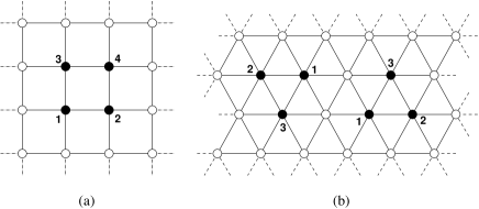
Figure 1: Examples of $0d$ profiles corresponding to maximal cavities for the first and second neighbor exclusion lattice gas in the square lattice (a) and the nearest neighbor exclusion lattice gas in the triangular lattice (b). The density can only have nonzero values at the black nodes (which define maximal cavities)).

If (4) were the final functional, evaluated at any maximal $0d$ profile (one corresponding to a maximal cavity) it should return the exact free energy. In the example, all maximal $0d$ profiles have the form illustrated in Fig. 1a. Let us now substitute this profile in (4) and see what comes out. For an easy way to do the evaluation, just imagine the graphs $\mathcal{C}_{k}(\mathbf{s})$ as windows which only allow to see the content of the lattice nodes they overlap. Then the sum over the lattice nodes implies that we must place these windows at every lattice site, evaluate the content and add up the results of these evaluations. When the density profile is a $0d$ one (as in Fig. 1a), all contributions will vanish except those for which the window overlaps at least one node of the $0d$ profile. In our example, this means that (4) will return

$$\begin{split}\beta\mathcal{F}^{\text{ex}}_{1}\left[\rho_{0d}\right]=&\,\Phi_{0}\left(\begin{picture}(22.0,10.0)(-6.0,2.0)\path(0,0)(10,0) \path(10,0)(10,10) \path(0,10)(10,10) \path(0,0)(0,10) \put(0.0,0.0){\circle*{4.0}} \put(-6.0,-4.0){{\tiny 1}} \put(10.0,0.0){\circle*{4.0}} \put(13.0,-4.0){{\tiny 2}} \put(0.0,10.0){\circle*{4.0}} \put(-6.0,10.0){{\tiny 3}} \put(10.0,10.0){\circle*{4.0}} \put(13.0,10.0){{\tiny 4}} \end{picture}\right)+\left[\Phi_{0}\left(\begin{picture}(21.0,6.0)(-2.0,-2.0)\path(4,0)(14,0) \put(4.0,0.0){\circle*{4.0}} \put(-2.0,-4.0){{\tiny 1}} \put(14.0,0.0){\circle*{4.0}} \put(16.0,-4.0){{\tiny 2}} \end{picture}\right)+\Phi_{0}\left(\begin{picture}(21.0,6.0)(-2.0,-2.0)\path(4,0)(14,0) \put(4.0,0.0){\circle*{4.0}} \put(-2.0,-4.0){{\tiny 3}} \put(14.0,0.0){\circle*{4.0}} \put(16.0,-4.0){{\tiny 4}} \end{picture}\right)\right]\\ &+\left[\Phi_{0}\left(\begin{picture}(10.0,10.0)(-4.0,3.0)\path(0,0)(0,10) \put(0.0,0.0){\circle*{4.0}} \put(3.0,-4.0){{\tiny 1}} \put(0.0,10.0){\circle*{4.0}} \put(3.0,10.0){{\tiny 3}} \end{picture}\right)+\Phi_{0}\left(\begin{picture}(10.0,10.0)(-4.0,3.0)\path(0,0)(0,10) \put(0.0,0.0){\circle*{4.0}} \put(3.0,-4.0){{\tiny 2}} \put(0.0,10.0){\circle*{4.0}} \put(3.0,10.0){{\tiny 4}} \end{picture}\right)\right]+\sum_{i=1}^{4}\Phi_{0}\left(\begin{picture}(10.0,6.0)(0.0,-2.0)\put(4.0,0.0){\circle*{4.0}} \put(7.0,-4.0){{\tiny$i$}} \end{picture}\right),\end{split}$$ (5)

where $\rho_{0d}(\mathbf{s})$ denotes a $0d$ profile of the form given in Fig. 1a. (Filled numbered circles in the diagrams represent actual evalutations of the density profile for the corresponding numbered nodes of the lattice.)

We can see that, apart from the exact value (the first term on the r.h.s.), there appear a number of spurious contributions. Therefore (4) cannot be the final functional. These spurious terms are like evaluations of $\rho_{0d}$ with non-maximal cavities, so we will try to eliminate them by adding new terms to (4) corresponding to non-maximal cavities, with the appropriate coefficients. Since a term like $\sum_{\mathbf{s}}\Phi_{0}(\begin{picture}(18.0,6.0)(0.0,-2.0)\path(4,0)(14,0) \put(4.0,0.0){\whiten\circle{4.0}} \put(14.0,0.0){\whiten\circle{4.0}} \end{picture})$ evaluated at $\rho_{0d}(\mathbf{s})$ will return $\Phi_{0}\left(\begin{picture}(21.0,6.0)(-2.0,-2.0)\path(4,0)(14,0) \put(4.0,0.0){\circle*{4.0}} \put(-2.0,-4.0){{\tiny 1}} \put(14.0,0.0){\circle*{4.0}} \put(16.0,-4.0){{\tiny 2}} \end{picture}\right)+\Phi_{0}\left(\begin{picture}(21.0,6.0)(-2.0,-2.0)\path(4,0)(14,0) \put(4.0,0.0){\circle*{4.0}} \put(-2.0,-4.0){{\tiny 3}} \put(14.0,0.0){\circle*{4.0}} \put(16.0,-4.0){{\tiny 4}} \end{picture}\right)+\sum_{i=1}^{4}\Phi_{0}\left(\begin{picture}(10.0,6.0)(0.0,-2.0)\put(4.0,0.0){\circle*{4.0}} \put(7.0,-4.0){{\tiny$i$}} \end{picture}\right)$, it seems reasonable to choose it to remove the first bracket on the r.h.s. of (5) (and the vertical one to remove the second bracket). Thus we use as our second ansatz

$$\beta\mathcal{F}^{\text{ex}}_{2}[\rho]=\sum_{\mathbf{s}\in\mathbb{Z}^{2}}\left[\Phi_{0}\left(\begin{picture}(18.0,10.0)(-4.0,2.0)\path(0,0)(10,0) \path(10,0)(10,10) \path(0,10)(10,10) \path(0,0)(0,10) \put(0.0,0.0){\whiten\circle{4.0}} \put(10.0,0.0){\whiten\circle{4.0}} \put(0.0,10.0){\whiten\circle{4.0}} \put(10.0,10.0){\whiten\circle{4.0}} \end{picture}\right)-\Phi_{0}\left(\begin{picture}(18.0,6.0)(0.0,-2.0)\path(4,0)(14,0) \put(4.0,0.0){\whiten\circle{4.0}} \put(14.0,0.0){\whiten\circle{4.0}} \end{picture}\right)-\Phi_{0}\left(\begin{picture}(8.0,10.0)(-4.0,3.0)\path(0,0)(0,10) \put(0.0,0.0){\whiten\circle{4.0}} \put(0.0,10.0){\whiten\circle{4.0}} \end{picture}\right)\right].$$ (6)

Note that in doing this, we have chosen new graphs $\mathcal{C}_{k}(\mathbf{s})$ and their corresponding coefficients $a_{k}$ in (1). When we insert $\rho_{0d}(\mathbf{s})$ in this new functional we obtain $\beta\mathcal{F}^{\text{ex}}_{2}[\rho_{0d}]=\Phi_{0}\left(\begin{picture}(22.0,10.0)(-6.0,2.0)\path(0,0)(10,0) \path(10,0)(10,10) \path(0,10)(10,10) \path(0,0)(0,10) \put(0.0,0.0){\circle*{4.0}} \put(-6.0,-4.0){{\tiny 1}} \put(10.0,0.0){\circle*{4.0}} \put(13.0,-4.0){{\tiny 2}} \put(0.0,10.0){\circle*{4.0}} \put(-6.0,10.0){{\tiny 3}} \put(10.0,10.0){\circle*{4.0}} \put(13.0,10.0){{\tiny 4}} \end{picture}\right)-\sum_{i=1}^{4}\Phi_{0}\left(\begin{picture}(10.0,6.0)(0.0,-2.0)\put(4.0,0.0){\circle*{4.0}} \put(7.0,-4.0){{\tiny$i$}} \end{picture}\right)$. We have indeed removed many spurious contributions, but there still remain some. It should now be clear that in order to remove the latter we must add to the previous ansatz the term $\sum_{\mathbf{s}\in\mathbb{Z}^{2}}\Phi_{0}(\begin{picture}(8.0,6.0)(0.0,-2.0)\put(4.0,0.0){\whiten\circle{4.0}} \end{picture})$. This way we obtain the functional (2), which was already derived in lafuente:2002a by a different procedure. It is straightforward to check that $\beta\mathcal{F}^{\text{ex}}[\rho_{0d}]=\Phi_{0}\left(\begin{picture}(22.0,10.0)(-6.0,2.0)\path(0,0)(10,0) \path(10,0)(10,10) \path(0,10)(10,10) \path(0,0)(0,10) \put(0.0,0.0){\circle*{4.0}} \put(-6.0,-4.0){{\tiny 1}} \put(10.0,0.0){\circle*{4.0}} \put(13.0,-4.0){{\tiny 2}} \put(0.0,10.0){\circle*{4.0}} \put(-6.0,10.0){{\tiny 3}} \put(10.0,10.0){\circle*{4.0}} \put(13.0,10.0){{\tiny 4}} \end{picture}\right)$, thus proving its exact dimensional crossover.

In order to be illustrative, let us apply this procedure again to obtain the FM functional for a different model: the nearest-neighbor exclusion lattice gas in the triangular lattice (hard hexagons). This example is different from the previous one in that it has two maximal cavities: and . Then, the first-step functional must be

$$\beta\mathcal{F}^{\text{ex}}_{1}[\rho]=\sum_{\mathbf{s}\in\mathbb{Z}^{2}}\left[\Phi_{0}\left(\begin{picture}(18.0,10.0)(-4.0,2.0)\path(0,0)(10,0)(5,8.7)(0,0) \put(0.0,0.0){\whiten\circle{4.0}} \put(10.0,0.0){\whiten\circle{4.0}} \put(5.0,8.7){\whiten\circle{4.0}} \end{picture}\right)+\Phi_{0}\left(\begin{picture}(18.0,10.0)(-4.0,2.0)\path(0,8.7)(10,8.7)(5,0)(0,8.7) \put(10.0,8.7){\whiten\circle{4.0}} \put(0.0,8.7){\whiten\circle{4.0}} \put(5.0,0.0){\whiten\circle{4.0}} \end{picture}\right)\right].$$ (7)

Corresponding to the existence of two different maximal cavities there are two different density profiles, as illustrated in Fig. 1b. The exact $0d$ dimensional crossover must be satisfied for both of them. Let us start by the one with a triangle-up shape and let us denote it $\rho_{0d}(\mathbf{s})$. Substituting it in each of the two terms of (7) we obtain (using again the window metaphor)

$$\begin{split}\sum_{\mathbf{s}\in\mathbb{Z}^{2}}\Phi_{0}\left(\begin{picture}(18.0,10.0)(-4.0,2.0)\path(0,0)(10,0)(5,8.7)(0,0) \put(0.0,0.0){\whiten\circle{4.0}} \put(10.0,0.0){\whiten\circle{4.0}} \put(5.0,8.7){\whiten\circle{4.0}} \end{picture}\right)=&\,\Phi_{0}\left(\begin{picture}(22.0,10.0)(-6.0,2.0)\path(0,0)(10,0)(5,8.7)(0,0) \put(0.0,0.0){\circle*{4.0}} \put(-6.0,-4.0){{\tiny 1}} \put(10.0,0.0){\circle*{4.0}} \put(12.0,-4.0){{\tiny 2}} \put(5.0,8.7){\circle*{4.0}} \put(8.0,8.0){{\tiny 3}} \end{picture}\right)+2\sum_{i=1}^{3}\Phi_{0}\left(\begin{picture}(10.0,6.0)(0.0,-2.0)\put(4.0,0.0){\circle*{4.0}} \put(7.0,-4.0){{\tiny$i$}} \end{picture}\right),\\ \sum_{\mathbf{s}\in\mathbb{Z}^{2}}\Phi_{0}\left(\begin{picture}(18.0,10.0)(-4.0,2.0)\path(0,8.7)(10,8.7)(5,0)(0,8.7) \put(10.0,8.7){\whiten\circle{4.0}} \put(0.0,8.7){\whiten\circle{4.0}} \put(5.0,0.0){\whiten\circle{4.0}} \end{picture}\right)=&\,\Phi_{0}\left(\begin{picture}(18.0,10.0)(-6.0,2.0)\path(0,0)(5,8.7) \put(0.0,0.0){\circle*{4.0}} \put(-6.0,-4.0){{\tiny 1}} \put(5.0,8.7){\circle*{4.0}} \put(8.0,8.0){{\tiny 3}} \end{picture}\right)+\Phi_{0}\left(\begin{picture}(18.0,10.0)(0.0,2.0)\path(10,0)(5,8.7) \put(10.0,0.0){\circle*{4.0}} \put(12.0,-4.0){{\tiny 2}} \put(5.0,8.7){\circle*{4.0}} \put(8.0,8.0){{\tiny 3}} \end{picture}\right)+\Phi_{0}\left(\begin{picture}(21.0,6.0)(-2.0,-2.0)\path(4,0)(14,0) \put(4.0,0.0){\circle*{4.0}} \put(-2.0,-4.0){{\tiny 1}} \put(14.0,0.0){\circle*{4.0}} \put(16.0,-4.0){{\tiny 2}} \end{picture}\right)\\ &+\sum_{i=1}^{3}\Phi_{0}\left(\begin{picture}(10.0,6.0)(0.0,-2.0)\put(4.0,0.0){\circle*{4.0}} \put(7.0,-4.0){{\tiny$i$}} \end{picture}\right).\end{split}$$ (8)

As in the previous example, to remove the “largest” spurious contributions (those of the dimers) we propose

$$\beta\mathcal{F}^{\text{ex}}_{2}[\rho]=\beta\mathcal{F}^{\text{ex}}_{1}[\rho]-\sum_{\mathbf{s}\in\mathbb{Z}^{2}}[\Phi_{0}\left(\begin{picture}(14.0,10.0)(-4.0,2.0)\path(0,0)(5,8.7) \put(0.0,0.0){\whiten\circle{4.0}} \put(5.0,8.7){\whiten\circle{4.0}} \end{picture}\right)+\Phi_{0}\left(\begin{picture}(14.0,10.0)(0.0,2.0)\path(10,0)(5,8.7) \put(10.0,0.0){\whiten\circle{4.0}} \put(5.0,8.7){\whiten\circle{4.0}} \end{picture}\right)+\Phi_{0}\left(\begin{picture}(18.0,6.0)(0.0,-2.0)\path(4,0)(14,0) \put(4.0,0.0){\whiten\circle{4.0}} \put(14.0,0.0){\whiten\circle{4.0}} \end{picture}\right)].$$ (9)

Substituting $\rho_{0d}(\mathbf{s})$ again we get $\beta\mathcal{F}^{\text{ex}}_{2}[\rho_{0d}]=\Phi_{0}\left(\begin{picture}(22.0,10.0)(-6.0,2.0)\path(0,0)(10,0)(5,8.7)(0,0) \put(0.0,0.0){\circle*{4.0}} \put(-6.0,-4.0){{\tiny 1}} \put(10.0,0.0){\circle*{4.0}} \put(12.0,-4.0){{\tiny 2}} \put(5.0,8.7){\circle*{4.0}} \put(8.0,8.0){{\tiny 3}} \end{picture}\right)-\sum_{i=1}^{3}\Phi_{0}\left(\begin{picture}(10.0,6.0)(0.0,-2.0)\put(4.0,0.0){\circle*{4.0}} \put(7.0,-4.0){{\tiny$i$}} \end{picture}\right)$, so we have to add a last correction for the point-like cavities, what finally leads to

$$\begin{split}\beta\mathcal{F}^{\text{ex}}[\rho]=&\,\sum_{\mathbf{s}\in\mathbb{Z}^{2}}[\Phi_{0}\left(\begin{picture}(18.0,10.0)(-4.0,2.0)\path(0,0)(10,0)(5,8.7)(0,0) \put(0.0,0.0){\whiten\circle{4.0}} \put(10.0,0.0){\whiten\circle{4.0}} \put(5.0,8.7){\whiten\circle{4.0}} \end{picture}\right)+\Phi_{0}\left(\begin{picture}(18.0,10.0)(-4.0,2.0)\path(0,8.7)(10,8.7)(5,0)(0,8.7) \put(10.0,8.7){\whiten\circle{4.0}} \put(0.0,8.7){\whiten\circle{4.0}} \put(5.0,0.0){\whiten\circle{4.0}} \end{picture}\right)-\Phi_{0}\left(\begin{picture}(14.0,10.0)(-4.0,2.0)\path(0,0)(5,8.7) \put(0.0,0.0){\whiten\circle{4.0}} \put(5.0,8.7){\whiten\circle{4.0}} \end{picture}\right)\\ &-\Phi_{0}\left(\begin{picture}(14.0,10.0)(0.0,2.0)\path(10,0)(5,8.7) \put(10.0,0.0){\whiten\circle{4.0}} \put(5.0,8.7){\whiten\circle{4.0}} \end{picture}\right)-\Phi_{0}\left(\begin{picture}(18.0,6.0)(0.0,-2.0)\path(4,0)(14,0) \put(4.0,0.0){\whiten\circle{4.0}} \put(14.0,0.0){\whiten\circle{4.0}} \end{picture}\right)+\Phi_{0}\left(\begin{picture}(8.0,6.0)(0.0,-2.0)\put(4.0,0.0){\whiten\circle{4.0}} \end{picture}\right)].\end{split}$$ (10)

This functional is exact for $\rho_{0d}(\mathbf{s})$. We would now have to check if the same occurs for the $0d$ cavity corresponding to the triangle-down in Fig. 1b, but symmetry considerations immediately show that this is the case. In general, checking dimensional crossover for a new $0d$ cavity may lead to the appearance of additional spurious contributions. These have to be eliminated by adding the corresponding terms to the functional.

Finally, notice that (10) coincides with the functional obtained in lafuente:2003p through a completely different (and far more involved) route.

Let us summarize the procedure to follow for an arbitrary lattice gas with hard-core interaction. The steps are:

(i) Determine the complete set of maximal $0d$ cavities of the model. If we denote them by $\mathcal{C}_{k}^{*}$ ($k=1,\ldots,m$), then the first-step approximation to the functional will be [$n^{(k)}(\mathbf{s})=\sum_{\mathbf{t}\in\mathcal{C}^{*}_{k}}\rho(\mathbf{t})$]

$$\beta\mathcal{F}^{\text{ex}}_{1}[\rho]=\sum_{\mathbf{s}\in\mathcal{L}}\sum_{k=1}^{m}\Phi_{0}\left(n^{(k)}(\mathbf{s})\right).$$ (11)

(ii) Select a maximal cavity $\mathcal{C}_{k}^{*}$ and let $\rho_{0d}(\mathbf{s})$ denote a generic density profile for it.

(iii) Insert $\rho_{0d}$ in the current functional, $\beta\mathcal{F}^{\text{ex}}_{i}[\rho]$, and see which spurious contributions appear. Identify the terms with the “largest” graphs (those not contained in any other of the graphs appearing, except $\mathcal{C}_{k}^{*}$) and pick one of them.

(iv) Construct the next step functional $\beta\mathcal{F}^{\text{ex}}_{i+1}[\rho]$ by adding to $\beta\mathcal{F}^{\text{ex}}_{i}[\rho]$ a new term, with its corresponding coefficient $a_{k}$, so that it eliminates the selected spurious contribution.

(v) Repeat steps (iii)–(v) until no spurious contribution remains. (Of course, one can exploit the symmetries of the model to resume several steps of this process in just one, as we have done in the examples.)

(vi) Repeat steps (ii)–(vi) until exhausting all maximal cavities.

The functional resulting from this process will be of the form (1) and will have, by construction, an exact $0d$ dimensional crossover. It can be proven that starting from (11) there is a unique functional of the form (1) with an exact $0d$ dimensional crossover, so any other procedure leading to it is equally valid. (In other words, the fact that we have chosen to remove the spurious terms in decreasing order of “size” is immaterial, but in doing so we abbreviate the process.) A sketch of the existence and uniqueness proof goes as follows (a more detailed account will be reported in lafuente:2004 ).

Let us form the set $\mathcal{P}$ with the lattice $\mathcal{L}$ and all maximal cavities $\mathcal{C}^{*}_{k}(\mathbf{s})$ ($\mathbf{s}\in\mathcal{L}$, $k=1,\dots,m$), and let us complete it with all nonempty intersection of any number of maximal cavities. For any $x,y\in\mathcal{P}$, we will say that $x\leq y$ iff all nodes of $x$ are in $y$. This transforms $\mathcal{P}$ into a partially ordered set or poset. Any interval $[x,y]\equiv\{z\in\mathcal{P}\,:\,x\leq z\leq y\}$ is a finite subset of $\mathcal{P}$, so $\mathcal{P}$ is a locally finite poset. Locally finite posets have the property stanley:1999 that for any mapping $f:\mathcal{P}\mapsto V$, with $V$ a vector space, there exists $g:\mathcal{P}\mapsto V$ such that

$$f(x)=\sum_{y\leq x}g(y),\qquad g(x)=\sum_{y\leq x}f(y)\mu(y,x).$$ (12)

The way to prove this is by inserting the second expression into the first, what leads to

$$\mu(x,x)=1,\qquad\mu(y,x)=-\sum_{y<z\leq x}\mu(z,x),$$ (13)

a recursion which defines the (integer) coefficients $\mu(y,x)$. This scheme is referred to in the literature as a Möbius inversion, and $\mu(y,x)$ is a Möbius function stanley:1999 .

For the poset $\mathcal{P}$ defined above, let $\mathcal{V}$ be the space of density functionals and take $f(x)\equiv\mathcal{F}_{x}^{\rm ex}[\rho]$ the (exact) excess free energy functional of a given model on the graph $x$. Specializing (12) to $x=\mathcal{L}$,

$$\mathcal{F}_{\mathcal{L}}^{\rm ex}[\rho]=\Psi_{\mathcal{L}}[\rho]+\sum_{x<\mathcal{L}}\big{[}-\mu(x,\mathcal{L})\big{]}\mathcal{F}_{x}^{\rm ex}[\rho].$$ (14)

where $\Psi_{\mathcal{L}}[\rho]$ is an unknown functional. The sum on the r.h.s. of (14) only contains evaluations of $\mathcal{F}_{x}^{\rm ex}[\rho]$ for $0d$ cavities and so is an expression similar to (1). Now let $\rho^{0d}_{x}(\mathbf{s})$ a generic $0d$ density profile for cavity $x$. Then,

$$\mathcal{F}_{y}^{\rm ex}[\rho^{0d}_{x}]=\begin{cases}0&\mbox{if $x\cap y=\emptyset$,}\\ \mathcal{F}_{y\cap x}^{\rm ex}[\rho]&\mbox{otherwise.}\end{cases}$$ (15)

As $x\cap\mathcal{L}=x$, evaluating (14) for $\rho^{0d}_{x}(\mathbf{s})$ yields

$$\Psi_{\mathcal{L}}[\rho^{0d}_{x}]=\sum_{z\leq x}\nu(z,x)\mathcal{F}_{z}^{\rm ex}[\rho],\quad\nu(z,x)=\sum_{y\cap x=z}\mu(y,\mathcal{L}),$$ (16)

and it is a consequence of Weisner’s theorem stanley:1999 that $\nu(z,x)=0$ for any $x<\mathcal{L}$; therefore $\Psi_{\mathcal{L}}[\rho^{0d}_{x}]=0$ or, in other words, the sum on the r.h.s. of (14) is exact for any $0d$ cavity.

This completes the proof that the requirement of an exact dimensional reduction to $0d$ cavities leads to a functional of the form (1). As to the uniqueness, it suffices to realize that $\nu(z,x)=0$ (a necessary condition for a functional of the form (1) to have an exact dimensional reduction to $0d$ cavities) is a particular case of the recurrence (13), whose only solution is $\mu(x,\mathcal{L})$.

With this method one can easily recover all functionals previously obtained in Refs. lafuente:2002a ; lafuente:2003b ; lafuente:2003p and obtain those of virtually any other hard-core lattice gas t-model . One further striking feature of all functionals obtained in this way is that they also have an exact dimensional crossover to one dimension, simply because the exact one-dimensional functional is of the form (1) lafuente:2002a ; lafuente:2003p .

Clearly the procedure presented above has no restriction in its application other than the determination of the maximal cavities. It can be applied to particles of any shape, in any lattice (including regular lattices, Bethe lattices, Husimi trees, etc.) and in any dimension. It can even be applied to mixtures, either additive or non-additive, provided a $0d$ cavity is properly defined as a superposition of cavities, one for each species, such that at most one particle of only one species can be placed in it (see lafuente:2002a for more details).

The readers familiar with Kikuchi’s cluster variation method may have recognized a similarity with the procedure we have presented here. The connection is more prominent through the Möbius inversion formula morita and will be properly discussed elsewhere lafuente:2004 .

Finally, the theory can be generalized in several ways. First of all, we have already mentioned that there is a straightforward extension to mixtures which recovers the functionals for mixtures already derived in lafuente:2002a ; lafuente:2003b ; lafuente:2002b . A second extension is the inclusion of “extended” $0d$ cavities in which there can be up to $n$ particles. We have already checked that the inclusion of two-particle $0d$ cavities for the Ising lattice gas (which has repulsive and attractive interactions!) yields the functional obtained from the cluster variation method at the level of the Bethe approximation ising , which is exact in one dimension. Finally, there is a third extension for lattice gases in the presence of a porous matrix that we have already began to explore schmidt:2003 . Work along these lines is in progress.

References

• (1) M. Nieswand, W. Dieterich and A. Majhofer, Phys. Rev. E47, 718 (1993); M. Nieswand, A. Majhofer and W. Dieterich, Phys. Rev. E48, 2521 (1993); D. Reinel, W. Dieterich and A. Majhofer, Phys. Rev. E50, 4744 (1994).
• (2) S. Prestipino and P. V. Giaquinta, J. Phys.: Condens. Matter 15, 3931 (2003); S. Prestipino, J. Phys.: Condens. Matter 15, 8065 (2003).
• (3) J. Reinhard, W. Dieterich, P. Maass and H. L. Frisch, Phys. Rev. E61, 422 (2000).
• (4) L. Lafuente and J. A. Cuesta, J. Phys.: Condens. Matter 14, 12079 (2002).
• (5) J. A. Cuesta and Y. Martínez-Ratón, Phys. Rev. Lett. 78, 3681 (1997).
• (6) L. Lafuente and J. A. Cuesta, Phys. Rev. E68, 066120 (2003).
• (7) G. Biroli and M. Mézard, Phys. Rev. Lett. 88, 025501 (2002).
• (8) E. Kierlik, P. A. Monson, M. L. Rosinberg, L. Sarkisov and G. Tarjus, Phys. Rev. Lett. 87, 055701 (2001).
• (9) S. T. Chui and J. D. Weeks, Phys. Rev. B23, 2438 (1981).
• (10) M. Ya. Azbel, Phys. Rev. A20, 1671 (1979).
• (11) Y. Rosenfeld, M. Schmidt, H. Löwen and P. Tarazona, J. Phys.: Condens. Matter 8, L577 (1996); P. Tarazona and Y. Rosenfeld, Phys. Rev. E55, R4873 (1997); P. Tarazona, Phys. Rev. Lett. 84, 694 (2000).
• (12) L. Lafuente and J. A. Cuesta, Phys. Rev. Lett. 89, 145701 (2003).
• (13) L. Lafuente and J. A. Cuesta, J. Chem. Phys. 119, 10832 (2003).
• (14) L. Lafuente and J. A. Cuesta, to be published (2004).
• (15) Applying this procedure, it should now be straightforward to obtain, e.g., the FM functional for the first and second neighbor exclusion lattice gas in the triangular lattice (the so-called t-model of ref. prestipino:2003 ) as βex[ρ]=𝐬2[Φ0(0,0)10,0)(5,8.7)(0,0) 5,8.7)15,8.7)(10,0) \whiten\whiten\whiten\whiten)+Φ0(0,0)10,0)(5,8.7)(0,0) 5,8.7)-5,8.7)(0,0) \whiten\whiten\whiten\whiten)+Φ0(0,0.7)10,0.7)(5,-8)(0,0.7) 0,0.7)5,9.4)(10,0.7) \whiten\whiten\whiten\whiten)2Φ0(0,0)10,0)(5,8.7)(0,0) \whiten\whiten\whiten)2Φ0(0,8.7)10,8.7)(5,0)(0,8.7) \whiten\whiten\whiten)+Φ0(\whiten)]𝛽subscriptexdelimited-[]𝜌subscript𝐬superscript2delimited-[]subscriptΦ00,0)10,0)(5,8.7)(0,0) 5,8.7)15,8.7)(10,0) \whiten\whiten\whiten\whitensubscriptΦ00,0)10,0)(5,8.7)(0,0) 5,8.7)-5,8.7)(0,0) \whiten\whiten\whiten\whitensubscriptΦ00,0.7)10,0.7)(5,-8)(0,0.7) 0,0.7)5,9.4)(10,0.7) \whiten\whiten\whiten\whiten2subscriptΦ00,0)10,0)(5,8.7)(0,0) \whiten\whiten\whiten2subscriptΦ00,8.7)10,8.7)(5,0)(0,8.7) \whiten\whiten\whitensubscriptΦ0\whiten\beta\mathcal{F}_{\mathrm{ex}}[\rho]=\sum_{\mathbf{s}\in\mathbb{Z}^{2}}\big{[}\Phi_{0}\left(\begin{picture}(23.0,10.0)(-4.0,2.0)\path(0,0)(10,0)(5,8.7)(0,0) \path(5,8.7)(15,8.7)(10,0) \put(0.0,0.0){\whiten\circle{4.0}} \put(10.0,0.0){\whiten\circle{4.0}} \put(5.0,8.7){\whiten\circle{4.0}} \put(15.0,8.7){\whiten\circle{4.0}} \end{picture}\right)+\Phi_{0}\left(\begin{picture}(22.0,10.0)(-9.0,2.0)\path(0,0)(10,0)(5,8.7)(0,0) \path(5,8.7)(-5,8.7)(0,0) \put(0.0,0.0){\whiten\circle{4.0}} \put(10.0,0.0){\whiten\circle{4.0}} \put(5.0,8.7){\whiten\circle{4.0}} \put(-5.0,8.7){\whiten\circle{4.0}} \end{picture}\right)+\Phi_{0}\left(\begin{picture}(18.0,14.0)(-4.0,-4.0)\path(0,0.7)(10,0.7)(5,-8)(0,0.7) \path(0,0.7)(5,9.4)(10,0.7) \put(10.0,0.7){\whiten\circle{4.0}} \put(0.0,0.7){\whiten\circle{4.0}} \put(5.0,-8.0){\whiten\circle{4.0}} \put(5.0,9.4){\whiten\circle{4.0}} \end{picture}\right)-2\Phi_{0}\left(\begin{picture}(18.0,10.0)(-4.0,2.0)\path(0,0)(10,0)(5,8.7)(0,0) \put(0.0,0.0){\whiten\circle{4.0}} \put(10.0,0.0){\whiten\circle{4.0}} \put(5.0,8.7){\whiten\circle{4.0}} \end{picture}\right)-2\Phi_{0}\left(\begin{picture}(18.0,10.0)(-4.0,2.0)\path(0,8.7)(10,8.7)(5,0)(0,8.7) \put(10.0,8.7){\whiten\circle{4.0}} \put(0.0,8.7){\whiten\circle{4.0}} \put(5.0,0.0){\whiten\circle{4.0}} \end{picture}\right)+\Phi_{0}\left(\begin{picture}(8.0,6.0)(0.0,-2.0)\put(4.0,0.0){\whiten\circle{4.0}} \end{picture}\right)\big{]} (the meaning of the diagrams should be self-evident).
• (16) T. Morita, J. Stat. Phys. 59, 819 (1990); Prog. Theor. Phys. 115, 27 (1994).
• (17) R. P. Stanley, Enumerative combinatorics, vol. 1 (Cambridge University Press, Cambridge, 1999), pp. 116–124.
• (18) M. Schmidt, L. Lafuente and J. A. Cuesta,J. Phys.: Condens. Matter 15, 4695 (2003).
• (19) D. R. Bowman and K. Levin, Phys. Rev. B25, 3438 (1982).