Double-Layer Bose-Einstein Condensates with Large Number of Vortices

Abstract

In this paper we systematically study the double layer vortex lattice model, which is proposed to illustrate the interplay between the physics of a fast rotating Bose-Einstein condensate and the macroscopic quantum tunnelling. The phase diagram of the system is obtained. We find that under certain conditions the system will exhibit one novel phase transition, which is consequence of competition between inter-layer coherent hopping and inter-layer density-density interaction. In one phase the vortices in one layer coincide with those in the other layer. And in another phase two sets of vortex lattices are staggered, and as a result the quantum tunnelling between two layers is suppressed. To obtain the phase diagram we use two kinds of mean field theories which are quantum Hall mean field and Thomas-Fermi mean field. Two different criteria for the transition taking place are obtained respectively, which reveals some fundamental differences between these two mean field states. The sliding mode excitation is also discussed.

I Introduction

In the recent years remarkable progress has been made in the field of ultracold quantum gas, among which the achievement of fast rotating boson gases and the realization of Mott insulator to superfluid transition are two important ones. The physics of these two phenomena have attracted a lot of theoretical and experimental interests.

It has been long predicted that there exists a quantum phase transition from the superfluid phase to the Mott insulator phase in the boson Hubbard model as the hopping parameter decreases, and recently it has been observed in ultracold Bose atoms in the optical lattice.Bloch The Mott insulator phase is characterized by the loss of phase coherence among the sites and the whole system becoming fragmented. The essential physics of this transition can be demonstrated by a simpler model, namely the bosons confined in a double well potential. In the strong tunnelling limit, the condensates located in the two wells develop a relative phase and the ground state is described by a coherent state. In the opposite limit, the relative number fluctuation is suppressed and each condensate has determined atom number.Legget The ground state is well described by a Fock state. Hence there exists a crossover from the coherent regime to the Fock regime as the parameter $t/U$ decreasing in the two-well system.

On the other hand, the boson atoms confined in the a quasi-two-dimensional harmonic trap can now be rotated fast enough that the rotation frequency is very close to trapping frequency.ketterle2 cornell It has been observed that such rapid rotating condensate contains a large number of vortices and they form a regular triangular lattice. The fast rotating BEC is also characterized by two regimes. One is called the Thomas-Fermi mean field (TFMF) regime, where the interaction energy dominates over the kinetic energy. The other is the quantum Hall mean field (QHMF) regime, in which the energy gap between single particle Landau levels is much larger than the interaction energy.Ho Based on the quantum Hall mean field theory the two-component fast rotating BEC was firstly studied by Mueller and Ho.Mueller The relative displacement $r_{0}$ between the two sets of vortex lattices was found to be a non-vanishing value for even a little positive inter-special interaction $U_{12}$. With the increase of $U_{12}$ the vortex lattice will experience a structure transition from triangular to square.Mueller Similar conclusions was later obtained by numerical study in the Thomas-Fermi regime.ueda All these have motivated us to present a novel model that contains the above two physical features and illustrates their interplay.

II The Model

In this section we introduce our model for double-layer rotating BEC. The BEC is confined in a harmonic trap in the $xy$ plane and high angular momentum with respect to $z$ direction is imparted into the condensate. Along the $z$ direction the condensate is confined in a double well potential. Thus two sets of vortex lattices are formed in the wells and they couple to each other via quantum tunnelling through the barrier between the wells. We call such a system double-layer vortex lattice and schematically illustrate it in Fig.1. It is believed to be experimentally realizable due to the recent technique progress on double well potentialKetterledwell Kiltzing . The conclusions drawn from this model can be directly generalized to the case that a fast rotating BEC is cut into pieces by applying an optical lattice along the $z$-direction as shown in Fig.1.

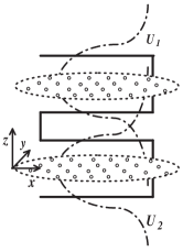
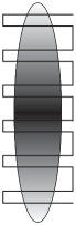
Figure 1: Left: The double-layer vortex lattice system;   Right: The rotating BEC confined in a optical lattice in the $z$-direction.

When these two layers are well separated by a high potential barrier, the wave function overlapping along the $z$-direction is sufficiently small, the phase fluctuation between the wells is strong enough that the inter-layer phase coherence is lost and the coherent hopping is suppressed. This regime is called Fock regime because the particle number in each well is almost fixed. From the work of Mueller and Ho Mueller we know that in this regime the relative displacement $r_{0}$ will take a non-zero value due to the inter-layer density-density interaction. However this effect may be frangible because this interaction is very weak in this case.

While in the coherent regime the whole system is described by a macroscopic wave function

$$\Psi=\sqrt{2}\left[\sqrt{n_{1}}u_{1}(z)\varphi_{1}(x,y)+\sqrt{n_{2}}e^{i\theta}u_{2}(z)\varphi_{2}(x,y)\right)]$$ (1)

and the energy functional in the rotating frame is written as

$$H=\int dxdydz\left[\Psi^{*}(h_{z}+h_{x,y}-\mu)\Psi+\frac{2\pi\hbar^{2}a_{sc}N}{m}|\Psi|^{4}\right],$$ (2)

where

$$h_{z}=-\frac{\hbar^{2}}{2m}\frac{d^{2}}{dz^{2}}+V_{\text{dou}}.$$ (3)

Here $V_{\text{dou}}$ is the double well potential. $u_{1,2}=(u_{s}\pm u_{a})/2$ represent the wave packets localized in each well. Here $u_{s}$ and $u_{a}$ are the normalized ground state and the first excited state of $h_{z}$, whose eigenvalues are assumed to be far below other eigenvalues. $u_{s}$ and $u_{a}$ are symmetric and antisymmetric respectively, the energy splitting between them is denoted by $t$.

In the rotating frame, the single particle Hamiltonian in $xy$ plane, $h_{x,y}$, is

$$h_{x,y}=-\frac{\hbar^{2}}{2m}\nabla^{2}+\frac{1}{2}m\omega_{\perp}^{2}r^{2}-\Omega L_{z}$$ (4)

where $\omega_{\perp}$ is the trapping frequency and $\Omega$ is the rotation frequency. In the fast rotating condensate, $\Omega$ is quite close to $\omega_{\perp}$ and the condensate in each well forms a vortex lattice, denoted by $\varphi_{1}$ and $\varphi_{2}$ respectively. We define $\Delta N=(n_{1}-n_{2})N$ as the relative atom number difference between the two condensates, and $\theta$ is the relative phase. Corresponding to a normalized $\Psi$, $n_{1}+n_{2}$ should be equal to unity.

Substituting the order parameter(1) into the energy functional(2), the energy functional can be written as follows:approximation

$$E = -t\sqrt{n_{1}n_{2}}\left(\cos\theta\Re\int dxdy\varphi_{1}^{*}\varphi_{2}+\sin\theta\Im\int dxdy\varphi_{1}^{*}\varphi_{2}\right)+\int dxdy\left[n_{1}\varphi_{1}^{*}h_{xy}\varphi_{1}+n_{2}\varphi_{2}^{*}h_{xy}\varphi_{2}\right]$$ (5)

$$+ 4U\left(n_{1}^{2}\int dxdy|\varphi_{1}|^{4}+n_{2}^{2}\int dxdy|\varphi_{2}|^{4}\right)$$

$$+ 8U_{12}n_{1}n_{2}\left(2\int dxdy|\varphi_{1}|^{2}|\varphi_{2}|^{2}+\cos 2\theta\Re\int dxdy(\varphi_{1}^{*}\varphi_{2})^{2}-\sin 2\theta\Im\int dxdy(\varphi_{1}^{*}\varphi_{2})^{2}\right).$$

$\Re$ and $\Im$ stand for the real part and imaginary part respectively. Here we denote $U=2\pi\hbar^{2}a_{sc}N(\int dzu_{1,2}^{4})/m$ and $U_{12}=2\pi\hbar^{2}a_{sc}N(\int dzu_{1}^{2}u_{2}^{2})/m$. In this case $U$ is always larger than $U_{12}$ by at least one order of magnitude, so the energy minimum occurs at $n_{1}=n_{2}$ and the two layers have the same lattice type.

The main goal of this paper is to perform a systematic study of the double-layer vortex lattice system based on the energy functional(5), including the mean field phase diagram, phase transition and excitations. Several key points will be contained. Let us first briefly introduce them in the following.

As shown in the case of two-component rotating BECMueller ueda , the repulsive density-density interaction term $|\varphi_{1}|^{2}|\varphi_{2}|^{2}$ favors a situation in which the high density region of one condensate coincides with the low density region of the other, therefore the vortices of the two condensates should avoid each other. The difference between the current model and the two-component case is the presence of coherent hopping terms such as $\varphi_{1}^{*}\varphi_{2}$ and $\varphi_{1}^{*2}\varphi_{2}^{2}$, which favor the vortices in two layers being coincident. Hence the double-layer model is of interest because there exist competing terms in the energy functional, and it is natural to ask whether and how this competition will manifest itself in a quantum phase transition.

We find out in this paper that such a transition does not always take place, and we will answer the question under which condition the competition will result in a phase transition. Because a qualitative investigation of the inter-layer physics directly relies on how we describe the vortex lattice state, and we know that there exist two different mean field regimes for the fast rotating BEC called Thomas-Fermi regime and quantum Hall regimes, which are distinguished by the radio of the kinetic energy to the interaction energy, we study the issue with two kinds of mean field theories respectively and obtain two different criteria for the inter-layer transition taking place in these two regimes. We will remark in the end of this paper that the difference reveals some intrinsic properties of these two mean field ansatzs.

The model studied here is also different from the double well model because the condensate in each well has a vortex lattice structure of its own, which is beyond the single model approximation used in the discussion of double-well BEC. It is known that the transition from coherent regime to Fock regime is driven by the hopping element between two condensates. Here we will find that the hopping element, as well as relative phase fluctuation, is not only dependent on the wave function overlapping along the $z$-direction as in the double well case, but also depend on the integral $\int dxdy\varphi_{1}^{*}\varphi_{2}$. Therefore, when two sets of vortex lattices do not coincide with each other, the integral will be relatively small and the tunnelling between two layers will be suppressed. This presents a new mechanism for the transition from coherent regime to Fock regime, which is another key point discussed in this paper.

For the case that the transition can occur, we analytically give the phase boundary between the coincident lattice phase and the staggered lattice phase. For the case that the transition is absent, we find that the relative phase $\theta$ between two condensates will experience a second order change as $t/U_{12}$ decreases. After investigating a new excitation mode called vortex lattice’s sliding mode, we point out that such a change will manifest itself in the frequency of sliding mode.

The paper is organized as follows. In the following section, we will first study the case that the vortex lattice state is in the QHMF regime. After a brief review of QHMF theory in the first subsection III.1, we focus on the transition for triangular vortex lattice in the subsection III.2, and we discuss the sliding mode in the subsection III.3. Then in the next subsection III.4 we will generalize our discussion to arbitrary lattice type and summarize the conclusions in the subsection III.5. In the section IV, we focus on TFMF regime and present a wave function ansatz to describe vortex lattice state with the help of Thomas-Fermi approximation. Using this ansatz we will revisit the issue studied in the third section. The results obtained from the two different mean field theories are compared. We remark in the last section that these difference distinguish the intrinsic properties of the two regimes.

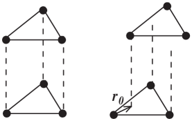
Figure 2: Left: The coincident lattice phase. Right: The staggered lattice phase. The main part of this paper are concerned with under which condition the transition between these two phases can take place and determining the phase boundary.

III Quantum Hall Mean Field Regime

III.1 Review of QHMF Theory

Here we first briefly review the quantum Hall mean field theory for single rotating condensate. We notice that $h_{x,y}$ can be rewritten as

$$h_{x,y}=\frac{1}{2m}\left(-i\hbar\nabla-m\omega_{\perp}\hat{z}\times\vec{r}\right)^{2}+\hbar(\omega_{\perp}-\Omega)L_{z}\ \ .$$ (6)

The Hamiltonian is identical to that describing a two-dimensional particle moving in a perpendicular magnetic field in the symmetric gauge. The eigenstates of $h_{x,y}$ are the Landau levels. Defining the complex variable $w=(x+iy)/2a_{\perp}$ and $w^{*}=(x-iy)/2a_{\perp}$ with $a_{\perp}=\sqrt{{\hbar}/{m\omega_{\perp}}}$, in the quantum Hall mean field picture the system is forced into the lowest Landau level (LLL) under the condition that $\Omega$ is close to $\omega_{\perp}$ and $\hbar\Omega$ is much larger than the interaction energy, and consequently the macroscopic wave function $\varphi_{1,2}(x,y)$ are analytical functions of the complex variable $w$ apart from a Gaussian factor. In the LLL, the first term in Eq.(6) gives the same expectation value for all states and can be neglected from the energy functional. The expectation value of the single particle Hamiltonian turns out to beHo

$$\langle h_{x,y}\rangle=\hbar(\omega_{\perp}-\Omega)\langle|w|^{2}\rangle.$$ (7)

It is noticed that for the vortex lattice states all first order zeros of the entire functions $\varphi$, which are the locations of vortices, form a regular lattice. Besides, the condensate density should be circular symmetric if the confinement potential is isotropic. These two requirements uniquely determine that $\varphi$ should be in the following form:

$$\varphi_{\text{qh}}=\theta(\zeta,\tau)\exp\left(\frac{\pi w^{2}}{2v_{c}}\right)\exp\left(-\frac{r^{2}}{2a_{\perp}^{2}}\right).$$ (8)

Here $\theta(\zeta,\tau)$ is the Jacobi theta function. We denote $b_{1}$ and $b_{2}$ as the basis vectors of the lattice, $\tau=b_{2}/b_{1}=u+iv$ characterizes the lattice type and $v_{c}=b_{1}^{2}v$ is the area of a unit cell. The argument $\zeta$ of the theta function is defined by scaling $\omega$ with $b_{1}$, i.e. $\zeta=w/b_{1}$. The explicit form of $\theta(\zeta,\tau)$ is

$$\theta(\zeta,\tau)=\frac{1}{i}\sum\limits_{n=-\infty}^{+\infty}(-1)^{n}e^{i\pi\tau(n+\frac{1}{2})^{2}+2\pi i\zeta(n+\frac{1}{2})}.$$ (9)

In Ref.Mueller it has been shown that from Eq.(9) one can obtain that

$$|\varphi|^{2}=\frac{1}{\pi\sigma^{2}}\sum\limits_{\vec{K}}g_{K}\exp(i\vec{K}\cdot\vec{r})\exp(-r^{2}/\sigma^{2}),$$ (10)

where $\vec{K}_{m_{1}m_{2}}=m_{1}\vec{K}_{1}+m_{2}\vec{K_{2}}$ are the reciprocal lattice vectors,

$$g_{K}=(-1)^{m_{1}+m_{2}+m_{1}m_{2}}e^{-v_{c}|K|^{2}/8\pi}\sqrt{v_{c}/2}$$ (11)

and

$$v_{c}|K|^{2}=(2\pi)^{2}v^{-1}[(vm_{1})^{2}+(m_{2}+um_{1})^{2}].$$ (12)

The condensate radius $\langle r^{2}\rangle$ is modified to $\sigma^{2}$ by the presence of large number of vortices, and

$$\sigma^{-2}=a_{\perp}^{-2}-\pi v_{c}^{-1}.$$ (13)

Furthermore, with the help of Eq.(10) we can evaluate the self-interaction energy of each condensate

$$\int dxdy|\varphi|^{4}=\frac{1}{2\pi\sigma^{2}}\frac{\sum\limits_{K,K^{\prime}}g_{K}g_{K^{\prime}}e^{-\sigma^{2}|K+K^{\prime}|^{2}/2}}{\left(\sum\limits_{K}g_{K}e^{-\sigma^{2}{K}^{2}/4}\right)^{2}}.$$ (14)

In the larger vortex number limit, $\pi\sigma^{2}/v_{c}\gg 1$, we only keep the $K=-K^{\prime}$ terms in the numerator and $K=0$ term in the denominator. The integral(14) can then be simplified to

$$\int dxdy|\varphi|^{4}=\frac{1}{2\pi\sigma^{2}}\sum\limits_{K}\left|\frac{g_{K}}{g_{0}}\right|^{2}=\frac{I_{1}}{2\pi\sigma^{2}}.$$ (15)

Then we can minimize the energy functional, including Eq.(7) and Eq.(15), to obtain the average vortex density and the vortex lattice structure. We notice that all the information about the lattice type is contained in $I_{1}$. Minimizing $I_{1}$ we will find the lattice structure being triangular. However, if some additional factors are included, such as the anisotropy of the confinement potential, it is also possible for the lattice structure changing from triangular to others.stript StriptEx MOktel

III.2 Double-Layer Triangular Vortex Lattice

Now we begin to discuss two coupled rotating BECs by using QHMF theory. The inter-layer interaction and the coherent hopping between two condensates should be considered. Because in this model $U_{12}\ll U$ and the hopping terms are almost independent of the lattice structure as we will show later, we can assume that the inter-layer coupling will not change the lattice structure of each condensate. In this subsection we will firstly focus on the triangular lattice.

It has been found in Ref.Mueller that

$$\int dxdy|\varphi_{1}|^{2}|\varphi_{2}|^{2}=\frac{1}{2\pi\sigma^{2}}\sum\limits_{K}\left|\frac{g_{K}}{g_{0}}\right|^{2}\cos\vec{K}\cdot\vec{r}_{0}.$$ (16)

Because $g_{K}$ exponentially depend on $|K|$ as one can see from Eq.(11), only several terms such as $g_{00}$, $g_{0,\pm 1}$, $g_{\pm,0}$ and $g_{\pm 1,\pm 1}$ need to be considered. For triangular lattice we have $I_{1}=1.1596$, and

$$\int dxdy|\varphi_{1}|^{2}|\varphi_{2}|^{2}=\frac{1}{2\pi\sigma^{2}}[1+f(\vec{r}_{0})],$$ (17)

where

$$f(\vec{r_{0}})=C\sum\limits_{K_{01},K_{10},K_{1-1}}\cos\vec{K}\cdot\vec{r}_{0}$$ (18)

with $C=0.0532$. The minimum value of $f(r_{0})$ is $-3C/2$ which occurs at $r_{0}=(b_{1}+b_{2})/3$, and its maximum is $3C$ occurring at $r_{0}=0$.

Using Eq.(9) we evaluate the coherence terms (for details see the appendix A). Considering the number of vortices contained in the cloud $N_{v}=\pi\sigma^{2}/v_{c}\gg 1$ and following the same approximation made in Ref.Mueller , we drop all the $K\neq 0$ terms and obtain the simplified expression of Eq.(69) is

$$\Re\int dxdy\varphi^{*}_{1}\varphi_{2}=\exp\left(-N_{v}\frac{\pi}{v_{c}}r_{0}^{2}\right)$$ (19)

and

$$\Im\int dxdy\varphi^{*}_{1}\varphi_{2}=0.$$ (20)

Similarly we obtain the real part of the two-particle coherent hopping term as

$$\Re\int dxdy(\varphi_{1}^{*}\varphi_{2})^{2} = \frac{1}{2\pi\sigma^{2}}\sum\limits_{K}\left|\frac{g_{K}}{g_{0}}\right|^{2}\exp\left(-N_{v}\frac{\pi}{2v_{c}}r_{0}^{2}\right)$$ (21)

$$= \frac{I_{1}}{2\pi\sigma^{2}}\exp\left(-N_{v}\frac{\pi}{2v_{c}}r_{0}^{2}\right)$$

while its imaginary part vanishes. These coherent terms are exponentially dependent on the relative displacement $r_{0}$, and the exponential factor $N_{v}$ is very large for the case discussed in this paper. This indicates that the coherent terms will be exponentially small and the phase fluctuation will be enhanced when $r_{0}^{2}$ is comparable to $v_{c}$. It means that if the competition results in a transition from $\vec{r}_{0}=0$ to a non-vanishing $\vec{r}_{0}$, such a transition will be accompanied by the loss of phase coherence.

According to above discussions, the energy functional can be rewritten as following:

$$E=-\frac{t}{2}\cos\theta\exp\left(-N_{v}\frac{\pi}{v_{c}}r_{0}^{2}\right)+\hbar(\omega-\Omega)\frac{\sigma^{2}}{a_{\perp}^{2}}$$

$$+\frac{1}{2\pi\sigma^{2}}[2UI+4U_{12}+4U_{12}f(r_{0})$$

$$+2U_{12}I\cos 2\theta\exp\left(-N_{v}\frac{\pi}{2v_{c}}r_{0}^{2}\right)].$$

(22)

In the following we will minimize the energy functional to obtain the mean field ground state, and then discuss the phase diagram. First of all we minimize $E$ with respect to $\sigma$. As $U_{12}/U$ is a small parameter, we can expand the result to its first order, which yields that

$$E=-\frac{t}{2}\cos\theta e^{-N_{v}\frac{\pi r_{0}^{2}}{v_{c}}}+\frac{AU_{12}}{\sqrt{I_{1}}U}\left[f(r_{0})+\frac{I_{1}}{2}\cos 2\theta e^{-N_{v}\frac{\pi r_{0}^{2}}{2v_{c}}}\right].$$ (23)

Here $A$ is defined as $\sqrt{U(\omega_{\perp}-\Omega)/(\pi a_{\perp}^{2})}$. Two constant terms, $2A\sqrt{I_{1}}$ and $AU_{12}/(\sqrt{I_{1}}U)$ have been neglected in the above expression.

When $t>4A\sqrt{I_{1}}U_{12}e^{-N_{v}\frac{\pi r_{0}^{2}}{2v_{c}}}/U$, the expectation value of the relative phase $\bar{\theta}$ tends to be zero, and then

$$E=-\frac{t}{2}\left(e^{-N_{v}\frac{\pi r_{0}^{2}}{2v_{c}}}-\frac{AU_{12}\sqrt{I_{1}}}{2Ut}\right)^{2}+\frac{A^{2}U_{12}^{2}I_{1}}{8U^{2}t}+\frac{AU_{12}}{\sqrt{I_{1}}U}f(r_{0}).$$ (24)

While when $t<4A\sqrt{I_{1}}U_{12}e^{-N_{v}\frac{\pi r_{0}^{2}}{2v_{c}}}/U$, $\bar{\theta}$ will gradually change from zero to $\pi/2$ with $t$ decreasing, and

$$\cos\bar{\theta}=\frac{tU}{4\sqrt{I_{1}}AU_{12}}\exp\left(-N_{v}\frac{\pi}{2v_{c}}r_{0}^{2}\right),$$ (25)

the energy minimum will be

$$E=-\frac{t^{2}Ue^{-N_{v}\frac{3\pi r_{0}^{2}}{2v_{c}}}}{16AU_{12}\sqrt{I_{1}}}-\frac{AU_{12}\sqrt{I_{1}}}{2U}e^{-N_{v}\frac{\pi r_{0}^{2}}{2v_{c}}}+\frac{AU_{12}}{\sqrt{I_{1}}U}f(r_{0}).$$ (26)

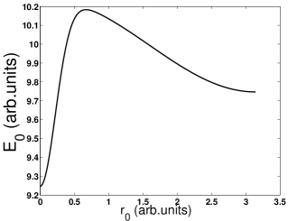
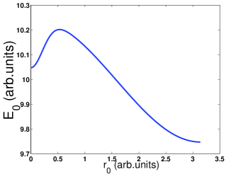
Figure 3: The minimum value of the energy functional $E$ as a function of $r_{0}$, Eq.(24) and Eq.(26), has two possible shapes. In the large $t$ limit it behaves like the upper one, and one may expect that it will eventually behave like the lower one as $t/U_{12}$ decreasing. In the following text we will discuss whether and when such a transition will take place.

From the $r_{0}$ dependence of the energy Eq.(24) and Eq.(26), one can easily find that the hopping energy favor a vanishing $r_{0}$ while $f(r_{0})$ favors a non-vanishing $r_{0}$. As schematically shown in Fig.(3) there possibly exist two local minima located at $r_{0}=0$ and $r_{0}=(b_{1}+b_{2})/3$. The true ground state is determined by comparing the two local minima, denoted by $E_{1}$ and $E_{2}$ respectively. In the large $t$ limit when the hopping energy is dominant, the ground state is at $\vec{r}_{0}=0$ as shown in the left side of Fig.(3). One may expect that $E_{1}$ will be eventually larger than $E_{2}$ as the right side one, and result in a first order transition of $r_{0}$ as $t/U_{12}$ decreasing.

At $r_{0}=(b_{1}+b_{2})/3$ the coherent terms are small enough and can be neglected, the minimum value of $E$ is therefore independent of $t$ and $\theta$. One can easily find out from Eq.(24) and Eq.(26) that

$$E_{2}=-\frac{3C}{2}\frac{AU_{12}}{\sqrt{I_{1}}U}.$$ (27)

We can also find from these two equations that $E_{1}$ increases as $t$ decreases, however there exists an upper bound, i.e.

$$E_{1}\leq\frac{AU_{12}}{\sqrt{I_{1}}U}3C-\frac{AU_{12}}{2U}\sqrt{I_{1}}.$$ (28)

For the phase transition taking place, it is required that $E_{1}>E_{2}$, i.e

$$9C>I_{1}.$$ (29)

This condition can not be satisfied for the triangular vortex lattice, where $I_{1}=1.1596$ and $C=0.0532$. Therefore, the conclusion is that the two sets of vortex lattices will coincide throughout all of the coherent regime.

As we have emphasized the underlying physics of the transition of $r_{0}$ is the competition between the coherent terms and the density-density interaction term. The coherent terms include one-particle hopping term $\varphi_{1}^{*}\varphi_{2}$, whose characteristic energy is $t$, and the two-particle hopping terms $\varphi_{1}^{*2}\varphi_{2}^{2}$, whose characteristic energy is $U_{12}$. When $t\gg U_{12}$ the relative phase $\theta$ between two layers will be zero, which is beneficial to one-particle hopping energy. We found that in this case the hopping energy will always dominate over the density-density interaction energy. With $t$ decreasing, $\theta$ will change from zero to $\pi/2$ to minimize the two-particle hopping energy. Eventually whether the transition can occur mostly depends on the competition between two-particle hopping term and the density-density interaction term. Since both these two terms share the same characteristic energy $U_{12}$, which term will be dominant relates to the intrinsic properties of the vortex lattice states. This can be seen from Eq.(29), where $I$ and $C$ only depend on the lattice structure.

Hence if the lattice type is changed, the above conclusion must consequently be changed. We will generalize the above discussion to arbitrary lattice type and find out on what condition the transition can occur in the fourth subsection.

III.3 Sliding Mode Frequency

Before continuing our discussion on the transition, in this subsection we discuss briefly one new excitation mode, which is unique to this system. This mode is characterized by small amplitude oscillation of $r_{0}$ around its equilibrium position $r_{0}=0$. We call this mode sliding mode because the vortices in one layer oscillate in locked steps relative to the other layer, and for the optical lattice case (see the right side of Fig.(1)) this mode can be corresponding to Kelvin mode of vortex line in the conventional three-dimensional rotating BEC.Stoof

We write down the propagate in the path integral representation as follows

$$Z=\int d\Psi^{*}d\Psi\exp\left[\frac{i}{\hbar}\int dtd^{2}ri\Psi^{*}\partial_{t}\Psi-E(\Psi^{*},\Psi)\right].$$ (30)

To consider the oscillation of $r_{0}$ we have

$$\Psi^{*}\partial_{t}\Psi=\Psi^{*}(\partial_{\delta r_{0}}\Psi)\delta\dot{r}_{0}=n_{2}\varphi_{2}^{*}(\partial_{r_{0}}\varphi_{2})\delta\dot{r}_{0},$$ (31)

the second equality follows from the fact that only $\varphi_{2}$ contains $r_{0}$. We notice that it is necessary to go beyond the mean field approximation and take the density fluctuation into account in order to obtain a dynamic term of $r_{0}$. The fluctuation of $n_{2}$ denoted by $\delta n$ contains two contributions. One comes from the inter-layer coupling, which is independent of spatial coordinates. The coupling to this part can not induce a dynamic term of $r_{0}$ because $\int d^{2}r\varphi^{*}\partial_{r_{0}}\varphi$ vanishes at $r_{0}=0$. Therefore in order to obtain a non-vanishing dynamic term we should include the intra-layer local density fluctuation bringing the condensate out of the lowest Landau levels. The dynamic term in Eq.(30) is then written as

$$\int dt\delta\dot{r}_{0}\int d^{2}r\delta{n}(r)i\varphi_{2}^{*}\partial_{r_{0}}\varphi_{2}.$$ (32)

We can then expand the energy functional around the saddle point to the second order, the result is

$$\delta^{2}E = \frac{t}{2}\cos\bar{\theta}N_{v}\frac{\pi}{v_{c}}\delta r_{0}^{2}-\frac{U}{\pi\sigma^{2}_{0}}I_{1}\cos 2\bar{\theta}N_{v}\frac{\pi}{2v_{c}}\delta r_{0}^{2}$$ (33)

$$+ \int d^{2}r4U|\varphi_{2}|^{4}\delta n(r)^{2}.$$

The term $f(r_{0})$ has been neglected in the above equation because the coefficient of second order expansion in the neighborhood of $r_{0}=0$ is relative small. Here $\sigma_{0}$ is the saddle point of $\sigma$. We first integrate the field $\delta n(r)$ out to obtain a dynamic term of $r_{0}$, the effective Lagrangian describing the oscillation of $r_{0}$ then reads

$$L=\int\frac{m_{\text{eff}}}{2}\delta\dot{r}_{0}^{2}-\frac{N_{v}\pi}{2v_{c}}\left[t\cos\bar{\theta}-\frac{UI_{1}\cos 2\bar{\theta}}{\pi\sigma^{2}_{0}}\right]\delta r_{0}^{2}.$$ (34)

Here $m_{\text{eff}}$ is the effective dynamic mass of the collectively oscillation motion defined by

$$m_{\text{eff}}=\int d^{2}r\frac{-(\varphi_{2}^{*}\partial_{r_{0}}\varphi_{2})^{2}}{8U|\varphi_{2}|^{4}}.$$ (35)

Hence the oscillation frequency is

$$\omega_{s}=\sqrt{\frac{N_{v}\pi}{v_{c}}\left[t\cos\bar{\theta}-\frac{UI_{1}\cos 2\bar{\theta}}{\pi\sigma^{2}_{0}}\right]\frac{1}{m_{\text{eff}}}}.$$ (36)

What should be emphasized here is that this frequency is a smooth function of $\cos\bar{\theta}$. As shown in the above section $\bar{\theta}$ will gradually change from zero to $\pi/2$ below the critical point $t/U_{12}=4A\sqrt{I_{1}}/U$. This leads to the key prediction of this subsection that the sliding mode frequency will consequently exhibit a second order discontinuity at the critical point.

III.4 General Lattice Type

To discuss a vortex lattice with arbitrary lattice structure, instead of Eq.(18) we define

$$f(r_{0})=2\sum\limits_{K_{01},K_{10},K_{1-1}}\left(\frac{g_{K}}{g_{0}}\right)^{2}\cos\vec{K}\cdot\vec{r_{0}},$$ (37)

and denote its minimum by $M$, the condition(29) for a transition in $r_{0}$ is then modified to

$$I_{1}-2-2M>0.$$ (38)

For flat lattice $g_{K_{1,-1}}$ is much larger than $g_{K_{0,1}}$ and $g_{K_{1,0}}$. As an example for the lattice with $\arg\tau=\pi/6$,

$$\left|\frac{g_{K_{1,-1}}}{g_{0}}\right|^{2}=\left|\frac{g_{K_{-1,1}}}{g_{0}}\right|^{2}=0.1857,$$ (39)

it is much larger than $|g_{K_{0,1}}/g_{0}|^{2}$ and $|g_{K_{1,0}}/g_{0}|^{2}$, which are both equal to $0.0019$. In this case the minimum of $f(r_{0})$ is approximately

$$M=-f(r_{0}=0)=1-I_{1},$$ (40)

which can be reached when $r_{0}=(b_{1}+b_{2})/4$.

Hence the condition Eq.(38) can be satisfied when the lattice is flat enough that satisfies $\arg\tau<0.6728$. The transition takes place when $E_{1}=E_{2}$, i.e.

$$\left(\frac{t}{U}\right)^{2}=\frac{U_{12}}{U}8(3I_{1}-4)\left(\frac{A}{U}\right)^{2}.$$ (41)

Here $A/U$ is a dimensionless parameter and can be tuned in a wide range. As an example, we show in Fig.(4) the transition line for a flat lattice with $\arg\tau=\pi/6$. In the upper side the vortices in two layers coincide with each other and the vortex lines are parallel to the $z$ axis. On the other side two sets of lattices are staggered, and the phase coherence between layers is lost.

Therefore to experimentally observe such a transition in QHMF regime, the first step is to produce a sufficient flat vortex lattice. Although so far most observed vortex lattices are triangular, it is still possible to achieve other lattice structure by using some special methods. Recently in Ref.MOktel the author shown within the LLL approximation that for a condensate with small number of vortices the lattice structure can be compressed to be quite flat due to the anisotropy of confinement potential.

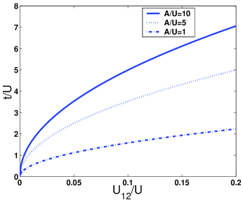
Figure 4: The phase boundary between $\vec{r}_{0}=0$ coherence regime and $\vec{r}_{0}\neq 0$ Fock regime, for different values of $A/U$. In the regime above the line $\vec{r}_{0}=0$ and below the line $\vec{r}_{0}\neq 0$, there is a first order transition when crossing the line.

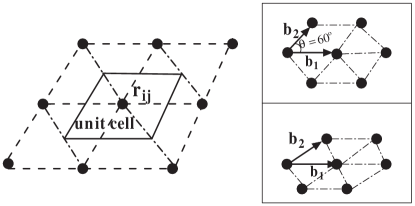
Figure 5: Left: The unit cell. Right: The schematic exhibition of triangular lattice and flat lattice.

III.5 Summarizes

In this section we have discussed the phase diagram of double-layer vortex lattice state, when both rotating condensates are in the QHMF regime. We summarize our results as follows and the phase diagram is shown in Fig.(6).

$1.$ In the coherent regime, for triangular lattice a transition of $\vec{r}_{0}$ is absent and $\vec{r}_{0}$ will always remain zero when the coherent hopping terms depending on the relative phase between two layers are introduced into the energy functional. When $t$ decreases the relative phase between two condensates will experience a second order change. The change of phase manifests itself in a second order change of the sliding mode frequency. The phase diagram is shown in the left side of Fig.(6)

$2.$ When the lattice is compressed to be quite flat, a transition of $r_{0}$ will occur when $U_{12}/t$ exceeds some critical value. The number fluctuation will be suppressed after the jumping of $r_{0}$ and a first order transition from the coherent regime to the Fock regime will be induced. It is noticed that such a transition from coherent regime to Fock regime is different from that discussed in the double-well BEC case, because it is driven by $t/U_{12}$ instead of $t/U$, and it is a first order transition instead of crossover. The phase diagram is shown in the right-side of Fig.(6)

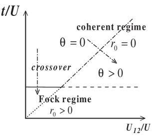
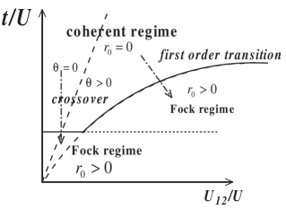
Figure 6: The phase diagram for the double-layer vortex lattice. The upper is for triangular lattice and the lower is for flat lattice

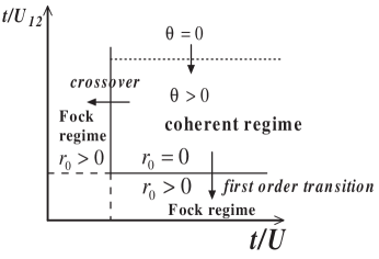
Figure 7: The phase diagram for the double-layer vortex lattice. This phase diagram is obtain when each rotating BEC is in Thomas-Fermi regime and the condition Eq.(58) is satisfied.

IV Thomas-Fermi Regime

We have mentioned that there are two different mean field descriptions of rotating BEC. In the last section we have focused on the QHMF regime. Before investigating the same issue when both condensates are in TFMF regime, we would like to have a brief discussion on the difference between two regimes.

As shown in the last section, QHMF works when the kinetic energy is much larger than the interaction energy. The wave functions are eigenstates of single particle Hamiltonian, and the mean value of $h_{xy}$ only depends on the average vortex density, and $\langle h_{x,y}\rangle$ neither depends on the winding number of each vortex nor the structure of vortex lattice. That the singly quantized vortices are arranged into triangular lattice is determined by taking the self-interaction energy into account. In contrast, TFMF is obtained by neglecting the kinetic energy, and the ground state density distribution is the result of the balance between effective trapping energy and interaction energy. The density distribution is assumed to be not remarkably changed and keeps a form of an inverted parabola when large number of vortices are contained. In this regime the interaction energy is independent of both the vortex winding number and the lattice structure. The kinetic energy caused by superfluid currents around the centers of vortices will induce an effective repulsive interaction between them. As a result the vortices are singly quantized and arrange into triangular lattice.

Besides there are also phenomenological differences between two regimes. In the TFMF regime the density profile is an inverted parabola and there exists a vortex core structure for each vortex. A vortex core structure means that there is a characteristic length $\xi$, inside which the superfluid density drops to zero rapidly, and outside which the superfluid density recovers the value free from vortices. Because the healing length increases as interaction strength decreases, when entering the QHMF regime $\xi$ is comparable to the inter-vortex spacing and no longer well defined. The individual vortex core structure disappears.

Therefore to deal with the TFMF regime we should use another wavefunction ansatz, which will be quite different from the one in QHMF regime. We know that the Thomas-Fermi density profile is

$$\rho_{0}(r)=\frac{1}{2g}\left(\mu-\frac{1}{2}m(\omega^{2}-\Omega^{2})r^{2}\right).$$ (42)

In the presence of vortex lattice we assume that the density profile is modified in the following way

$$\rho\propto\rho_{0}-\sum\limits_{r_{ij}}\rho_{o}(r_{ij})\exp\left(-\frac{(r-r_{ij})^{2}}{\xi^{2}}\right),$$ (43)

where $r_{ij}$ is the centers of vortices. $\xi$ is the vortex core side. Here we assume the $\xi$ is the same for all vortices. This ansatz is believed to be valid in the regime $\pi\xi^{2}<v_{c}\ll\pi R^{2}$, where $R$ is the Thomas-Fermi radius of the condensate.

We notice that

$$\int d^{2}\vec{r}\left[\rho_{0}-\sum\limits_{r_{ij}}\rho_{o}(r_{ij})\exp\left(-\frac{(r-r_{ij})^{2}}{\xi^{2}}\right)\right]$$

$$=1-\sum\limits_{r_{ij}}\rho_{0}(r_{ij})\pi\xi^{2},$$ (44)

in the large vortices limits, we can assume the area of a unit cell is much smaller than the size of condensate, approximately we have

$$\sum\limits_{r_{ij}}\rho_{0}(\vec{r}_{ij})v_{c}=\int d^{2}\vec{r}\rho_{0}(\vec{r})=1.$$ (45)

Hence Eq.(44) reduces to $1-\pi\xi^{2}/v_{c}$. Such approximation will be often used in the following derivation, the spirit of which is essentially keeping accuracy to the first order of $\pi\xi^{2}/v_{c}$ and neglecting $v_{c}/(\pi R^{2})$. Similar approach has also been used in Ref.Baym in the study of single component vortex lattice state.

The density distribution of vortex lattice state is

$$\rho=\frac{1}{1-\frac{\pi\xi^{2}}{v_{c}}}\left[\rho_{0}-\sum\limits_{r_{ij}}\rho_{o}(r_{ij})\exp\left(-\frac{(r-r_{ij})^{2}}{\xi^{2}}\right)\right],$$ (46)

and the wave function is written as

$$\varphi=\sqrt{\rho}\frac{f(z)}{|f(z)|}=\sqrt{\rho\frac{f(z)}{f(\bar{z})}}.$$ (47)

Here $f(z)=\prod\limits_{z_{ij}}(z-z_{ij})$ and can be described by the Jacobi theta function mentioned in the previous section.

In this regime, we can neglect the overlapping between vortex cores and then have

$$|\varphi_{1}(r)|^{2}|\varphi_{2}(r)|^{2}=\frac{1}{\left(1-\frac{\pi\xi^{2}}{v_{c}}\right)^{2}}\{\rho_{0}^{2}-$$

$$\sum\limits_{r_{ij}}\rho_{0}(r)\rho_{0}(r_{ij})e^{-(r-r_{ij})^{2}/\xi^{2}}$$

$$+\rho(r)\rho_{0}(r_{ij}+r_{0})e^{-(r-r_{ij}-r_{0})^{2}/\xi^{2}}$$

$$+\rho_{0}(r_{ij})\rho_{0}(r_{ij}+r_{0})e^{-[(r-r_{ij})^{2}+(r-r_{ij}-r_{0})^{2}]/\xi^{2}}\}.$$

Approximately we can assume $\rho_{0}(r_{ij}+r_{0})\simeq\rho_{0}(r_{ij})$ because $r_{0}$ is less than one lattice spacing and much smaller than the condensate size. Hence in Eq.(IV) only the last term involves $r_{0}$, explicitly

$$\int dxdy\sum\limits_{r_{ij}}\rho^{2}(r_{ij})e^{-[(r-r_{ij})^{2}+(r-r_{ij}-r_{0})^{2}]/\xi^{2}}$$ (49)

$$= \sum\limits_{r_{ij}}\rho^{2}(r_{ij})\frac{\pi\xi^{2}}{2}e^{-r_{0}^{2}/(2\xi^{2})}$$

$$\simeq \frac{\pi\xi^{2}}{2v_{c}}I_{2}\exp\left(-\frac{1}{2}\frac{r_{0}^{2}}{\xi^{2}}\right),$$

where $I_{2}$ is defined as $\int\rho_{0}^{2}d^{2}r$. And therefore

$$\int dxdy|\varphi_{1}|^{2}|\varphi_{2}|^{2}=\frac{1-2\frac{\pi\xi^{2}}{v_{c}}+\frac{\pi\xi^{2}}{2v_{c}}e^{-\frac{1}{2}\frac{r_{0}^{2}}{\xi^{2}}}}{\left(1-\frac{\pi\xi^{2}}{v_{c}}\right)^{2}}I_{2}.$$ (50)

We notice that the larger $r_{0}^{2}$, the smaller the density-density interaction energy. Hence its minimum is reached when $r_{0}=(b_{1}+b_{2})/2$.

Now we begin to discuss the coherent hopping terms in TF regime where

$$\varphi_{1}^{*}\varphi_{2}=\sqrt{\rho_{1}\rho_{2}}\sqrt{\frac{\varphi_{\text{qh}1}^{*}\varphi_{\text{qh}2}}{\bar{\varphi}_{\text{qh}{1}}\bar{\varphi}_{\text{qh}2}^{*}}}\ \ ,$$ (51)

using the result of Eq.(68) and taking the approximation of dropping all the terms with $K\neq 0$, we obtain that

$$\Re\varphi_{1}^{*}\varphi_{2}=\sqrt{\rho_{1}\rho_{2}}\cos\left(\frac{\pi}{v_{c}}\vec{r}\times\vec{r}_{0}\right),$$ (52)

and

$$\Im\varphi_{1}^{*}\varphi_{2}=\sqrt{\rho_{1}\rho_{2}}\sin\left(\frac{\pi}{v_{c}}\vec{r}\times\vec{r}_{0}\right).$$ (53)

From a careful analysis in the appendix(B) we conclude that at $r_{0}$=0

$$\Re\int dxdy\varphi_{1}^{*}\varphi_{2}=1,$$ (54)

and

$$\Re\int dxdy\varphi_{1}^{*2}\varphi_{2}^{2}=I_{2}\frac{1-\frac{3\pi\xi^{2}}{2v_{c}}}{(1-\frac{\pi\xi^{2}}{v_{c}})^{2}}=I_{3}.$$ (55)

Their imaginary parts vanish due to the spatial reflection symmetry. These coherent terms decrease as $r_{0}$ increases. When $r_{0}$ reaches its maximum value $(b_{1}+b_{2})/2$ these terms are small enough that can be neglected.

In the following we will find the ground state by comparing the minimum values of the energy function at $r_{0}=0$ and $r_{0}=(b_{1}+b_{2})/2$. We notice that at $r_{0}=0$

$$E=-\frac{t}{2}\cos\theta+4U_{12}I_{3}+2U_{12}\cos 2\theta I_{3}$$ (56)

and at $r_{0}=(b_{1}+b_{2})/2$,

$$E=4U_{12}I_{3}\frac{1-2\frac{\pi\xi^{2}}{v_{c}}}{1-\frac{3\pi\xi^{2}}{2v_{c}}}.$$ (57)

Following the similar procedure performed in the previous section, we find that when

$$\frac{\pi\xi^{2}}{v_{c}}>0.4$$ (58)

a transition of $r_{0}$ will occur as $t$ decreases. When the condition (58) is satisfied, the critical value of $t/U_{12}$ is

$$\frac{t}{U_{12}}=8I_{3}\sqrt{\frac{5\frac{\pi\xi^{2}}{v_{c}}-2}{1-\frac{3\pi\xi^{2}}{2v_{c}}}}.$$ (59)

When $t/U_{12}$ adiabatically decreases below this critical value, $r_{0}$ will jump from zero to a non-zero value, and the inter-layer quantum tunnelling will be suppressed immediately. The phase diagram is shown in Fig(7). It is physically similar to the right side of Fig.(6), but illustrated in an alternative way.

V Discussions and Conclusions

So far we have studied the phase diagram of double-layer rotating BEC in quantum Hall limit and Thomas-Fermi limit respectively. The complexity as illustrated in above discussions once again demonstrates the rich physics of rotating BEC and quantum coherence effect. Our model contains rich physics due to the four competing energies. The competition between intra-layer kinetic energy, whose characteristic value is $\hbar\Omega$, and the intra-layer interaction energy $U$ determines the properties of vortex lattice. The competition between inter-layer kinetic energy, whose characteristic value is $t$, and $U$ determines the phase fluctuation between layers. The effect of the competition between $t$ and $U_{12}$ is emphasized in this paper. However these three effects are entangled together and interact strongly with each other, that leads to the abundant physical phenomena.

What is most interesting is that under certain condition the system will exhibit a new kind of quantum phase transition as $t/U_{12}$ decreases. The transition is characterized by two sets of vortex lattice being staggered, and consequently the loss of phase coherence after the transition. Hence it presents a novel mechanism for superfluid to Mott transition. Furthermore, the condition that such a transition can happen depends on the intrinsic properties of each condensate. In TFMF regime, the condition is that the ratio of vortex core area to the area of unit cell should be larger than a critical value. While in QHMF regime the condition is that the lattice structure should be flat enough. We remark that the different criteria reflect the essential difference of these two physical regimes. Because how much energy the density-density interaction term can gain in the staggered lattices phase depends on the density undulation caused by vortices, in the TFMF regime the density undulation is mostly caused by vortex core structure. While in QHMF regime individual vortices cores are smeared, the density and phase singularities are strongly coupled, the density undulation therefore directly relies on how vortices arrange themselves. This indicates that the study of inter-layer coupling can be used as a powerful tool to reveal the intra-layer physics.

There are still many opening interesting questions. So far we still have no effective method to study the intermediate region between TFMF regime and QHMF regime, which may be relevant to the recent experiments of fast rotating BEC.CornellLLL Besides, if the rotating BEC is loaded into a one-dimensional optical trap, it is possible to achieve the regime that the atom number in each site is comparable to the vortex number, and in each layer the Bose atoms are strongly correlated.Ho2 Such a system may behave like a bosonic multi-layer fractional quantum Hall system. The discussion made in this model can also be applied to a rotating spin-$1/2$ condensate, with two hyperfine spin states coupled by photons. However in that case $U_{12}$ may be comparable with $U$, and the situation will be more complicated. More fruitful physics is expected in further investigation, and we hope that the theoretical results obtained in the present work will stimulate more experiments.

Acknowledgement  HZ would like to thank Professor C. N. Yang for his continuous encouragement and guidance. And the authors would like to acknowledge Professor T. L. Ho and Z. Y. Weng for helpful discussions. This work is supported by National Natural Science Foundation of China ( Grant No. 10247002 ) and the Ministry of Education of China.

Appendix A Calculation of Coherent Hopping Terms in QHMF Regime

In this appendix we will calculate the coherent hopping terms between two layers with the help of the Jacobi theta function in the QHMF regime. Using Eq.(9) we have

$$\theta^{*}(\zeta,\tau)\theta(\zeta+\bar{r}_{0},\tau)$$

$$=\sum\limits_{n_{1}=-\infty}^{+\infty}(-1)^{n_{1}}e^{-i\pi\tau^{*}(n_{1}+\frac{1}{2})^{2}+2\pi i\zeta^{*}(n_{1}+\frac{1}{2})}$$

$$\times\sum\limits_{n_{2}=-\infty}^{+\infty}(-1)^{n_{2}}e^{i\pi\tau(n_{2}+\frac{1}{2})^{2}+2\pi i\zeta(n_{2}+\frac{1}{2})}$$

$$=\sum\limits_{m_{1}}(-1)^{m}_{1}\exp[2\pi im_{1}\bar{x}-\frac{1}{2}v\pi m_{1}^{2}+i\pi(\bar{x}_{0}+i\bar{y}_{0})m_{1}]L_{m_{1}},$$

where $\bar{r}_{0}=r_{0}/b_{1}$, $m_{1}=n_{2}-n_{1}$ and $m^{\prime}=n_{1}+n_{2}+1$.

Here $L_{m_{1}}$ is explicitly written as

$$L_{m_{1}}=\sum\limits_{n_{1}=-\infty}^{+\infty}e^{i\pi um_{1}m^{\prime}-2\pi\bar{y}m^{\prime}-\frac{v}{2}\pi m^{\prime 2}+\pi i(\bar{x}_{0}+i\bar{y}_{0})m^{\prime}}$$

$$=\sum\limits_{m_{2}}\int dn_{1}e^{i\pi um_{1}m^{\prime}-2\pi\bar{y}m^{\prime}-\frac{v}{2}\pi m^{\prime 2}+\pi i(\bar{x}_{0}+i\bar{y}_{0})m^{\prime}}e^{2\pi im_{2}n_{1}}$$

$$=\sum\limits_{m_{2}}(-1)^{(m_{1}+1)m_{2}}\frac{1}{2}$$

$$\times\int dm^{\prime}e^{(i\pi um_{1}-2\pi\bar{y}+i\pi\bar{x}_{0}-\pi\bar{y}_{0}+i\pi m_{2})m^{\prime}-\frac{1}{2}v\pi m^{\prime 2}}$$

$$=\sum\limits_{m_{2}}\frac{1}{\sqrt{2v}}(-1)^{(m_{1}+1)m_{2}}e^{-\pi(m_{2}+\bar{x}_{0}+um_{1}+2i\bar{y}+i\bar{y}_{0})^{2}/2v}.$$

(61)

By defining

$$\vec{K}=\left[2\pi m_{1}\hat{x}-2\pi\frac{m_{2}+um_{1}}{v}\hat{y}\right]\frac{1}{b_{1}}$$ (62)

and

$$\vec{r}_{0}=\bar{x}_{0}\hat{x}+\bar{y}_{0}\hat{y},$$ (63)

we can verify that

$$\pi\bar{x}_{0}m_{1}-\pi\bar{y}_{0}(m_{2}+um_{1})/v=\frac{1}{2}\vec{r}_{0}\cdot\vec{K}$$ (64)

and

$$-\pi\bar{y}_{0}m_{1}-\pi\bar{x}_{0}(m_{2}+um_{1})/v=\frac{1}{2}\vec{r}_{0}\times\vec{K}.$$ (65)

Using Eq.(61),(64) and (65) we can obtain that

$$\theta^{*}(\zeta,\tau)\theta(\zeta+\bar{r}_{0},\tau)$$

$$=\sum\limits_{K}f_{K}e^{i\vec{K}\cdot\vec{r}}e^{\frac{\pi}{v}[2\bar{y}^{2}-2i\bar{y}(\bar{x}_{0}+i\bar{y}_{0})-(\bar{x}_{0}+i\bar{y}_{0})^{2}/2]},$$ (66)

where

$$f_{K}=\frac{(-1)^{m_{1}+m_{2}+m_{1}m_{2}}}{\sqrt{2v}}e^{\frac{1}{2}[(\vec{r}_{0}\times\vec{K})+i(\vec{r}_{0}\cdot\vec{K})]-v_{c}|K|^{2}/(8\pi)}.$$ (67)

Therefore

$$\varphi_{1}^{*}\varphi_{2}\propto\sum\limits_{K}f_{K}e^{i\vec{K}\cdot\vec{r}}\exp\left[-\frac{\pi}{2v}(2i\bar{y}+\bar{x}_{0}+i\bar{y}_{0})^{2}\right]$$

$$\times\exp\left[\pi\frac{w^{*2}+(w+r_{0})^{2}}{2v_{c}}-\frac{r^{2}+(r+r_{0})^{2}}{2a_{\perp}^{2}}\right]$$

$$=\sum\limits_{K}f_{K}e^{i\vec{K}\cdot\vec{r}}$$

$$\times\exp\left[-\frac{1}{\sigma^{2}}(r^{2}+\vec{r}\cdot\vec{r}_{0})-\frac{r_{0}^{2}}{2a_{\perp}^{2}}+\frac{\pi}{v_{c}}i(\vec{r}\times\vec{r}_{0})\right]$$ (68)

and

$$\varphi_{1}^{*2}\varphi_{2}^{2}\propto\sum\limits_{KK^{\prime}}f_{K}f_{K^{\prime}}e^{i(\vec{K}+\vec{K}^{\prime})\cdot\vec{r}}$$

$$\times\exp\left[-\frac{2}{\sigma^{2}}(r^{2}+r\cdot r_{0})-\frac{r_{0}^{2}}{a_{\perp}^{2}}+\frac{2\pi}{v_{c}}i(\vec{r}\times\vec{r}_{0})\right].$$

Then we can perform a integral over the two-dimensional space. After considering the normalized conditions, it yields

$$\int dxdy\varphi^{*}_{1}\varphi_{2}=$$

$$\frac{\sum\limits_{K}f_{K}e^{(\frac{1}{4\sigma^{2}}-\frac{\pi\sigma^{2}}{v_{c}}\frac{\pi}{v_{c}}-\frac{1}{2a_{\perp}})r_{0}^{2}+\frac{1}{2}\frac{\pi\sigma^{2}}{v_{c}}\vec{r_{o}}\times\vec{K}-\frac{\sigma^{2}|K|^{2}}{4}+i\vec{K}\cdot\vec{r_{0}}}}{\sum\limits_{K}g_{K}e^{-\frac{\sigma^{2}|K|^{2}}{4}}}.$$

(69)

Appendix B Calculation of Coherent Hopping Terms in the TFMF Regime

In this appendix we will calculate the energy of coherent hopping term in the TFMF regime. Begin with Eq.(52) we have

$$\Re\int d^{2}r\varphi_{1}^{*}\varphi_{2}=\sum\limits_{r_{ij}}\int\limits_{\text{unit cell}}d^{2}r\sqrt{\rho_{1}\rho_{2}}\cos[\frac{\pi}{v_{c}}(\vec{r}\times\vec{r}_{0})]=$$

$$\sum\limits_{r_{ij}}\int\limits_{\text{u.c}}d^{2}r\sqrt{\rho_{1}\rho_{2}}\cos[\frac{\pi}{v_{c}}(\vec{r}-\vec{r_{ij}})\times\vec{r}_{0}]\cos[\frac{\pi}{v_{c}}(\vec{r}_{ij}\times\vec{r}_{0})],$$

(70)

the $\sin$ term is cancelled out due to the spatial reflection symmetry.

Approximately in each unit cell we take

$$\rho_{1}=\frac{\rho_{0}(r_{ij})}{1-\frac{\pi\xi^{2}}{v_{c}}}[1-\exp\left(-\frac{(r-r_{ij})^{2}}{\xi^{2}}\right)]$$ (71)

and

$$\rho_{2}=\frac{\rho_{0}(r_{ij})}{1-\frac{\pi\xi^{2}}{v_{c}}}[1-\exp\left(-\frac{(r-r_{ij}-r_{0})^{2}}{\xi^{2}}\right)],$$ (72)

hence

$$\int\limits_{\text{u.c}}d^{2}r\sqrt{\rho_{1}\rho_{2}}\cos[\frac{\pi}{v_{c}}(\vec{r}-\vec{r_{ij}})\times\vec{r}_{0}]\frac{1-\frac{\pi\xi^{2}}{v_{c}}}{\rho_{0}(r_{ij})}=$$

$$\int\limits_{\text{u.c}}d^{2}r^{\prime}\sqrt{(1-e^{-\frac{r^{\prime 2}}{\xi^{2}}})(1-e^{-\frac{(r^{\prime}-r_{0})^{2}}{\xi^{2}}})}\cos[\frac{\pi}{v_{c}}\vec{r}^{\prime}\times\vec{r}_{0}]=$$

$$v_{c}\int\limits_{\text{u.c}}d^{2}r^{\prime}\sqrt{(1-e^{-\frac{r^{\prime 2}v_{c}}{\xi^{2}}})(1-e^{-\frac{(r^{\prime}-r_{0})^{2}v_{c}}{\xi^{2}}})}\cos[\pi\vec{r}^{\prime}\times\vec{r}_{0}].$$

(73)

Here $r^{\prime}$ is defined as $r-r_{ij}$. The second equality follows from a scaling that $r^{\prime}$ and $r_{0}$ are replaced by $r^{\prime}/\sqrt{v_{c}}$ and $r_{0}/\sqrt{v_{c}}$. We notice that for the determined lattice structure the integral in Eq.(73) only depends on $v_{c}/\xi^{2}$ and $r_{0}$, which is denoted as $F$ and can be obtained numerically.

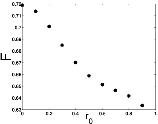
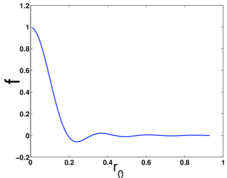
Figure 8: Upper: The integral $F$ as a function of $\frac{r_{0}}{\sqrt{v_{c}}}$. Lower: The integral $f$ as a function of $\frac{r_{0}}{\sqrt{v_{c}}}$. $v_{c}$ is set to unity, $T=\pi\xi^{2}/v_{c}$ is 0.3 and $N_{v}$ is 225.

Therefore

$$\text{Eq.(\ref{hoppingintegral1})}=\frac{F(\frac{v_{c}}{\xi^{2}},\frac{r_{0}}{\sqrt{v_{c}}})}{1-\frac{\pi\xi^{2}}{v_{c}}}\sum\limits_{r_{ij}}\rho_{0}(r_{ij})v_{c}\cos[\frac{\pi}{v_{c}}(\vec{r}_{ij}\times\vec{r}_{0})]$$

$$\cong\frac{F(\frac{v_{c}}{\xi^{2}},\frac{r_{0}}{\sqrt{v_{c}}})}{1-\frac{\pi\xi^{2}}{v_{c}}}\int drrd\theta\rho_{0}(r)\cos[\frac{\pi}{v_{c}}rr_{0}\sin\theta]$$

$$=2\pi\frac{F(\frac{v_{c}}{\xi^{2}},\frac{r_{0}}{\sqrt{v_{c}}})}{1-\frac{\pi\xi^{2}}{v_{c}}}\int drr\rho_{0}(r)J_{0}(\frac{\pi}{v_{c}}rr_{0}),$$ (74)

where $J_{0}$ is Bessel function of zero order. At $r_{0}=0$, $F$ equals to $1-\pi\xi^{2}/v_{c}$. As $r_{0}$ increases $F$ will decrease. The numerical result is shown in Fig.(8)

Besides, let $t=r/R$ with $R$ being the Thomas-Fermi radius we have

$$2\pi\int drr\rho_{0}(r)J_{0}(\frac{\pi}{v_{c}}rr_{0})$$

$$=\frac{\pi}{2g}m(\omega^{2}-\Omega^{2})R^{4}\int dtt(1-t^{2})J_{0}\left(\frac{\pi}{v_{c}}r_{0}Rt\right)$$

$$=\frac{8}{(\pi r_{0}R)^{2}/v_{c}^{2}}J_{2}\left(\frac{\pi r_{0}R}{v_{c}}\right).$$ (75)

The second equality follows from the Sonine integral identity and the fact that $\rho_{0}$ is normalized. It yields unit at $r_{0}=0$ and therefore Eq.(70) results in unit as we expected. Notice that

$$\frac{\pi r_{0}R}{v_{c}}=\sqrt{\frac{\pi R^{2}}{v_{c}}}\sqrt{\frac{\pi r_{0}^{2}}{v_{c}}}=\sqrt{N_{v}}\sqrt{\frac{\pi r_{0}^{2}}{v_{c}}},$$ (76)

where $N_{v}$ is the number of vortices contained in the cloud, and its typical value is $100\sim 250$ in current experiments. We choose $\sqrt{N_{v}}$ being $15$ in the following analysis, the result of Eq.(75) is therefore

$$\text{Eq.(\ref{BesselJ2})}=\frac{8}{225\sqrt{\pi}}\frac{1}{r_{0}^{2}/v_{c}}J_{2}\left(15\sqrt{\pi}\frac{r_{0}}{\sqrt{v_{c}}}\right).$$ (77)

Denoting the righthand side of Eq.(77) by $f$, $f$ as a function of $r_{0}/\sqrt{v_{c}}$ is plotted in the righthand side of Fig.(8). We find that $f$ is of the order $10^{-4}$ and the hopping energy can be neglected when $r_{0}=(b_{1}+b_{2})/2$.

In the same way we can calculate the two-particle hopping energy,

$$\Re\int dxdy\varphi_{1}^{*2}\varphi_{2}^{2}=\frac{2\pi W(\frac{v_{c}}{\xi^{2}},\frac{r_{0}}{\sqrt{v_{c}}})}{\left(1-\frac{\pi\xi^{2}}{v_{c}}\right)^{2}}\int drr\rho_{0}^{2}J_{0}\left(\frac{2\pi}{v_{c}}rr_{0}\right)$$

$$=\frac{2\pi W(\frac{v_{c}}{\xi^{2}},\frac{r_{0}}{\sqrt{v_{c}}})}{\left(1-\frac{\pi\xi^{2}}{v_{c}}\right)^{2}}\frac{64}{\pi R^{2}(2\pi r_{0}R/v_{c})^{3}}J_{3}\left(\frac{2\pi r_{0}R}{v_{c}}\right),$$ (78)

where $W$ function is defined as the integral

$$\int\limits_{\text{u.c}}d^{2}r(1-e^{-\frac{r^{2}\xi^{2}}{v_{c}}})(1-e^{-\frac{(r-r_{0})^{2}\xi^{2}}{v_{c}}})\cos\left(2\pi\vec{r}\times\vec{r}_{0}\right).$$ (79)

Similarly when $r_{0}=(b_{1}+b_{2})/2$ Eq.(78) is about of the order $10^{-8}$ and need not be considered.

References

- (1) M. Greiner, O. Mandel, T. Esslinger, T. W. Hsch and I. Bloch, Nature 415 39 (2001)
- (2) A. J. Leggett, Rev. Mod. Phys. 73, 307 (2001)
- (3) J. R. Abo-Shaeer, C. Raman, J. M. Vogels, W. Ketterle, Science 292, 476 (2001)
- (4) P. Engels, I. Coddington, P. C. Haljan, and E. A. Cornell, Phys. Rev. Lett. 89, 100403 (2002)
- (5) T. L. Ho, Phys. Rev. Lett. 87, 060403 (2001)
- (6) E. J. Mueller and T. L. Ho, Phys. Rev. Lett. 88, 180403 (2002)
- (7) K. Kasamatsu, M. Tsubota, and M. Ueda, Phys. Rev. Lett. 91, 150406 (2003)
- (8) Y. Shin, M. Saba, T. A. Pasquini, W. Ketterle, D. E. Pritchard, and A. E. Leanhardt, Phys. Rev. Lett. 92, 050405 (2004), and Y. Shin, M. Saba, A. Schirotzek, T. A. Pasquini, A. E. Leanhardt, D. E. Pritchard, and W. Ketterle Phys. Rev. Lett. 92, 150401 (2004)
- (9) T. G. Tiecke, M. Kemmann, Ch. Buggle, I. Shvarchuck, W. von Klitzing and J. T. M. Walraven, J. Opt. B: Quantum Semiclass. Opt. 5 S119 (2003)
- (10) The terms such as are neglected in the energy functional because they are smaller than the term and can be effectively absorbed into the term.
- (11) E. J. Mueller and T. L. Ho, Phys. Rev. A 67, 063602 (2003)
- (12) P. Engels, I. Coddington, P. C. Haljan, and E. A. Cornell, Phys. Rev. Lett. 89, 100403 (2002)
- (13) M. . Oktel, Phys. Rev. A 69, 023618 (2004)
- (14) J. P. Martikainen and H. T. C. Stoof, Phys. Rev. Lett. 91, 240403 (2003)
- (15) U. R. Fischer and G. Baym, Phys. Rev. Lett. 90, 140402 (2003)
- (16) V. Schweikhard, I. Coddington, P. Engels, V. P. Mogendorff, and E. A. Cornell, Phys. Rev. Lett. 92, 040404 (2004)
- (17) T. L. Ho and E. J. Mueller, Phys. Rev. Lett. 89, 050401 (2002)