Mesoscopic modelling of droplets
on topologically patterned substrates

Abstract

We present a lattice Boltzmann model to describe the spreading of droplets on topologically patterned substrates. We apply it to model superhydrophobic behaviour on surfaces covered by an array of micron-scale posts. We find that the patterning results in a substantial increase in contact angle, from $110^{o}$ to $156^{o}$.

1 Introduction

A droplet in contact with a substrate will try to spread to an equilibrium shape determined by Young’s law which describes the balance of surface tensions. There are many parameters which affect this process. For example surface disorder in the form of chemical or topological heterogeneities can pin a droplet or change its final shape. This has usually been viewed as a nuisance in experiments and applications. However with the advent of microfabrication techniques it is becoming possible to harness controlled surface topologies to explore new physical phenomena.

A beautiful example of this, inspired by the leaves of the lotus plant, is a superhydrophobic substrate. The angle $\theta$ between the tangent plane and the droplet is usually known as the contact angle. The higher the contact angle the more repellent the surface. There are applications, for example raincoats and windscreens, where repellent surfaces are highly desirable. Surface coatings and chemical modifications of the substrate are common ways to increase the contact angle but it is difficult to achieve an angle of more than $120^{o}$. However surfaces patterned with posts on a micron length scale allow contact angles of $160^{o}$ to be reached [1, 2].

Another example is nanopatterning of substrates which is of particular interest for the semiconductor industry. Applying a microstamp on a thin heated polymer film coating a substrate can create nanoscale patterns. The film dewets along the faces of the mold to form either thin lines or small patches. The present model has been used to simulate this new technique [3].

The aim of this paper is to present a lattice Boltzmann algorithm which can be used to investigate the behaviour of droplets on topologically patterned substrates. Lattice Boltzmann is a particularly appropriate approach in that it solves the Navier Stokes equations but also inputs the thermodynamic information such as surface tensions needed to describe the behaviour of droplets. Moreover its natural length scale, for fluids such as water, is of order microns where much of the exciting new physics is expected to appear. The method has already shown its capability in dealing with spreading on surfaces with chemical patterning [4].

In section 2 we summarise the algorithm and, particularly, describe the new thermodynamic and velocity boundary conditions needed to treat surfaces with topological patterning. In section 3 we present results for a substrate patterned by an array of posts. The patterning leads to a considerable increase in contact angle. Finally we discuss directions for future work using this approach.

2 The mesoscopic model

We consider a liquid-gas system of density $n(\mathbf{r})$ and volume $V$. The surface of the substrate is denoted by $S$. The equilibrium properties are described by the free energy

$$\Psi=\int_{V}\left(\psi_{b}(n)+\frac{\kappa}{2}\left(\partial_{\alpha}n\right)^{2}\right)dV+\int_{S}\psi_{c}(n)\;dS.$$ (1)

$\psi_{b}(n)$ is the free energy in the bulk. We choose a Van der Waals form

$$\psi_{b}(n)=p_{c}\left(\nu_{n}+1\right)^{2}(\nu_{n}^{2}-2\nu_{n}+3-2\beta\tau_{w})$$ (2)

where $\nu_{n}=(n-n_{c})/n_{c}$, $\tau_{w}=(T_{c}-T)/T_{c}$ and $p_{c}=1/8$, $n_{c}=7/2$ and $T_{c}=4/7$ are the critical pressure, density and temperature respectively and $\beta$ is a constant typically equal to $0.1$. The bulk pressure

$$p_{b}=p_{c}(\nu_{n}+1)^{2}(3\nu_{n}^{2}-2\nu_{n}+1-2\beta\tau_{w}).$$ (3)

The derivative term in equation (1) models the free energy associated with an interface. $\kappa$ is related to the surface tension. $\psi_{c}(n_{s})=\phi_{0}-\phi_{1}n_{s}+\cdots$ is the Cahn surface free energy [5] which controls the wetting properties of the fluid.

The lattice Boltzmann algorithm solves the Navier-Stokes equations for this system. Because interfaces appear naturally within the model it is particularly well suited to looking at the behaviour of moving drops.

2.1 The Lattice Boltzmann algorithm

The lattice Boltzmann approach follows the evolution of partial distribution functions $f_{i}$ on a regular, $d$-dimensional lattice formed of sites $\mathbf{r}$. The label $i$ denotes velocity directions and runs between $0$ and $z$. $DdQz+1$ is a standard lattice topology classification. The $D3Q15$ lattice we use here has the following velocity vectors $\mathbf{v}_{i}$: $(0,0,0)$, $(\pm 1,\pm 1,\pm 1)$, $(\pm 1,0,0)$, $(0,\pm 1,0)$, $(0,0,\pm 1)$ in lattice units as shown in fig. 1.

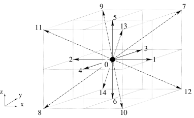
Figure 1: Topology of a $D3Q15$ lattice. The directions $i$ are numbered and correspond to the velocity vectors $\mathbf{v}_{i}$.

The lattice Boltzmann dynamics are given by

$$f_{i}(\mathbf{r}+\Delta t\mathbf{v}_{i},t+\Delta t)=f_{i}(\mathbf{r},t)+\frac{1}{\tau}\left(f_{i}^{eq}(\mathbf{r},t)-f_{i}(\mathbf{r},t)\right)$$ (4)

where $\Delta t$ is the time step of the simulation, $\tau$ the relaxation time and $f_{i}^{eq}$ the equilibrium distribution function which is a function of the density $n=\sum_{i=0}^{z}f_{i}$ and the fluid velocity $\mathbf{u}$, defined through the relation

$$n\mathbf{u}=\sum_{i=0}^{z}f_{i}\mathbf{v}_{i}.$$ (5)

The relaxation time tunes the kinematic viscosity as [6]

$$\nu=\frac{\Delta\mathbf{r}^{2}}{\Delta t}\frac{C_{4}}{C_{2}}(\tau-\frac{1}{2})$$ (6)

where $\Delta\mathbf{r}$ is the lattice spacing and $C_{2}$ and $C_{4}$ are coefficients related to the topology of the lattice. These are equal to $3$ and $1$ respectively when one considers a $D3Q15$ lattice (see [7] for more details).

It can be shown [8] that equation (4) reproduces the Navier-Stokes equations of a non-ideal gas if the local equilibrium functions are chosen as

$$f_{i}^{eq} = A_{\sigma}+B_{\sigma}u_{\alpha}v_{i\alpha}+C_{\sigma}\mathbf{u}^{2}+D_{\sigma}u_{\alpha}u_{\beta}v_{i\alpha}v_{i\beta}+G_{\sigma\alpha\beta}v_{i\alpha}v_{i\beta},\quad i>0,$$

$$f_{0}^{eq} = n-\sum_{i=1}^{z}f_{i}^{eq}$$ (7)

where Einstein notation is understood for the Cartesian labels $\alpha$ and $\beta$ (i.e. $v_{i\alpha}u_{\alpha}=\sum_{\alpha}v_{i\alpha}u_{\alpha}$) and where $\sigma$ labels velocities of different magnitude. A possible choice of the coefficients is [9]

$$A_{\sigma} = \frac{w_{\sigma}}{c^{2}}\left(p_{b}-\frac{\kappa}{2}(\partial_{\alpha}n)^{2}-\kappa n\partial_{\alpha\alpha}n+\nu u_{\alpha}\partial_{\alpha}n\right),$$

$$B_{\sigma} = \frac{w_{\sigma}n}{c^{2}},\quad C_{\sigma}=-\frac{w_{\sigma}n}{2c^{2}},\quad D_{\sigma}=\frac{3w_{\sigma}n}{2c^{4}},$$

$$G_{1\gamma\gamma} = \frac{1}{2c^{4}}\left(\kappa(\partial_{\gamma}n)^{2}+2\nu u_{\gamma}\partial_{\gamma}n\right),\quad G_{2\gamma\gamma}=0,$$

$$G_{2\gamma\delta} = \frac{1}{16c^{4}}\left(\kappa(\partial_{\gamma}n)(\partial_{\delta}n)+\nu(u_{\gamma}\partial_{\delta}n+u_{\delta}\partial_{\gamma}n)\right)$$ (8)

where $w_{1}=1/3$, $w_{2}=1/24$ and $c=\Delta\mathbf{r}/\Delta t$.

2.2 Wetting boundary conditions

The major challenge in dealing with patterned substrates is to handle the boundary conditions correctly. We consider first wetting boundary conditions which control the value of the density derivative and hence the contact angle. For flat substrates a boundary condition can be established by minimising the free energy (1) [5]

$$\hat{\mathbf{s}}\cdot\nabla n=-\frac{\phi_{1}}{\kappa}$$ (9)

where $\hat{\mathbf{s}}$ is the unit vector normal to the substrate. It is possible to obtain an expression relating $\phi_{1}$ to the contact angle $\theta$ as [9]

$$\phi_{1}=2\beta\tau_{w}\sqrt{2p_{c}\kappa}\;\mathrm{sign}\left(\frac{\pi}{2}-\theta\right)\sqrt{\cos\frac{\alpha}{3}\left(1-\cos\frac{\alpha}{3}\right)}$$ (10)

where $\alpha=\mathrm{cos}^{-1}(\sin^{2}\theta)$ and the function $\mathrm{sign}$ returns the sign of its argument.

Equation (9) is used to constrain the density derivative for sites on a flat part of the substrate. However, no such exact results are available for sites at edges or corners. We work on the principle that the wetting angle at such sites should be constrained as little as possible so that, in the limit of an increasingly fine mesh, it is determined by the contact angle of the neighbouring flat surfaces.

For edges (labels $9-12$ in fig. 2) and corners (labels $1-4$) at the top of the post each site has $6$ neighbours on the computational mesh. Therefore these sites can be treated as bulk sites.

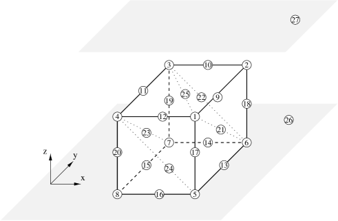
Figure 2: Sketch of a post on a substrate. Encircled numbers label sites in different topological positions. Labels $26$ and $27$ denote sites on the bottom ($z=z_{min}$) and the top ($z=z_{max}$) of the domain respectively.

At bottom edges where the post abuts the surface (labels $13-16$ in fig. 2) density derivatives in the two directions normal to the surface (e.g. $x$ and $z$ for sites labeled $13$) are calculated using

$$\partial_{z}n=\partial_{x/y}n=-\frac{1}{\sqrt{2}}\frac{\phi_{1}}{\kappa}$$ (11)

where the middle term constrains the density derivative in the appropriate direction $x$ or $y$.

At bottom corners where the post joins the surface (labels $5-8$ in fig. 2) density derivatives in both the $x$ and $y$ directions are known. Therefore these sites are treated as planar sites.

2.3 Velocity boundary conditions

We impose a no-slip boundary condition on the velocity. Because the collision operator (the right hand side of equation (4)) is applied at the boundary the usual bounce-back condition is not appropriate as it would not ensure mass conservation [10].

Indeed after applying equation (4) there are missing fields on the substrate sites because no fluid has been propagated from the solid. Missing fields are determined to fulfill the no-slip condition given by equation (5) with $\mathbf{u}=0$. This does not uniquely determine the $f_{i}$’s. For most of the cases (i.e. $1-20$) arbitrary choices guided by symmetry are used to close the system. This is no longer possible for sites $21-27$ where four asymmetrical choices are available. Selecting one of those solutions or using a simple algorithm which chooses one of them at random each time step leads to very comparable and symmetrical results. Hence we argue that an asymmetrical choice can be used. Possible conditions, which are used in the results reported here, are listed in table 1.

Label	Conditions
$1$	$f_{13}$	$=f_{14}$
$2$	$f_{7}$	$=f_{8}$
$3$	$f_{9}$	$=f_{10}$
$4$	$f_{11}$	$=f_{12}$
$5$	$f_{5}$	$=f_{6}$
	$f_{13}$	$=(f_{3}-f_{4}-f_{1}+f_{2})/2+f_{9}$
		$+f_{14}-f_{10}$
	$f_{11}$	$=(f_{1}-f_{2})/2-f_{9}+f_{10}+f_{12}$
	$f_{7}$	$=(-f_{3}+f_{4})/2+f_{8}-f_{9}+f_{10}$
$6$	$f_{5}$	$=f_{6}$
	$f_{13}$	$=(f_{3}-f_{4})/2-f_{11}+f_{12}+f_{14}$
	$f_{9}$	$=(f_{1}-f_{2})/2-f_{11}+f_{10}+f_{12}$
	$f_{7}$	$=(-f_{1}+f_{2}-f_{3}+f_{4})/2+f_{8}$
		$+f_{11}-f_{12}$
$7$	$f_{5}$	$=f_{6}$
	$f_{11}$	$=(f_{3}-f_{4})/2-f_{13}+f_{12}+f_{14}$
	$f_{9}$	$=(f_{1}-f_{2}-f_{3}+f_{4})/2+f_{13}$
		$-f_{14}+f_{10}$
	$f_{7}$	$=(-f_{1}+f_{2})/2+f_{8}-f_{13}+f_{14}$
$8$	$f_{5}$	$=f_{6}$
	$f_{11}$	$=(f_{3}-f_{4}+f_{1}-f_{2})/2+f_{7}$
		$-f_{8}+f_{12}$
	$f_{9}$	$=(-f_{3}+f_{4})/2-f_{7}+f_{8}+f_{10}$
	$f_{13}$	$=(-f_{1}+f_{2})/2-f_{7}+f_{8}+f_{14}$
$9$	$f_{13}$	$=f_{14}\quad;\quad f_{7}=f_{8}$
$10$	$f_{9}$	$=f_{10}\quad;\quad f_{7}=f_{8}$
$11$	$f_{9}$	$=f_{10}\quad;\quad f_{11}=f_{12}$
$12$	$f_{13}$	$=f_{14}\quad;\quad f_{11}=f_{12}$
$13$	$f_{5}$	$=f_{6}$
	$f_{1}$	$=2(-f_{10}+f_{9}+f_{11}-f_{12})+f_{2}$
	$f_{13}$	$=(f_{3}-f_{4})/2-f_{11}+f_{12}+f_{14}$
	$f_{7}$	$=(-f_{3}+f_{4})/2+f_{8}-f_{9}+f_{10}$
$14$	$f_{5}$	$=f_{6}$
	$f_{9}$	$=(f_{1}-f_{2})/2-f_{11}+f_{10}+f_{12}$
	$f_{7}$	$=(-f_{1}+f_{2})/2+f_{8}-f_{13}+f_{14}$
	$f_{3}$	$=2(-f_{12}+f_{11}+f_{13}-f_{14})+f_{4}$
$15$	$f_{5}$	$=f_{6}$
	$f_{2}$	$=2(-f_{14}+f_{7}+f_{13}-f_{8})+f_{1}$
	$f_{11}$	$=(f_{3}-f_{4})/2-f_{13}+f_{12}+f_{14}$
	$f_{9}$	$=(-f_{3}+f_{4})/2+f_{8}-f_{7}+f_{10}$

Label	Conditions
$16$	$f_{5}$	$=f_{6}$
	$f_{11}$	$=(f_{1}-f_{2})/2-f_{9}+f_{10}+f_{12}$
	$f_{13}$	$=(-f_{1}+f_{2})/2-f_{7}+f_{8}+f_{14}$
	$f_{4}$	$=2(-f_{10}+f_{7}+f_{9}-f_{8})+f_{3}$
$17$	$f_{10}$	$=f_{9}\quad;\quad f_{13}=f_{14}$
$18$	$f_{7}$	$=f_{8}\quad;\quad f_{12}=f_{11}$
$19$	$f_{9}$	$=f_{10}\;\;;\quad f_{14}=f_{13}$
$20$	$f_{8}$	$=f_{7}\quad;\quad f_{11}=f_{12}$
$21$	$f_{1}$	$=f_{2}\quad;\quad f_{7}=f_{8}$
	$f_{12}$	$=(-f_{3}+f_{4})/2+f_{11}$
	$f_{13}$	$=(-f_{5}+f_{6})/2+f_{14}$
	$f_{10}$	$=(f_{3}-f_{4}+f_{5}-f_{6})/2+f_{9}$
$22$	$f_{3}$	$=f_{4}\quad;\quad f_{7}=f_{8}$
	$f_{9}$	$=(-f_{5}+f_{6})/2+f_{10}$
	$f_{14}$	$=(f_{1}-f_{2}+f_{5}-f_{6})/2+f_{13}$
	$f_{12}$	$=(-f_{1}+f_{2})/2+f_{11}$
$23$	$f_{2}$	$=f_{1}\quad;\quad f_{8}=f_{7}$
	$f_{11}$	$=(f_{3}-f_{4})/2+f_{12}$
	$f_{14}$	$=(f_{5}-f_{6})/2+f_{13}$
	$f_{9}$	$=f_{10}+(-f_{3}+f_{4}-f_{5}+f_{6})/2$
$24$	$f_{8}$	$=f_{7}\quad;\quad f_{4}=f_{3}$
	$f_{11}$	$=(f_{1}-f_{2})/2+f_{12}$
	$f_{10}$	$=(f_{5}-f_{6})/2+f_{9}$
	$f_{13}$	$=(-f_{5}+f_{6}-f_{1}+f_{2})/2+f_{14}$
$25$	$f_{7}$	$=f_{8}\quad;\quad f_{5}=f_{6}$
	$f_{11}$	$=(f_{1}-f_{2}+f_{3}-f_{4})/2+f_{12}$
	$f_{9}$	$=(-f_{3}+f_{4})/2+f_{10}$
	$f_{13}$	$=(-f_{1}+f_{2})/2+f_{14}$
$26$	$f_{7}$	$=f_{8}\quad;\quad f_{5}=f_{6}$
	$f_{11}$	$=(f_{1}-f_{2}+f_{3}-f_{4})/2+f_{12}$
	$f_{9}$	$=(-f_{3}+f_{4})/2+f_{10}$
	$f_{13}$	$=(-f_{1}+f_{2})/2+f_{14}$
$27$	$f_{6}$	$=f_{5}\quad;\quad f_{8}=f_{7}$
	$f_{10}$	$=(f_{3}-f_{4})/2+f_{9}$
	$f_{14}$	$=(f_{1}-f_{2})/2+f_{13}$
	$f_{12}$	$=-(-f_{3}+f_{4}-f_{1}+f_{2})/2+f_{11}$

Table 1: Velocity boundary conditions.

The conservation of mass is ensured by setting a suitable rest field, $f_{0}$, equal to the difference between the density of the missing fields and the one of the fields entering the solid after collision.

3 Results

As an example we consider here the superhydrophobic behaviour of droplet spreading on a substrate patterned by square posts arranged as in fig. 3.

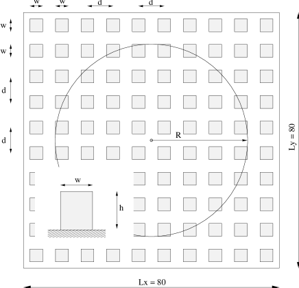
Figure 3: Sketch of the substrate. Dimensions are expressed in simulation units. Shaded areas are posts.

The size of the domain is $L_{x}\times L_{y}\times L_{z}=80\times 80\times 80$ and the height, spacing and width of posts are $h=5$, $d=8$ and $w=4$ respectively. A spherical droplet of radius $R=30$ is initially centered around the point $(x;y;z)=(41;41;36)$. The contact angle $\theta_{input}=110^{o}$ is set on every substrate site. The surface tension and the viscosity are tuned by choosing parameters $\kappa=0.002$ and $\tau=0.8$ respectively. The liquid density $n_{l}$ and gas density $n_{g}$ are set to $n_{l}=4.128$ and $n_{g}=2.913$ and the temperature $T=0.4$.

Fig. 4 shows the final state attained by the droplet for different substrates and initial conditions. For comparison fig. 4(a) shows a planar substrate. The equilibrium contact angle is $\theta_{a}=110^{o}=\theta_{input}$ as expected [9]. In fig. 4(b) the substrate is patterned and the initial velocity of the drop is zero. Now the contact angle is $\theta_{b}=156^{o}$, a demonstration of superhydrophobic behaviour. Fig. 4(c) reports an identical geometry but a drop with an initial impact velocity. Now the drop is able to collapse onto the substrate and the final angle is $\theta_{b}=130^{o}$. These angles are compatible with the ones reported in [2] where similar parameters are considered.

(a)
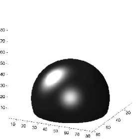
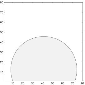
(b)
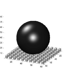
(c)

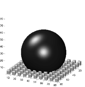
Figure 4: Final states of a spreading droplet. The right column reports cuts at $y=41$. (a) The substrate is flat and homogeneous. (b) The substrate is decorated with posts and the initial velocity of the droplet is $0$. (c) Same geometry as (b) but the droplet reaches the substrate with a velocity $0.01\Delta\mathbf{r}/\Delta t$. Each of these simulations ran for approximately 8 hours on 8 processors on a PC cluster.

For the parameter values used in these simulations the state with the droplet suspended on the posts has a slightly higher free energy than the collapsed state. It is a metastable state and the droplet needs an impact velocity to reach the true thermodynamic ground state. For macroscopic drops gravity will also be important in determining whether the drop remains suspended on top of the posts. Extrand has predicted the minimum post perimeter density necessary for a droplet to be suspended [11]. A next step will be to add gravity to the simulation to compare to his prediction.

Superhydrophobicity occurs over a wide range of $d$, the distance between the posts. For suspended drops of this size and $d\geq 12$ the drop resides on a single post and the contact angle is $170^{o}$. For $d<12$ the contact angle lies between $148^{o}$ and $156^{o}$ with the range primarly due to the commensurability between drop radius and post spacing.

It is of course also of interest to look further at the dynamics of the spreading. The droplet random motion reported in [2] and the bouncing back of droplets on nanotubes [12] pose many interesting directions for future research.

4 Conclusion

We have proposed a lattice Boltzmann model describing the spreading of a droplet on topologically patterned substrates. As an example, we have considered a substrate patterned with posts and found superhydrophobic behaviour in agreement with experiments [1, 2].

The algorithm gives us the capability to explore a wide variety of interesting problems concerning droplet behaviour on novel substrates and in microfluidic devices.

References

• [1] J. Bico, C. Marzolin, and D. Quéré. Pearl drops. Eur. Phys. Lett., 47(2):220–226, 1999.
• [2] D. Öner and T.J. McCarthy. Ultrahydrophobic surfaces. Effects of topography length scales on wettability. Langmuir, 16:7777–7782, 2000.
• [3] H.-L. Zang, D.G. Bucknall, and A. Dupuis. Molded dewetting of polymer thin films for general purpose nano-patterning. Macromolecule, submitted.
• [4] J. Léopoldès, A. Dupuis, D.G. Bucknall, and J.M. Yeomans. Jetting micron-scale droplets onto chemically heterogeneous surfaces. Langmuir, 19(23):9818–9822, 2003.
• [5] J.W. Cahn. Critical point wetting. J. Chem. Phys., 66:3667–3672, 1977.
• [6] S. Succi. The Lattice Boltzmann Equation, For Fluid Dynamics and Beyond. Oxford University Press, 2001.
• [7] A. Dupuis. From a lattice Boltzmann model to a parallel and reusable implementation of a virtual river. PhD thesis, University of Geneva, June 2002. http://cui.unige.ch/spc/PhDs/aDupuisPhD/phd.html.
• [8] M.R. Swift, E. Orlandini, W.R. Osborn, and J.M. Yeomans. Lattice Boltzmann simulations of liquid-gas and binary fluid systems. Phys. Rev. E, 54:5051–5052, 1996.
• [9] A. Dupuis and J.M. Yeomans. Lattice Boltzmann modelling of droplets on chemically heterogeneous surfaces. Fut. Gen. Comp. Syst., in press.
• [10] B. Chopard and A. Dupuis. A mass conserving boundary condition for lattice Boltzmann models. Int. J. Mod. Phys. B (DSFD 2002 conference), 17:103–106, 2002.
• [11] C.W. Extrand. Model for contact angles and hysteresis on rough and ultraphobic surfaces. Langmuir, 18:7991–7999, 2002.
• [12] K.K.S. Lau, J. Bico, K.B.K. Teo, M. Chhowalla, G.A.J. Amaratunga, W.I. Milne, G.H. McKinley, and K.K. Gleason. Superhydrophobic carbon nanotube forests. Nano Lett., in press.