Glassy phases in Random Heteropolymers with correlated sequences

Abstract

We develop a new analytic approach for the study of lattice heteropolymers, and apply it to copolymers with correlated Markovian sequences. According to our analysis, heteropolymers present three different dense phases depending upon the temperature, the nature of the monomer interactions, and the sequence correlations: $(i)$ a liquid phase, $(ii)$ a “soft glass” phase, and $(iii)$ a “frozen glass” phase. The presence of the new intermediate “soft glass” phase is predicted for instance in the case of polyampholytes with sequences that favor the alternation of monomers.

Our approach is based on the cavity method, a refined Bethe Peierls approximation adapted to frustrated systems. It amounts to a mean field treatment in which the nearest neighbor correlations, which are crucial in the dense phases of heteropolymers, are handled exactly. This approach is powerful and versatile, it can be improved systematically and generalized to other polymeric systems.

I Introduction

In the last 20 years much effort has been devoted to the theoretical study of heteropolymers Heteropolymerreview ; SfatosShakhnovich97 . One of the main motivations was to understand the statistical physics of protein folding PolymerREM ; WolynesREM ; BryngelsonReview95 ; Proteinfoldingbook2 ; Onuchicreview ; Grosberg00 . Despite the insight that has been accumulated, the goal remains distant. On the one hand, most analytical studies have been limited to random bond models GarelOrland88 ; ShakhnovichGutin89c (in which the interaction energies of all the couples of monomers along the chain are independent random variables), or to uncorrelated random copolymer sequences GarelLeibler94 ; SfatosGutin93 . However, there are many indications that sequence correlations induced by natural selection play an important role for the folding and stability of proteins. On the other hand, in this difficult problem, analytic computations have to resort to some approximations which are not easy to control. It is thus important to have a variety of different techniques at hand in order to crosscheck the predictions.

In this paper we develop a new tool for the analytical study of heteropolymers, based on the cavity method as used in various frustrated systems (a short account of our results has appeared in MontanariMullerMezard03a ). We use this method to investigate the phase diagram of copolymers with Markovian sequences. Within our approach we find copolymers to exist in three distinct dense phases (apart from the diluted coil phase at high temperature) depending upon the structure of the interaction energy matrix, the sequence correlations and the temperature: $(i)$ The liquid globule phase in which distinct monomers are essentially uncorrelated and can freely rearrange within the globule (apart from obvious constraints on monomers that are close along the chain); $(ii)$ the “frozen glass” phase in which the polymer is stuck in one out of a few well-separated low-energy conformations; $(iii)$ a “soft glass” phase with broken ergodicity (in the thermodynamic limit) in which the thermodynamically relevant conformations form a continuum in configuration space. This last phase has never been predicted in an analytical computation (although such a possibility has been envisioned in phenomenological models PolymerGREM1 ; Grosberg00 , and a very similar phase seems to be present in the numerical results of CopolymerPhasedia on the dynamics of heteropolymers.). Albeit frustrated, it has a much larger entropy, and appears already at a smaller density than the usual “frozen glass” phase.

Some of the most successful tools used so far in the study of random heteropolymers are mean field approaches based on the replica method GarelOrland88 ; ShakhnovichGutin89c ; SfatosGutin93 . Crucial to these calculations was the identification of some relevant order parameter, and the proposition of a suitable Ansatz describing the phase transition in a coupled space of real space coordinates and replica indices. This type of approach is potentially very powerful, but it becomes quite complex for heteropolymers. On the one hand, it requires a physical intuition for identifying the relevant degrees of freedom and of their behavior. On the other hand, an Ansatz tailored to describe a certain type of physics may hide other, unexpected features.

Our cavity method consists in a refined version of the Bethe Peierls approximation. While this also represents a kind of mean-field approximation, it differs fundamentally from the previous ones. Applying the Bethe-Peierls approximation to lattice heteropolymers allows to describe self-consistently the frustration on a local microscopic level. This approach can be thought of as the first step in the series of cluster variational (or Kikuchi) approximations Kikuchi51 . Its general philosophy consists in keeping track of local correlations inside some small region exactly, while treating the external degrees of freedom as an environment whose statistical properties have to be determined self-consistently. In the Bethe approximation, the only correlations which are treated exactly are the ones between neighboring sites on the lattice. This is an improvement with respect to the naïve mean field that treats distinct sites as statistically independent. Moreover, it is the first of such approximations to be meaningful for polymers, since the backbone structure induces strong correlations between neighbors Nagle74 ; AguileraKikuchi1 ; AguileraKikuchi2 ; AguileraKikuchi3 ; AguileraKikuchi4 ; AguileraKikuchi5 . Another potential advantage of the cavity method is that it can be used for one given polymer, without the need to average over an ensemble of sequences as in the replica method. While in the present work we focus on ensemble-averaged properties, one should keep in mind this possibility which could lead to interesting algorithmic developments in the future. Finally, the refined Bethe-Peierls approximation is supposed to be exact on locally tree-like structures (e.g., on random graphs). This is an important feature: It allows one to set up the mean-field analysis in a mathematically well-defined way, and its predictions can be checked against numerical simulations on those random “mean-field” lattices for which the theory is expected to be exact.

Within our cavity method, any heteropolymer is found to undergo a glass transition at large enough densities. Two main schemes of glass transitions can occur, depending on the details of the sequence, each of them being associated with one of the types of glasses mentioned above.

The transition to the frozen glass phase is a discontinuous transition, which is called random first order, or one step replica symmetry breaking (1RSB) transition in the replica language. It corresponds to the type of transition which has been found in many previous studies, of which the Random Energy Model (REM) Derrida81 is the simplest archetype.

The transition to the soft glass phase is a continuous one, corresponding to full replica symmetry breaking (FRSB). This is more in line with recent scenarios proposing a freezing that proceeds gradually from small scales to larger and larger structures Copolymerdyn ; CopolymerIsing . In a series of papers exploiting a Gaussian variational technique to deal with the dynamics of heteropolymers, copolymers in particular, a much richer phase diagram was proposed, where the ultimate REM-like folding to a unique ground state is preceded by a less structured but still frustrated glassy phase Copolymerkinetics ; CopolymerPhasedia ; Timoshenko98 . As for the glass transition, the random copolymer was proposed to be in the same universality class as the Ising spin glass CopolymerIsing , which would imply a continuous transition with a full breaking of the replica symmetry.

Beside providing an alternative and well controlled analytical approach, our cavity analysis adds to the above pictures in that it highlights the dependence of the scenario to be expected on the correlations of the monomer sequences.

In order to keep the computations more transparent we avoid here the use of replicas (although it would be possible to write all of the ensemble-averaged cavity equations using replicas), but we keep to the traditional replica vocabulary of 1RSB and FRSB to denote the two types of transitions.

We will apply here the general method to treat Markov-correlated sequences. However, a much wider range of possible applications of this technique is open.

The paper is organized as follows: In Section II we define the lattice model and review the treatment of polymers in the grand canonical ensemble. We then introduce the basic ideas of the Bethe approximation and discuss the $\Theta$-collapse from the random coil to the liquid globule phase. Section III discusses the shortcomings of the liquid solution and generalizes the method to the case where many pure states exist (as typically in a glassy phase). In particular, we propose a set of local order parameters that allow to distinguish both theoretically and experimentally between two different types of glass transitions. In Section IV we describe some basic tools for analyzing the glass transition. We present a local stability criterion for the liquid phase and the 1RSB cavity equations which are used to describe the glassy phase. This formalism is illustrated in Section V by considering the exemplary cases of alternating sequences with attractive or repulsive interactions of like monomers.

It turns out that the two types of interactions imply very different phase transitions: either a continuously emerging “soft” glass phase or the “standard” discontinuous freezing transition. These two scenarios are found in the study of Markovian chains in Sec. VI. The properties of the strongly frozen phase is analyzed in Section VII by focusing on maximally compact conformations. We conclude with a summary of our results and a discussion of their relevance for protein folding. Several technical developments are included in the seven appendices.

II The cavity approach to heteropolymers

In this Section we describe the type of heteropolymer models which we shall study. We derive their phase diagram under the assumption that the polymer is “liquid” meaning that any statistically relevant conformation is dynamically accessible to the molecule. In replica jargon this corresponds to assuming replica symmetry. The next sections will render more precise the regions of the phase diagram where this liquid phase is stable and corresponds to the physically relevant state.

II.1 The lattice polymer model

Our starting point is the standard model of lattice polymers Go75 ; ChanDill89 , which we generalize for polymers living on a general graph ${\cal G}$. We denote by $i,j,\dots\in{\cal V}$ the vertices of ${\cal G}$ (with $|{\cal V}|=V$), and by $(i,j),\dots\in{\cal E}$ the edges of ${\cal G}$. Let $\underline{\omega}=(\omega_{1}\dots\omega_{N})$, $\omega_{a}\in{\cal V}$ denote a self-avoiding walk (SAW) of length $N$ on ${\cal G}$. The position of a monomer along the chain is denoted by $a,b,\dots\in\{1\dots N\}$, and we assume an interaction matrix $e_{ab}$ to be assigned. The corresponding energy reads:

$$H_{N}(\underline{\omega})=\sum_{(a,b)|(\omega_{a},\omega_{b})\in{\cal E}}\,e_{ab},$$ (1)

where the sum runs over couples of non-consecutive monomers which are nearest neighbors on the lattice.

The choice of the matrix $e_{ab}$ is crucial. The standard homopolymer model is recovered by setting $e_{ab}=e_{0}$. A popular model in heteropolymer studies is the random bond model ShakhnovichGutin89c which assumes the $e_{ab}$ to be independent identically distributed (i.i.d) quenched random variables. In this work we study the more realistic case where the interaction energies are determined by the underlying monomer sequence. The sequence will be given by $\{\sigma_{1},\dots,\sigma_{N}\}$, with $\sigma_{a}\in{\cal A}$ being the type of the monomer at position $a$ in the sequence. The interaction energy of two monomers is assumed to depend only upon the monomer type: $e_{ab}=E_{\sigma_{a}\sigma_{b}}$. In particular, we shall focus on copolymers (although the approach is general) where there are only two types of monomers: ${\cal A}=\{A,B\}$. Interaction matrices $E_{\sigma,\sigma^{\prime}}$ of particular interest are:

• The HP model. $A$ and $B$ monomers represent (respectively) hydrophobic and polar aminoacids, and the interaction matrix is chosen accordingly, e.g., $E_{AA}=-1$, $E_{AB}=E_{BB}=0$. This is a popular toy model for protein folding HPmodel .

• The polyampholyte. $A$ and $B$ are supposed to carry screened charges which suggests $E_{AA}=E_{BB}=+1$ and $E_{AB}=E_{BA}=-1$. Sometime we shall refer to this interaction matrix as the antiferromagnetic (AF) model.

• The symmetrized HP model. We take $E_{AA}=E_{BB}=-1$ and $E_{AB}=E_{BA}=+1$. This is the standard model for copolymers with monomers that have a tendency to segregate SfatosShakhnovich97 . We shall refer to it as the ferromagnetic (F) model.

As for the graph ${\cal G}$ we shall consider two particular cases: $(i)$ A $V$-sites portion of the $d$-dimensional cubic lattice. $(ii)$ A $V$-sites Bethe lattice, i.e., a random lattice with connectivity $(k+1)$. Its interest stems from the observation that, in the thermodynamic limit, our mean-field calculations are exact on such a graph.

Both for our analytical computations and for the simulations on the Bethe lattice we shall need to consider periodic sequences with period $L$: $\sigma_{i}=\sigma_{i+L}$. The complete sequence is therefore determined by its first period $(\sigma_{1}\dots\sigma_{L})$. Hereafter, we shall use the shorthand notation “monomer $a$” to refer to all monomers in positions $a+nL$ with integer $n$. Furthermore, monomer indices always should be read modulo $L$. We expect the non-periodic case to be recovered in the $L\to\infty$ limit, even if this limit is taken after the limit $N,V\to\infty$.

The random-bond model is obtained in the $|{\cal A}|=L\to\infty$ limit by setting $\sigma_{1}\neq\sigma_{2}\neq\dots\neq\sigma_{L}$, and taking the $E_{\sigma,\sigma^{\prime}}$ to be i.i.d. random variables.

In order to understand the influence of the correlations in the sequence of monomers, we shall consider Markovian random copolymer chains in the large $L$ limit. In these chains the probability of a monomer to be of a certain type depends only on the preceding monomer in the sequence. For the sake of simplicity we assume the two types of monomers to occur with the same frequencies. The statistical ensemble of the chains is then fully characterized by the probability $\pi\in[0,1]$ of a monomer to be of the same type as the preceding one.

We study the system at thermal equilibrium at a temperature $T=1/\beta$. We define a canonical free energy density as

$$-\beta\,f_{L}(\beta,\rho)=\lim_{\stackrel{{\scriptstyle N,V\to\infty}}{{N=\rho V}}}\frac{1}{V}{\mathbb{E}}_{\cal G}\log\left(\sum_{\underline{\omega}}\text{e}^{-\beta H_{N}(\underline{\omega})}\right)\,,$$ (2)

and its grand-canonical counterpart

$$-\beta\,\omega_{L}(\beta,\mu)=\lim_{V\to\infty}\frac{1}{V}{\mathbb{E}}_{\cal G}\log\left(\sum_{N\geq 0}\text{e}^{\beta\mu N}\sum_{\underline{\omega}}\text{e}^{-\beta H_{N}(\underline{\omega})}\right)\,,$$ (3)

where the expectation value ${\mathbb{E}}_{\cal G}$ is taken with respect to the graph ensemble (whenever ${\cal G}$ is a random graph). The $L\to\infty$ limit, and the expectation with respect to the sequence $(\sigma_{1}\dots\sigma_{L})$ are (eventually) taken afterwards.

The two free energies defined above satisfy the usual Legendre transform relation $\omega_{L}(\beta,\mu)=f_{L}(\beta,\rho)-\mu\rho$. In order to describe free polymers (in equilibrium with the solvent) the chemical potential has to be adjusted to the critical value $\mu_{c}$ such that $\omega_{L}(\mu_{c})=0$ DeGennes75 . In the grand-canonical picture this critical line corresponds to a phase transition between an infinitely diluted phase for $\mu<\mu_{c}$ and a dense phase with non-vanishing osmotic pressure for $\mu>\mu_{c}$. If this phase transition is continuous, the density on the coexistence line vanishes, while it is finite if the transition is first order. On this coexistence line, the tricritical point where the nature of the transition changes is nothing but the $\Theta$-point where the collapse of the unconstrained polymer takes place.

In a homopolymer, the above description captures the essential of the phase diagram Bethehomopolymer . However, in a heteropolymer, the low temperature dense phase will be strongly influenced by the sequence heterogeneity. Due to the connectivity of the polymer chain it is in general impossible to find a compact folding where all interactions are favorable. The system is frustrated, and a glass transition will take place at sufficiently low temperature.

II.2 The Bethe Peierls approximation

As already mentioned, the Bethe approximation is asymptotically exact on locally tree-like graphs. Following cavity0 , we define a Bethe lattice as a random lattice with fixed connectivity. Such a lattice is locally tree-like since the typical loop size diverges as $\log V$ with the lattice size. In order to handle the heteropolymer problem on a $d$-dimensional hypercubic lattice within the Bethe approximation, our approach idealizes the graph as a Bethe lattice with the same connectivity, $k+1=2d$.

The local tree structure of the graph can be exploited in a recursion procedure. Suppose for a moment that the lattice is a tree, and let us single out a single branch of the tree which is rooted at one ‘cavity site’ $0$ having only $k$ neighbors $i=1,..,k$. In the absence of $0$, the branch would become a collection of $k$ other branches, rooted at $i=1,..,k$. This structure allows for a recursive computation of the probabilities of the polymer’s conformations on the tree.

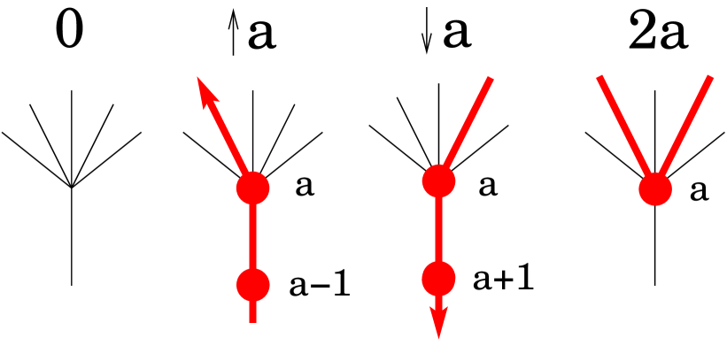
Figure 1: Possible conformations of a site (or oriented edge) on the regular Bethe lattice. The cavity site is considered as the root of a branch with $k$ leaves (here $k=5$). The thick lines and filled circles represent the chain backbone and monomers.

We first list the possible local conformations of the cavity site $0$ in its branch (see Fig. 1). $(0)$: the site is unoccupied; $(\uparrow a)$ or $(\downarrow a)$: the site is occupied by the monomer $a$ and the backbone continues towards the remainder of the tree, with monomer $a-1$ or $a+1$, respectively; $(2a)$: the site is occupied by monomer $a$, but the polymer returns back to the leafs. (On a real tree the parts of the polymer on different branches are necessarily disconnected. However, on the Bethe lattice this is no longer the case and the polymer may be present on more than two leaves.)

For each local conformation $\alpha\in\{0,\uparrow a,\downarrow a,2a\}$ of the root site $0$, we denote by $p_{\alpha}^{(0)}$ the corresponding probability (as given by the Boltzmann measure). The ($3L+1$) dimensional vector of weights ${\bf p}^{(0)}$, with components $p_{\alpha}^{(0)}$, can be expressed in terms of the corresponding $k$ weight vectors ${\bf p}^{(i)}$ on the neighboring sites. Note that $p_{\alpha}^{(i)}$ is the Boltzmann weight for the configuration $\alpha$ on $i$ when the site $0$ is absent. We will refer to these weight vectors on root-sites as cavity fields.

The mapping between cavity fields, ${\bf p}^{(0)}=I\left[{\bf p}^{(1)},...,{\bf p}^{(k)}\right]$, can be written explicitly as:

$$p_{0}^{(0)} = C^{-1}\prod_{i=1}^{k}\psi_{0}^{(i)},$$ (4)

$$p_{\uparrow a}^{(0)} = C^{-1}e^{\beta\mu}\sum_{i=1}^{k}p_{\uparrow a+1}^{(i)}\prod_{j\neq i}\psi_{a}^{(j)},$$ (5)

$$p_{\downarrow a}^{(0)} = C^{-1}e^{\beta\mu}\sum_{i=1}^{k}p_{\downarrow a-1}^{(i)}\prod_{j\neq i}\psi_{a}^{(j)},$$ (6)

$$p_{2a}^{(0)} = C^{-1}e^{\beta\mu}\sum_{i_{1}\neq i_{2}}p_{\downarrow a-1}^{(i_{1})}p_{\uparrow a+1}^{(i_{2})}\prod_{j\neq i_{1},i_{2}}\psi_{a}^{(j)},$$ (7)

where $C\equiv C[\{{\bf p}^{(i)}\}]$ is a normalization constant which enforces the condition $\sum_{\alpha}p^{(0)}_{\alpha}=1$ and we have introduced the quantities

$$\psi_{0}^{(i)}=p_{0}^{(i)}+\sum_{a^{\prime}=1}^{L}p_{2a^{\prime}}^{(i)}\,,\;\;\;\;\;\psi_{a}^{(j)}=p_{0}^{(j)}+\sum_{a^{\prime}=1}^{L}p_{2a^{\prime}}^{(j)}e^{-\beta e_{aa^{\prime}}}.$$ (8)

The full lattice is built by merging $k+1$ branches. Therefore, once the cavity fields have been computed, one can express any local quantity using the neighboring cavity fields. The monomer density $\rho^{(i)}$ at site $i$ is a function of the $k+1$ cavity fields ${\bf p}^{(j)}$ on the $j=1,...,k+1$ neighboring sites of $i$ (recall that ${\bf p}^{(j)}$ gives the probability of a local conformation on $j$ in the absence of $i$):

$$\rho^{(i)}=\sum_{a=1}^{L}\sum_{j_{1}\neq j_{2}}\frac{p^{(j_{1})}_{\uparrow a+1}p^{(j_{2})}_{\downarrow a-1}\prod_{j\neq j_{1},j_{2}}\psi^{(j)}_{a}}{w_{s}^{(i)}({\bf p}^{(1)},...,{\bf p}^{(k+1)})}\,,$$ (9)

where we have defined the normalization constant

$$w_{s}^{(i)}({\bf p}^{(1)},...,{\bf p}^{(k+1)}) = \prod_{j=1}^{k+1}\psi_{0}^{(j)}+e^{\beta\mu}\sum_{a=1}^{L}\sum_{j_{1}\neq j_{2}}p_{\downarrow a-1}^{(j_{1})}p_{\uparrow a+1}^{(j_{2})}\prod_{j\neq j_{1},j_{2}}\psi_{a}^{(j)}\,.$$ (10)

The internal energy $u_{ij}$ of a link $(i,j)$ can be written in terms of the cavity fields on $i$ and $j$ (giving the probabilities of local conformations on $i$ and $j$ in the absence of the link $(i,j)$):

$$u_{ij}=\sum_{a,b=1}^{L}e_{ab}\,n_{ij}(a,b)\,,\;\;\;\;\;\;\;n_{ij}(a,b)=\frac{p^{(i)}_{2a}p^{(j)}_{2b}\,\text{e}^{-\beta e_{ab}}}{w_{l}^{(ij)}({\bf p}^{(i)},{\bf p}^{(j)})}\,,$$ (11)

where $n_{ij}(a,b)$ is the probability of having a contact between two monomers $a$ and $b$ along the link $(ij)$ of the graph. The normalization $w_{l}({\bf p}^{(i)},{\bf p}^{(j)})$ is given by

$$w_{l}^{(ij)}({\bf p}^{(i)},{\bf p}^{(j)}) = p_{0}^{(i)}p_{0}^{(j)}+\sum_{a,b=1}^{L}p_{2a}^{(i)}p_{2b}^{(j)}\text{e}^{-\beta e_{ab}}+\sum_{a=1}^{L}\left(p_{0}^{(i)}p_{2a}^{(j)}+p_{2a}^{(i)}p_{0}^{(j)}+p_{\downarrow a-1}^{(i)}p_{\uparrow a}^{(j)}+p_{\uparrow a}^{(i)}p_{\downarrow a-1}^{(j)}\right)\,.$$ (12)

For each edge $(i,j)$ of a given graph, one can introduce a pair of cavity fields, describing respectively the probability of local configurations of the two points $i$ and $j$ in the absence of the edge $(i,j)$. One can write a Bethe free energy, which is a functional of all these cavity fields and has Eqs. (4)-(7) as stationarity conditions. It reads

$$V\beta\omega[\{{\bf p}^{(i)}\}]=-\sum_{i\in{\cal V}}\log[w_{s}^{(i)}]+\sum_{(ij)\in{\cal E}}\log[w_{l}^{(ij)}]\,,$$ (13)

where $w_{s}^{(i)}$ and $w_{l}^{(ij)}$ are the expressions given in (10) and (12), respectively. Notice moreover that the density (9) and the internal energy (11) can be obtained by differentiating the Bethe free energy with respect to the chemical potential $\mu$ and the inverse temperature $\beta$.

It is easy to show that the above expressions are exact if the graph ${\cal G}$ is a tree. On a general lattice it holds approximately to the extent that one can neglect the correlations between the fields on the $k+1$ neighbors of any site $i$, once the site $i$ itself has been deleted.

On a Bethe lattice, since the typical loop size diverges as $\log V$ in the large-$V$ limit, these $k+1$ sites neighbors of $i$ are generically distant from each other, when $i$ is absent. Therefore the correlations of their fields can be beglected, if the system is in a single pure state: at low temperature the Gibbs measure usually has to be decomposed into pure states, within which the correlations between two sites decay with their distance along the graph. We thus expect the above cavity approximation to become asymptotically exact, insofar as cavity fields are computed within one pure state.

II.3 The liquid solution and the $\Theta$-point

Both on the random Bethe lattice and on the $d$-dimensional cubic graph, each site has generically the same environment within any distance $R$ (as long as $R$ is kept finite in the $V\to\infty$ limit). A liquid phase is therefore expected to enjoy translational invariance and will be described by a set of fields $p^{(i)}_{\alpha}$ that is independent of the site. We thus look for a fixed point $p_{\alpha}^{(i)}\equiv p_{\alpha}^{*}$ of the recursions (4)-(7).

It turns out that the liquid solutions can be found by solving a system of $|{\cal A}|+2$ non-linear equations, $|{\cal A}|$ being the number of monomer species in the model. This is a great complexity reduction with respect to the $3L+1$ equations (4)-(7). The task can be further simplified by using particular symmetries of the interaction matrix. This is, for instance, the case of the F- and AF-models defined in Sec. II.1, which are symmetric under the interchange $A\leftrightarrow B$. We refer to App. A for a detailed discussion of how the solution is obtained.

As shown in Appendix A all the thermodynamic quantities depend upon the sequence $(\sigma_{1}\dots\sigma_{L})$ only through the fractions $\nu_{\sigma}$ of monomers of type $\sigma$. As a byproduct, the $L\to\infty$ limit can immediately be taken. The physical meaning of this result is easily understood. In the liquid phase, the correlations induced by the sequence play some role just along the chain, and their net effect vanishes at large distance. In particular, the monomer $a$ is surrounded by a certain fraction of monomers of type $\sigma^{\prime}$ which only depends on the type of $a$, $\sigma_{a}$ (apart from the sites occupied by the monomers $a-1$ and $a+1$, of course).

Let us now discuss the various solutions of liquid type.

The random coil phase is described by the trivial solution $p^{*}_{\alpha}=\delta_{\alpha,0}$, which exists for any choice of the parameters. This phase has vanishing grand potential $\omega$ and density $\rho$. At high temperatures this is the only solution when $\mu$ is smaller than the critical chemical potential $\mu_{c}$ given by $\exp(\beta\mu_{c})=1/k$. At $\mu_{c}$ a non-trivial solution emerges continuously. The latter describes a liquid phase under pressure ($\omega>0$ for $\mu>\mu_{c}$) with a density that vanishes on approaching the critical line.

The collapse of a free polymer from the random coil state to the liquid globule occurs at the so-called $\Theta$-point. In the grand-canonical description, it appears as the tricritical point on the line $\exp(\beta\mu)=1/k$. Expanding around $p^{*}_{\alpha}=\delta_{\alpha,0}$, one obtains the following relation which determines the $\Theta$-point temperature

$$\sum_{\sigma,\tau\in{\cal A}}\nu_{\sigma}\nu_{\tau}\,e^{-\beta_{\Theta}E_{\sigma\tau}}=\frac{k}{k-1}\,,$$ (14)

see App. A. This result has previously been obtained within the framework of the standard cluster variational method Pretti02 . At temperatures below the $\Theta$-point, $\beta>\beta_{\Theta}$, the grand-canonical phase transition becomes first order (see Fig. 2).

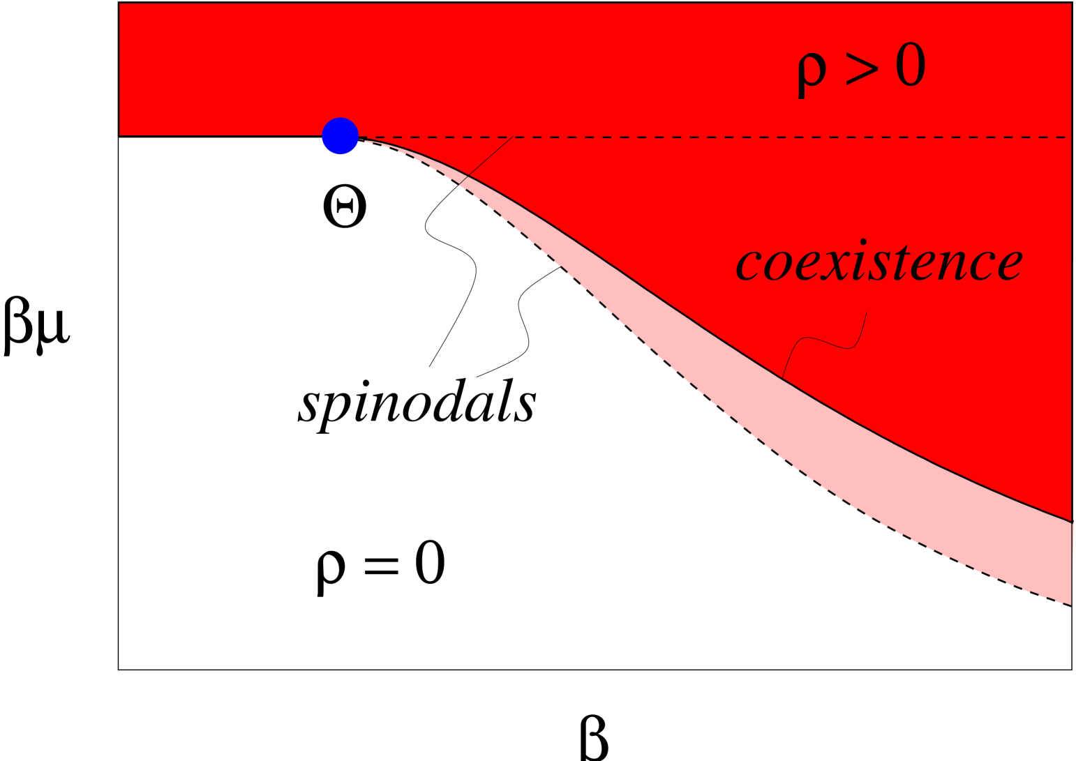
Figure 2: The phase diagram corresponding to the liquid (translation invariant) solution in the grand canonical ensemble. Above the $\Theta$-temperature, $\beta<\beta_{\Theta}$, the phase transition from the random coil phase ($\mu<\mu_{c}$) to the globule solution with finite density ($\mu>\mu_{c}$) is continuous. At low temperatures,$\beta>\beta_{\Theta}$ , the transition becomes first order and is accompanied by two spinodals. The globule solution on the critical line describes a free polymer in coexistence with the surrounding pure solvent. The free polymer undergoes a collapse transition at the $\Theta$-point

The critical line $\mu_{c}(\beta)$ is obtained by equating the grand potentials in the coil and globule phases, i.e., by solving $\omega=0$ for the globule solution. The density, internal energy, and free energy are obtained by plugging the globule solution $p^{*}_{\alpha}$ into Eqs. (9), (11), (13).

In the low temperature region $\beta>\beta_{\Theta}$, the dense solution can be continued to values of the chemical potentials smaller than the critical one $\mu_{\rm c}(\beta)$, and ceases to exist on a spinodal line.

Likewise, the trivial dilute solution stays locally stable beyond the coexistence line up to the spinodal $\exp(\beta\mu)=1/k$.

The above results compare reasonably with the outcomes of numerical simulations on $d$-dimensional lattice. For instance, the homopolymer $\Theta$-point on the cubic lattice given by $T_{\Theta}=1.50$ for $d=2$ GrassbergerHegger95b , $3.716(7)$ for $d=3$ TesiJanse96 , and $5.98(6)$ ($d=4$) PrellbergOwczarek00 . Moreover the authors of Ref. diamond found $T_{\Theta}=2.25(10)$ on the three-dimensional diamond lattice (connectivity $k+1=4$). These results should be compared with the outcome of the Bethe approximation, cf. (14), which yields $T_{\Theta,{\rm Bethe}}\approx 2.4663035$ (for $k=3$), $3.4760595$ ($k=4$), $4.4814201$ ($k=5$). $6.4871592$ ($k=7$). As for heteropolymers, the authors of Ref. KantorKardar94 ; GrassbergerHegger95 estimated $T_{\Theta}\approx 1.2$ both for the F- and AF-models of Sec. II.1 in $d=3$. This result is compatible with $T_{\Theta}=1/\log(2)\approx 1.442695$ which comes out of Eq. (14).

Finally, several numerical studies Monari99 ; BastollaGrassberger01 have focused on the $\Theta$-point of random bonds models, and have argued that its location is extremely well approximated by an annealed computation. Once again, this confirms that Eq. (14) is a reasonable approximation (the random-bond model is recovered by setting $|{\cal A}|=L$, $\nu_{\sigma}=1/L$ and $E_{\sigma\tau}$ i.i.d.’s random variables). This is also related to the numerical finding that the global collapse in protein folding dynamics is essentially unsensitive to the specific structure of the sequence, but only depends on its global composition BryngelsonReview95 .

III Glass phases

If we follow the entropy density $s(\beta)$ of the liquid solution as a function of temperature, we find that in any heterogeneous sequence $s(\beta)$ turns negative at sufficiently low temperatures. This indicates the existence of a phase transition to a glass phase which breaks the translational invariance.

As we will show, this glass transition can be of two types. In certain sequences the “entropy crisis” is preceded by a local instability of the cavity recursions (4)-(7) around the liquid fixed point $p^{*}_{\alpha}$. This implies the divergence of a properly defined spin-glass susceptibility and signals a continuous glass transition towards a phase with fully broken replica symmetry.

In other sequences, and in the Gaussian random bond model, this local instability is irrelevant since it occurs - if at all - in the region of negative entropy of the liquid globule. The glass transition is thus necessarily discontinuous (1RSB), as was predicted from replica calculations for the random bond model ShakhnovichGutin89a .

Dealing with the glass phases requires some modifications of the simple Bethe Peierls approximation which we have been using so far. In this section we will describe first some general properties of the glass phases, and explain the general technical tools that can be used to study glass transitions using the cavity method.

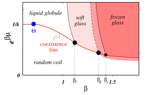
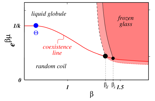
Figure 3: Schematic phase diagram of copolymers as a function of inverse temperature $\beta$ and chemical potential $\mu$. A polymer in equilibrium with the solvent is described by the coexistence line. Beyond the $\Theta$-point, $\beta>\beta_{\Theta}$ it is in a collapsed phase with a finite density. Depending on the sequence correlations of the copolymer there may be a local instability of the liquid (dash-dotted line), giving rise to a continuous glass transition at $\beta_{i}$ (see upper graph). In the absence of a local instability down to a critical temperature in the range of $\beta\approx 1.23$, a discontinuous glass transition will take place. The thermodynamic (static) phase transition at $\beta_{s}$ is preceded by a dynamic glass transition at $\beta_{d}$ where the phase space splits up into different pure states. In the glass phase, the critical chemical potential depends on whether the dynamically relevant threshold states (dashed line) or the states dominating the static equilibrium (solid line) are described.

III.1 Proliferation of pure states

In a glassy phase, the space of conformations is expected to split up in a multitude of pure states that are separated by large free energy barriers. The slowest time scale of the system, corresponding to jumps between pure states, increases dramatically.

In mean field approximation, or on the Bethe lattice, this time scale diverges and ergodicity is broken at the “dynamic” phase transition. The system eventually undergoes a “static” phase transition (with a non-analyticity in the thermodynamic potentials) at a lower temperature KirWol87 ; BouchaudCugliandolo98 .

In a finite-dimensional model the “dynamic” phase transition becomes a crossover where the nature of the most important dynamical processes changes. Whether the “static” phase transition survives in a given model, or not, is not known in general. We shall not enter this dispute here since we have little to say about it. In any case, the mean-field-like Bethe approximation, assuming the existence of many pure states, yields some useful insight on the glass phase.

Within one pure state, the conformational probabilities on a given site are well-defined cavityT ; cavity0 . However, there is no reason to assume the equality of local fields on different sites. Rather one expects that in a given pure state the sites will have different preferences for certain polymer conformations.

To proceed, one has to use a statistical description of local fields. We shall not explain here all the details of this description, but just give the main definitions and refer the reader to cavityT ; cavity0 for detailed discussions. In a glassy phase, the number of pure states $\mathcal{N}_{V}(\omega)$ increases exponentially with the volume of the system. The complexity $\Sigma(\omega)$ is the monotonously increasing, concave function defined by $\mathcal{N}_{V}(\omega)\sim\exp(V\Sigma(\omega))$. The natural order parameter is the distribution of local fields over the pure states $\gamma$ whose free energy density $\omega_{\gamma}$ is fixed to a value $\omega_{0}$:

$$\rho({\bf p})\propto\sum_{\gamma}\delta({\bf p}-{\bf p}^{(i,\gamma)})\delta(\omega_{\gamma}-\omega_{0}).$$ (15)

An alternative description consists in using a Legendre transformation of the complexity, by introducing the parameter $m=(1/\beta)\Sigma^{\prime}(\omega_{0})$ and working at fixed $m$ instead of fixed $\omega_{0}$ Monasson95 . This computation is equivalent to a 1RSB scheme with Parisi parameter $m$. From the free energy at fixed $m$, $\phi_{1}(m)$, the complexity $\Sigma(\omega)$ is obtained through the Legendre transform: $m\beta\phi_{1}(m)=m\beta\omega-\Sigma(\omega)$.

In a system with a discontinuous (1RSB) glass transition, this approach gives a full description. The complexity is strictly positive in the interval $\omega_{\rm s}<\omega<\omega_{\rm d}$, corresponding to the interval $m_{\rm d}<m<m_{\rm s}$ in the 1RSB parameter. The thermodynamically dominant metastable states are obtained by minimizing the one-replica free energy $\omega-\beta^{-1}\Sigma(\omega)$. In an intermediate temperature regime $T_{\rm s}<T<T_{\rm d}$, the minimum is attained for some free energy $\omega_{*}$ (corresponding to $m_{*}=1$), with $\omega_{\rm s}<\omega_{*}<\omega_{\rm d}$. Below the glass transition, $T<T_{\rm s}$, the minimum is attained at the lower edge $\omega_{*}=\omega_{\rm s}$ (with $\Sigma(\omega_{*})=0$), corresponding to the 1RSB parameter $0<m_{*}<1$.

In a system with a continuous glass transition (FRSB), the full solution should involve grouping states into clusters, and clusters into superclusters, building up a continuous ultrametric hierarchy. The approach above amounts to a 1RSB approximation of this full structure, and we shall not attempt to go beyond this level of approximation.

III.2 Order parameters

In this section we present two types of order parameters which can be used to identify the glass phase.

For a polymer in Euclidean space, described by the position $\vec{R}_{i}$ of monomer $i$, let us consider two replicas of the polymer in the same pure state. In the glass phase, provided the global rotation symmetry is broken, the local conformation of the two polymers will have a certain tendency to be the same while the liquid phase is completely disordered in this respect. In order to measure this effect, we introduce the scalar product of the distance vectors between nearby monomers in the replicas (1) and (2):

$$F_{d}^{(1,2)}=\sum_{i}(\vec{R}^{(1)}_{i+d}-\vec{R}^{(1)}_{i})\cdot(\vec{R}^{(2)}_{i+d}-\vec{R}^{(2)}_{i})\ .$$ (16)

We shall be interested in computing the average of this quantity when the replicas are constrained to remain in the same pure state. More precisely, we want to evaluate

$$\left\langle F_{d}^{(1,2)}\right\rangle_{\rm state}=\sum_{\gamma}w_{\gamma}\left\langle F_{d}^{(1,2)}\right\rangle_{1,2\in\gamma}\,,$$ (17)

where we average over all states $\gamma$ with their Boltzmann weigth $w_{\gamma}$. This quantity is accessible numerically. We consider a polymer which is thermalized at time $0$ in a configuration $\vec{R}_{i}(t=0)$. We let it evolve for a time $t$, to a configuration $\vec{R}_{i}(t)$. The order parameter is given by the quantity

$$\left\langle F_{d}^{(1,2)}\right\rangle_{\rm state}=\left\langle\frac{1}{t_{\rm MAX}}\int_{0}^{t_{\rm MAX}}dt\,\frac{1}{N}\sum_{i}(\vec{R}_{i+d}(t)-\vec{R}_{i}(t))\cdot(\vec{R}_{i+d}(0)-\vec{R}_{i}(0))\right\rangle_{\{R_{i}(t=0)\}}\,,$$ (18)

evaluated over timescales $t_{\rm MAX}$ which are large but much smaller than the typical timescale for interstate transitions or even full equilibration (in particular much smaller than the time scale for diffusion or rotation of the polymer, which diverges with $N$).

A simpler order parameter can be defined by first introducing, on each site $i$ of the lattice, the quantity $s_{i}$ which takes the value $s_{i}=1$ if the site is occupied by a monomer $A$, $s_{i}=-1$ if there is a $B$ monomer and $s_{i}=0$ if the site is empty. Then the overlap between two configurations 1 and 2 of the polymer can be defined as

$$q^{(1,2)}_{AB}=\frac{1}{V}\sum_{i=1}^{V}s^{(1)}_{i}s^{(2)}_{i}\,.$$ (19)

Again, one can compute the typical distance $\left\langle q^{(1,2)}_{AB}\right\rangle_{\rm state}$ between two conformations in the same state by recurring to dynamical simulations.

Notice that both $q^{(1,2)}_{AB}$ and $F_{d}^{(1,2)}$ define a notion of distance (or similarity) between polymer configurations. However, they describe two complementary aspects of the polymer: $q^{(1,2)}_{AB}$ essentially characterizes the bias of single sites towards a specific monomer type, whereas the order parameters $F_{d}^{(1,2)}$ measure the conformational similarity of the replicas in the vicinity of a given site, once the monomer on that site has been fixed. They measure the freezing of the local degrees of freedom of the polymer’s backbone, similarly to the approach of Copolymerkinetics ; CopolymerPhasedia ; Timoshenko98 . In contrast the parameter $q^{(1,2)}_{AB}$ is hardly sensitive to the geometric constraints induced by the backbone.

A dynamical evaluation of the above order parameters is particularly convenient on finite-dimensional lattices. Notice that the equilibrium probability for two independent replicas to have a finite overlap $q^{(1,2)}_{AB}$, vanishes with the volume of the lattice because of translation invariance.

On the Bethe lattice it is more natural to work at a finite monomer density, (see Sec. V.4). In this case, the random structure of the lattice acts as a “pinning field”, and two replicas of the same system typically have a finite overlap. Following the practice from spin-glass theory, we shall measure the probability distribution of the quantity (19) with respect to the Gibbs measure:

$$P_{AB}(q)=\left\langle\delta\left(q-q_{AB}^{(1,2)}\right)\right\rangle\,.$$ (20)

In a liquid phase, $\left\langle q^{(1,2)}_{AB}\right\rangle_{\rm state}$ vanishes and the function $P_{AB}(q)$ is a $\delta$-function. In a glass phase $\left\langle q^{(1,2)}_{AB}\right\rangle_{\rm state}>0$ and the function $P_{AB}(q)$ becomes non-trivial, with support in the interval $[-\left\langle q^{(1,2)}_{AB}\right\rangle_{\rm state},\left\langle q^{(1,2)}_{AB}\right\rangle_{\rm state}]$. In the case of a continuous transition, $\left\langle F^{(1,2)}_{d}\right\rangle_{\rm state}$ and $\left\langle q^{(1,2)}_{AB}\right\rangle_{\rm state}$ vanish at the transition point, while they exhibit a jump in the discontinuous case.

IV Methods to study the glass phases in the cavity approach

In this section we present the methods that we use to study the glass transition on the Bethe lattice. They are applied to various types of polymers in the next sections.

IV.1 Local instability towards a soft glass phase

The simplest glass transition is the one associated with an instability of the liquid. The liquid solution is always embedded in the 1RSB formalism as the single pure state that exists at high temperature: it is described by the field distribution $\rho({\bf p})=\delta({\bf p}-{\bf p}^{*})$. This solution becomes locally unstable if fluctuations around ${\bf p}^{*}$ grow on average under the cavity recursion (4-7). This phenomenon occurs when

$$k\lambda_{\rm max}^{2}\geq 1$$ (21)

where $\lambda_{\rm max}$ is the largest eigenvalue of the transfer matrix for the propagation of deviations from the liquid under the recursion (4)-(7),

$$\mathcal{M}_{\alpha\alpha^{\prime}}=\partial I_{\alpha}[{\bf p}^{(1)},\dots,{\bf p}^{(k)}]/\partial{p}^{(1)}_{\alpha^{\prime}}|_{{\bf p}^{(i)}={\bf p}^{*}}\,.$$ (22)

(Notice that the stronger instability $k|\lambda_{\rm max}|=1$ MPSdeGennes is irrelevant on a random lattice, since it is associated to the establishment of a crystalline order that is inherently frustrated because of the presence of large loops.) Beyond the local instability, the distribution of local fields $\rho({\bf p})$ becomes non-trivial, but it remains centered around the unstable liquid fixed point. In physical terms this indicates that phase space begins to divide up into a small number of states that comprise a large number of microconfigurations. These states are characterized by weak local preferences for certain polymer conformations that deviate only slightly from the homogeneous liquid state.

The instability (21) generally develops below a temperature $T_{i}$. Calling $T_{\rm cris}$ the temperature where the entropy vanishes, one can have two types of situations:

• When $T_{i}<T_{\rm cris}$, the local instability of the liquid is clearly irrelevant, and a discontinuous glass transition must take place at some temperature $\geq T_{\rm cris}$.

• When $T_{\rm cris}<T_{i}$, either the instability drives a continuous glass transition (as we will see in specific examples, this seems to be the generic case when the instability occurs in a region where the liquid entropy is still large), or there exists again a discontinuous glass transition taking place at temperatures $T>T_{i}$ and rendering the instability irrelevant. It is also possible, that a first continuous glass transition towards a slightly frustrated phase undergoes a successive discontinuous phase transition at lower temperatures where a stronger degree of freezing takes place.

Because of the relative simplicity of the liquid phase, it turns out that the stability condition (21) can be studied explicitly for AB copolymers with an interaction matrix which is symmetric under the $A\leftrightarrow B$ interchange. The detailed calculation is given in Appendix B. The dangerous eigenvalues $\lambda$ of the matrix $\cal M$ in (22) are found to obey the equation

$$\pm\frac{1}{k}\frac{w\sinh(\beta)}{1+w\cosh(\beta)}=\frac{\lambda(1-(k\lambda)^{-L})}{(k-2)+k(k\lambda)^{-L}+2(k-1)\sum_{i=1}^{L-1}q_{i}(k\lambda)^{-i}}\ ,$$ (23)

where the sign corresponds to ferromagnetic (+) and antiferromagnetic (-) interactions, respectively. The temperature dependent parameter $w=\sum_{a=1}^{L}p^{*}_{2a}/p^{*}_{0}$ characterizes the liquid solution and is independent of $L$, cf. App. A and Eqs. (47), (48). The sequence properties enter the above expression only through the autocorrelation function $q_{i}=(1/L)\sum_{a=1}^{L}\sigma_{a}\sigma_{a+i}$.

The local instability $\beta_{i}$ occurs at the smallest value of $\beta$ where the characteristic polynomial (23) has a root with $|\lambda|^{2}k=1$. Usually, for attractive interactions between equal monomers, the relevant eigenvalue is $\lambda=1/\sqrt{k}$ while the instability occurs in general with $\lambda=-1/\sqrt{k}$ in ampholytes.

The location of the instability for the various types of interactions and sequences will be studied in the next sections. Let us just mention here that the (periodic) Gaussian random bond heteropolymer generically undergoes a discontinuous 1RSB glass transition, in agreement with previous studies ShakhnovichGutin89c .

IV.2 Cavity recursion within the 1RSB approximation

In order to study the glass phase itself, we need to compute the distribution of local fields of (15) for the Bethe lattice. We shall do it here within the 1RSB cavity formalism of (cavity0 ; cavityT ). We shall not rederive the full formalism but give the main ingredients needed for our study. The statistical average of the simple cavity recursion (4-7), which holds within a given pure state, leads to a recursion relation for this distribution:

$$\rho({\bf p})=\frac{1}{\mathcal{Z}}\int\prod_{i=1}^{k}d\rho({\bf p}^{(i)})\;\delta({\bf p}-I[{\bf p}^{(1)},\dots,{\bf p}^{(k)}])\;e^{-m\beta\Delta f[{\bf p}^{(1)},\dots,{\bf p}^{(k)}]}$$ (24)

where $I[{\bf p}^{(1)},\dots,{\bf p}^{(k)}]$ is given by (4)-(7), and $\mathcal{Z}$ is a normalization. The non trivial reweighting, which depends on the parameter $m$ defined in Section III.1, involves the free energy change induced by the recursion, which is given by $\Delta f[\{{\bf p}^{(i)}\}]\equiv-\beta^{-1}\log(C[\{{\bf p}^{(i)}\}])$ , where $C[\{{\bf p}^{(i)}\}]$ is the normalization term appearing in (4)-(7). This reweighting accounts for the fact that the number of pure states increases exponentially with their free energy.

The free energy is obtained by properly weighting the contributions of different pure states:

$$\beta m\phi_{1}(m) = -\log\left[\int\prod_{i=1}^{k+1}\!d\rho({\bf p}^{(i)})\,w^{m}_{s}(\{{\bf p}^{(i)}\})\right]+\frac{k+1}{2}\log\left[\int\prod_{i=1}^{2}d\rho({\bf p}^{(i)})\,w^{m}_{l}({\bf p}^{(1)},{\bf p}^{(2)})\right]\,,$$ (25)

where $w_{s}$ and $w_{l}$ are the site and link partition functions defined in Eqs. (10) and (12). The complexity $\Sigma(\omega)$ is obtained from $\phi_{1}(m)$ through a Legendre transform: $m\beta\phi_{1}(m)=m\beta\omega-\Sigma(\omega)$. Note that the recursion relation (24) is the saddle point equation for the functional $\phi_{1}(m)$ with respect to $\rho({\bf p})$.

Close to a continuous glass transition, $\rho$ is strongly peaked around the liquid fixed point ${\bf p}^{*}$, and we can expand the free energy as a function of the moments of the fluctuations ${\bf p}-{\bf p}^{*}$ over the pure states, as outlined in Appendix D. To leading order the corrections to the liquid free energy arise from fluctuations in the “replicon” mode, the unstable direction of the transfer matrix (22), whose magnitude grows as $(T_{i}-T)^{1/2}$. The continuous glass transition is found to be of third order,

$$\phi_{1}-\phi_{\rm liq}=c\frac{1-m}{(2-m)^{2}}(T_{i}-T)^{3}+O\left((T_{i}-T)^{4}\right)$$ (26)

where $c$ is a positive constant. This is in contrast to discontinuous glass transitions which are (generally) of second order in the free energy.

V Two exemplary cases: The alternating ampholyte and HP model

In this section we apply the cavity 1RSB formalism to two specific sequences: the regularly alternating copolymer chains $ABABAB\dots$ for ampholytic and symmetrized-HP interactions. These turn out to be rather extreme representatives in the ensemble of possible neutral copolymers, but they are the simplest ones, and they exhibit the characteristics of the continuous (ampholyte) and discontinuous (HP) transition in a very clear manner.

The folding of an alternating copolymer on a regular Bethe lattice is a frustrated problem, while, clearly, on a regular cubic lattice, it would just behave as a homopolymer with homogeneous interactions $E_{AB}\equiv e$. However, we expect that as soon as a certain number of defects are introduced in such sequences, their folding on the cubic lattice will be similarly frustrated. In terms of Markovian sequences, we consider here the case of $\pi\ll 1$.

While these sequences are expected to behave differently from the alternating one $\pi=0$ on the cubic lattice, it is reasonable to assume that the $\pi\to 0$ limit is smooth on the Bethe lattice. Then the Bethe approximation of $\pi\ll 1$ sequences can be studied using the perfectly alternating sequence, as we do here here. Alternating chains are more easily studied with the cavity method, since the number of local fields may be reduced to 5 (with 4 independent degrees of freedom): due to the inversion symmetry the local conformations reduce to $\alpha\in\{0,1A,1B,2A,2B\}$, where $1A$ ($1B$) comprises the two conformations $\uparrow A$ and $\downarrow A$ ($\uparrow B$ and $\downarrow B$). The cavity recursion relation (24) can thus be handled relatively easily, using a population dynamics algorithm described in App. G

V.1 Ordered structures, correlations, frustration and the order of the glass transition

Before embarking on the details of the cavity computation for the alternating chains, we present here some simple arguments explaining the very different physical nature of the glass phase in the alternating ampholyte, which has a continuous transition, and in the symmetrized HP model, which has a discontinuous transition.

Instead of a Bethe lattice, let us consider a regular tree and ask for a maximally dense polymer configuration such that all interactions are satisfied ($AB$ interactions in ampholytes and $AA$ or $BB$ interactions in the symmetrized HP model). In Fig. 4 we show typical configurations for each case.

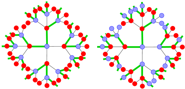
Figure 4: Unfrustrated, maximally dense structures on a tree ($k=3$). The ampholyte (left) has an evident stratified order and long range correlations of site occupancies. The location of $A$’s and $B$’s in the HP-polymer is correlated with the backbone configuration (thick edges) which makes the distribution of monomers look random.

While there is a stratified order in ampholytic configurations that manifests itself in strong long range correlations, the symmetrized HP model has an “ordered” structure that is highly correlated with the backbone configuration. No long range correlations may persist, and this dense ground state is difficult to distinguish from a dense liquid configuration.

If we turn back to a Bethe lattice, frustration is induced by the presence of large loops. Odd loops are inherently frustrated in the ampholyte since they necessarily have to break up the long range correlations of the layered structure. This is not the case in the HP-like model where most constraints from loops can be satisfied when the backbone is arranged in the right way. In other words, the information about local conformations and the associated constraints cannot be propagated far away in the case of the HP-like chain, since the correlations of ordered structures die out quickly with distance. As long as the density is not too large and there are sufficient voids in the globule, a global frustration will not be able to establish. For the ampholyte, however, it will be favorable, even at lower density, to develop local (site) preferences for a certain monomer type and thus increase the probability of satisfied interactions. This mechanism is at the basis of the instability of local fields in the liquid. Note that in the first place this instability is related to the type of monomer accommodated on a given site rather than the backbone structure. The latter will only come into play at larger densities/lower temperatures.

This qualitative discussion applies equally to correlated sequences which are not perfectly alternating but have a strong tendency to alternate (small $\pi$). At the other extreme, if one considers the case of $\pi$ close to one, where consecutive monomers tend to be alike, one can apply the same type of considerations, but with the roles of ampholyte and HP-like chain reversed. We can thus conclude that the local instability of a HP-like chain with long blocks of like monomers is associated to the appearance of pure states characterized by the same monomer preferences for small regions on the lattice. This is reminiscent of the microphase separation (MPS) Microphaseseparation which has been much discussed in this context and becomes relevant for sequences with a distinct block structure SfatosGutin93 ; GutinSfatos94 ; Dobrynin95 ; Heteropolymerreview . However one should remember that the present formulation of the cavity method, which neglects small loops in the lattice, does not allow any quantitative study of this phenomenon (this could be addressed using more refined cluster variational methods).

Repeating the above arguments for more general cases of short range correlated sequences, one sees that in general a local instability is favored by sequences whose monomer distribution tends to be annealed (e.g., ampholytes with a tendency towards charge alternation along the sequence). It is interesting to note that such ‘annealed sequences’ naturally result from common protein design schemes Sequencedesign1 ; Sequencedesign2 ; Copolymerdesign ; LevyFlight .

V.2 The continuous transition in the AB ampholyte

We start our quantitative study with the alternating ampholyte on a lattice with connectivity $k+1=6$. For this polymer, the local instability of the liquid found from (23) develops at the inverse temperature $\beta_{i}\approx 0.7947$, much smaller than in most other neutral sequences. The Parisi parameter $m$ remains small throughout this phase.

A closer analysis of the instability shows that the most unstable eigenvector is antisymmetric with respect to the exchange of $A$ and $B$. This indicates that the pure states are essentially characterized by the preference of the sites to accommodate one of the two monomer species, in agreement with our qualitative discussion.

On lowering the temperature, the preference of sites for certain conformations (and not only for the respective monomers), increases. This could be interpreted as a growing degree of freezing that affects larger and larger length scales.

Figure 5 shows the basic thermodynamic observables $\rho,s,u$ in the glass phase, computed in the cavity method and compares them to the values found in the unstable liquid solution. The data have been computed on the coexistence line, i.e., by fixing $\mu_{c}(\beta)$ such that the glass static free energy vanishes, $\phi_{1}(m_{s};\mu_{c})=0$ (as explained in App. C). The strong frustration of the polymer can clearly be seen from the suppression of the density in the glass phase that saturates around $\rho=0.71$, while in a liquid phase it would tend to $\rho=1$. The entropy crisis of the liquid is prevented, the internal entropy of the pure states remaining rather large even at low temperature. There is no sign of a strong (discontinuous) freezing transition.

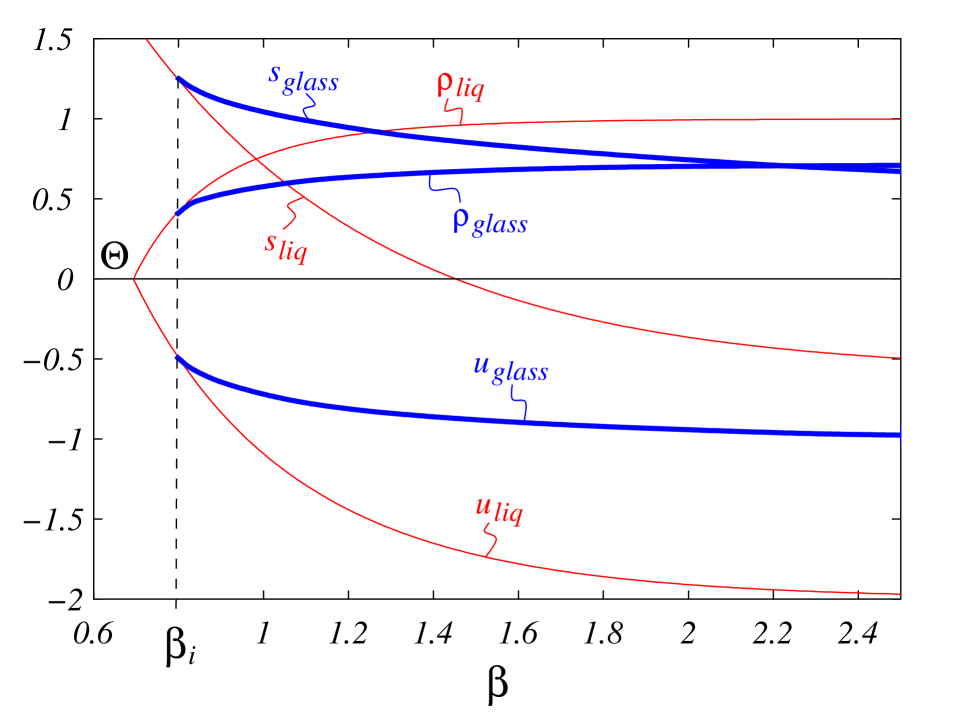
Figure 5: Alternating ampholyte on a lattice with 6 neighbors per site. The thick lines show the density $\rho$, entropy $s$ and internal energy $u$ computed in the glass phase using the 1RSB approximation. The thin lines give the corresponding values in the liquid solution, which is unstable beyond $\beta_{i}\approx 0.7947$. The glass transition is continuous.

In App. E we explain how to compute the order parameter (17) within the cavity approximation. The result for the alternating ampholyte is shown in Fig. 6, which again shows a continuous transition.

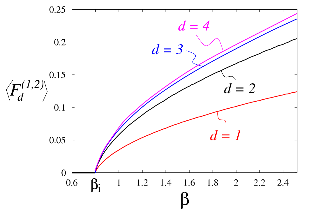
Figure 6: Alternating ampholyte: The order parameters $\left\langle F_{d}^{(1,2)}\right\rangle_{\rm state}$ for the glass phase, defined as the time persistent part of the distance vector between monomers at a distance $d=1,2,3,4$ in the backbone (see (17)), plotted versus the inverse temperature $\beta$.

V.3 The discontinuous transition in the alternating HP model

The case of the symmetrized-HP alternating sequence, always on a lattice with connectivity $k+1=6$, is extreme in the opposite sense. The liquid solution is always locally stable, even in the region of negative entropy. However, running the population dynamics algorithm for the 1RSB cavity method, one finds a discontinuous glass transition. The dynamic transition takes place at $\beta_{d}\approx 1.387$, just before the entropy crisis of the liquid ($\beta_{\rm cris}=1.4525$). The static phase transition follows at $\beta_{s}\approx 1.442$, in a region of very high density, $\rho\approx 0.95$, and almost vanishing entropy. In Fig. 7, we plot the density, entropy and internal energy for the alternating HP-polymer along the coexistence curve. The internal entropy of the statically dominating pure states is seen to nearly vanish in the frozen phase, and the system barely evolves upon lowering the temperature. This scenario is very similar to the abrupt freezing encountered in the random energy model (REM).

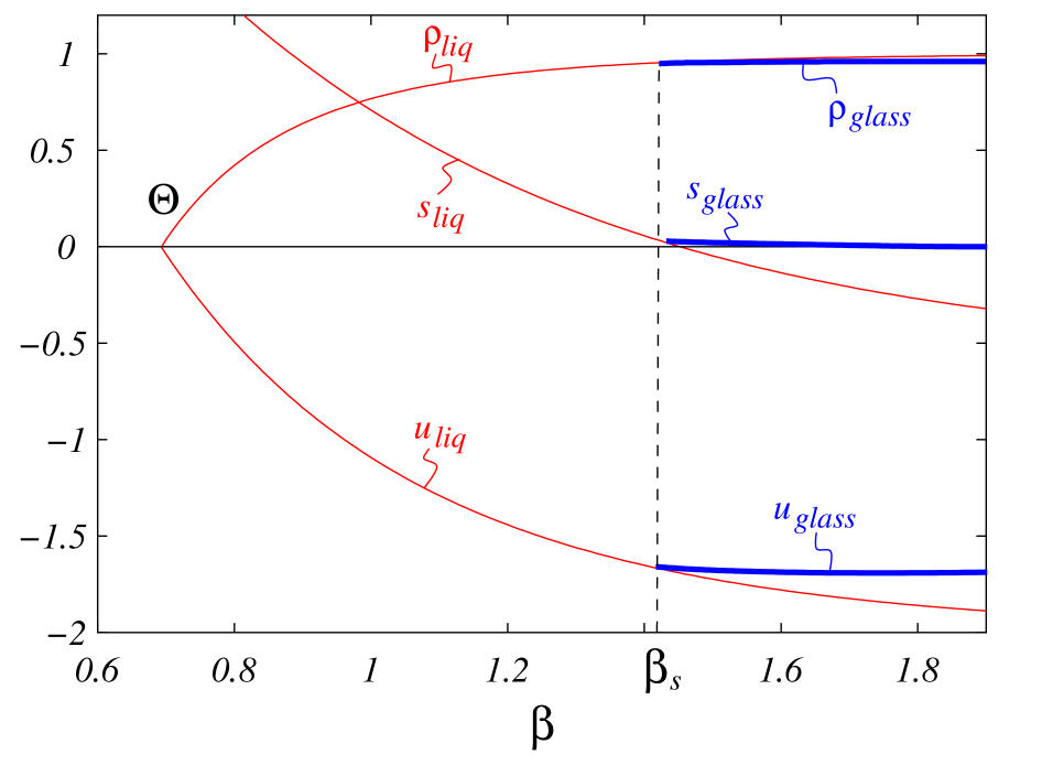
Figure 7: Alternating HP-like polymer on a lattice with 6 neighbors per site: The thick lines show the density $\rho$, entropy $s$ and internal energy $u$ computed in the glass phase using the 1RSB approximation. The thin lines give the corresponding values in the liquid solution, which is always locally stable. The glass transition is a discontinuous one; it is an almost perfect freezing transition as in the REM.

The computation of the order parameter (17) proceeds as in the case of the ampholyte. The result is shown in Fig. 8 and shows clearly the discontinuous transition.

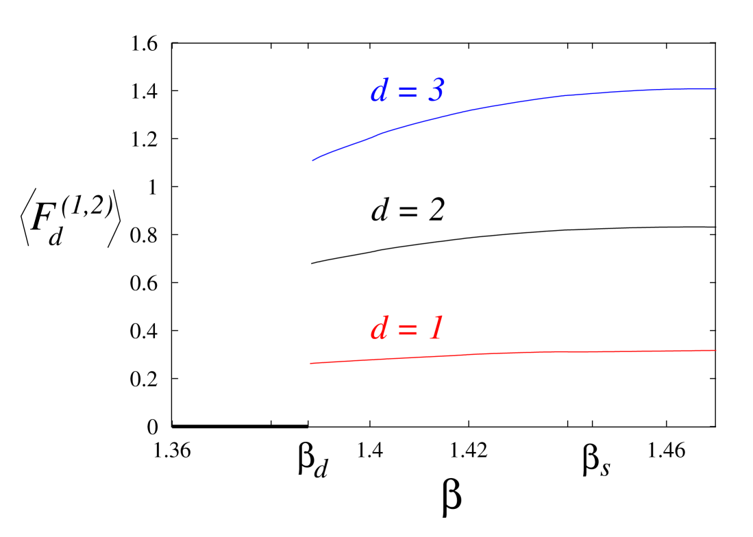
Figure 8: Alternating HP-like polymer: The structural order parameters $\left\langle F_{d}^{(1,2)}\right\rangle_{\rm state}$ for the glass phase, plotted versus the inverse temperature $\beta$. Note the considerably higher values than in Fig. 6, indicating a much stronger freezing of local conformational degrees of freedom.

V.4 Numerical simulations

As we already stressed, one advantage of our approach consists in the possibility of checking mean field computations using numerical simulations of well defined polymer models on a Bethe lattice. Here we want to demonstrate this feature by considering the alternating AB ampholyte.

Figure 9: Average length of the polymers simulated on the Bethe lattice. Sizes of the lattice are indicated in the legend. The arrow signal the liquid-soft glass phase transition.

We made extensive simulations on Bethe lattices with connectivity $(k+1)=6$ and volumes $V$ ranging from $100$ to $800$. For all of the data presented in this Section, we fixed $\beta=2.0$ above the $\Theta$-point inverse temperature $\beta_{\Theta}\approx 0.693$ and varied the chemical potential $\mu$. As $\mu$ is increased, the system undergoes at first a second order collapse transition (at $\mu\approx-3.21887$) and then a continuous glass transition to the soft-glass phase ($\mu_{i}(\beta)\approx-2.38431$).

Notice that most of the algorithms for simulating polymers on finite-dimensional graphs cannot be applied to the Bethe lattice. In fact local moves are impossible because of the absence of short loops. On the other hand, global moves would require a detailed knowledge of the loop structure for any graph realization.

This problem can be overcome by simulating a melt of variable-length polymers, the length being finite in the thermodynamic limit. The single-polymer physics is recovered when the average length diverges. We refer to App. F for a detailed description of our algorithm. In Fig. 9 we show our numerical data for the average polymer length $\left\langle l\right\rangle$. Notice that $\left\langle l\right\rangle\approx 10\div 25$ within the dense phase. As will be clear from the other numerical results, this is enough for assuring small deviations from the infinite-length limit. The main effects are: a rounding of the collapse transition and a small shift of the soft glass transition (which occurs at $\mu_{i}(\beta,\mbox{finite }l)\approx-2.40923$).

In order to achieve equilibration within the soft glass phase we adopted the parallel tempering technique Nemoto96 ; Marinari98 . We tested equilibration using the method of Ref. BhattYoung88 , and always checked the acceptance rate for temperature-exchange moves to be larger than $50\%$.

Figure 10: Simulations of the alternating ampholyte on the Bethe lattice with connectivity $k+1=6$. The energy per site of the polymer (left) and its density (right) are plotted versus the chemical potential. In the main frames numerical data (symbols) for various lattice sizes are compared with the cavity results (dashed line) for average polymer length $\left\langle l\right\rangle\to\infty$. The agreement is very good. In the insets we plot the liquid prediction for infinite (continuous line) and finite (dashed line) average polymer length, which shows that the finite length corrections are already small. Notice that in the density inset the finite-length theoretical curve is barely visible because it is superimposed on the data. The arrows indicate the analytic result for the glass transition point $\mu_{i}$.

In Fig. 10 we plot the energy per lattice site and the monomer density, as functions of the chemical potential $\mu$. Notice that the liquid - soft glass phase transition is barely discernible from the monomer density, and the energy curve is also quite smooth. The 1RSB cavity result gives a very good quantitative description of the transition.

Figure 11: Left: Finite-size scaling of the spin glass susceptibility, that exhibits a clear divergence as a function of system size at the expected value $\mu_{c}$. Right: probability distribution of the AB overlap, evaluated in the soft glass phase at $\mu=-1$. In the inset of the left frame we compare the second moment of the AB overlap $\overline{\left\langle q_{AB}^{2}\right\rangle}$ with the analytical prediction.

In order to get a finer description of the glass phase, we have measured the order parameter function $P_{AB}(q)$ defined in (20). In Fig. 11 we report our numerical data for this quantity at the highest chemical potential considered ($\mu=-1$). Because of the large finite-$V$ effects, it would be difficult to conclude from the numerics alone that the infinite-$V$ function is non-trivial. However, the data agree with the 1RSB predictions for the Edwards-Anderson parameter, $q_{\rm EA}\approx 0.259$.

In the same figure (left frame) we consider the spin-glass susceptibility:

$$\chi_{\rm SG}=\frac{1}{V}\sum_{i,j}\overline{\left\langle s_{i}s_{j}\right\rangle^{2}}=V\overline{\left\langle\left[q_{AB}(s^{(1)},s^{(2)})\right]^{2}\right\rangle}\,,$$ (27)

This quantity diverges as $\mu\to\mu_{c}^{-}$ in the thermodynamic limit. In a finite size sample, its behavior is ruled by the usual finite-size scaling form

$$\chi_{\rm SG}(V,\mu)=V^{2-\eta}\,\overline{\chi}[V^{1/\nu}(\mu-\mu_{c})]\,.$$ (28)

From the cavity solution of the model, one finds that $\overline{\left\langle q_{AB}^{2}\right\rangle}\approx A(\beta)[\mu-\mu_{c}(\beta)]^{2}$ for $\mu\gtrsim\mu_{c}(\beta)$. This result implies the following relation between the critical exponents defined in Eq. (28):

$$2-\eta+2/\nu=1\,.$$ (29)

In fact we find a nice collapse of data corresponding to different sizes using $\nu=4$ and $\eta=3/2$. The comparison of $\left\langle q_{AB}^{2}\right\rangle$ with the 1RSB cavity prediction is quite good.

Figure 12: Average AB overlap $\overline{\left\langle q_{AB}\right\rangle}$ among two replicas coupled through a term of the type $-N\epsilon q_{\rm AB}$. The full line is the prediction from the cavity method for the zero $\epsilon$ limit. Here $V=10^{4}$.

An alternative approach for exploring the low energy structure of the system consists in coupling two replicas through their overlap, cf. Eq. (19). In practice, one adds a term of the form $-N\beta\epsilon q_{AB}(s^{(1)},s^{(2)})$ to the two-replica Hamiltonian and tries to estimate $q_{\rm EA}$ as follows

$$q_{\rm EA}=\lim_{\epsilon\to 0}\lim_{N\to\infty}\overline{\left\langle q_{\rm AB}(s^{(1)},s^{(2)})\right\rangle_{N,\epsilon}}\,.$$ (30)

In Fig. 12 we show the numerical results for $\overline{\left\langle q_{\rm AB}\right\rangle_{N,\epsilon}}$ on a large size lattice ($V=10^{4}$) and several values of $\epsilon$. In order to simulate large lattices, we did not use parallel tempering here. Furthermore, we adopted a weaker equilibration criterium, requiring $\overline{\left\langle q_{\rm AB}\right\rangle_{N,\epsilon}}$ to be roughly time-independent on a logarithmic scale. Once again, the numerical results compare favorably with the outcome of the cavity calculation.

VI Random Markovian copolymers

One can show using the formula (23) that the local instability appears the earlier, the stronger the tendency of monomers to be annealed along the sequence, that is, the more $A$’s and $B$’s tend to alternate in an ampholyte, or to form blocks in an HP model. In both cases the autocorrelation function $q_{i}$ is large and its sign oscillates (alternating sequence) or remain positive (‘blocky’ sequence).

To be more quantitative, let us consider a random copolymer chain in the limit $L\rightarrow\infty$ characterized by the probability $\pi\in[0,1]$ of two neighboring monomers to be of the same type. The autocorrelation function of such a chain is (in the $L\to\infty$ limit) $q_{i}=(2\pi-1)^{i}$.

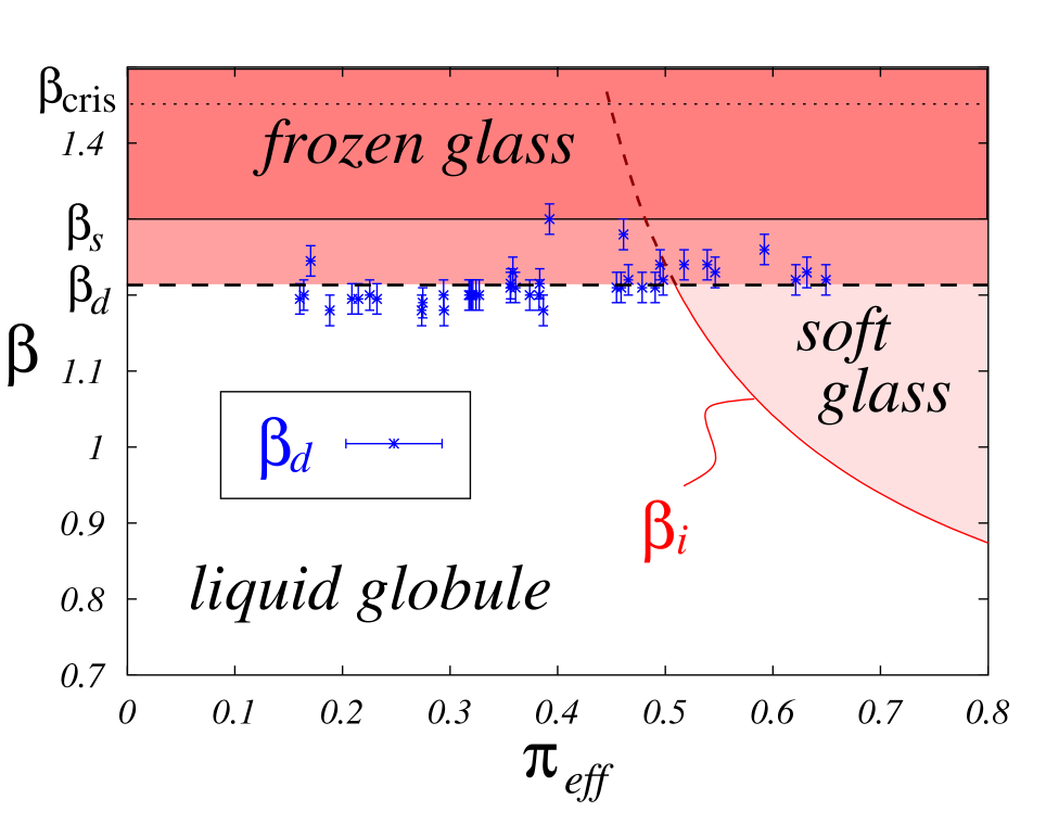
Figure 14: The same general phenomenology as in the ampholyte, cf. Fig. 13, holds for the HP-type models, but here, the continuous transition takes place at $\pi\geq 0.5$. Notice that the $\pi_{\rm eff}$ window displayed here is larger than in Fig. 13.

In Figs. 13 and 14 we plot the inverse temperature $\beta_{i}$ at the local instability as a function of the parameter $\pi$ for the ampholyte and symmetrized-HP models.

This instability is certainly irrelevant when $\beta_{i}$ is larger than the inverse temperature of the entropy crisis of the liquid, $\beta_{\rm cris}=1.4525$. This situation occurs for $\pi>0.4480$ in ampholytes, and proves the existence of a discontinuous transition. But already when $\beta_{i}$ is smaller than, but close to, $\beta_{\rm cris}$, one should expect a discontinuous 1RSB transition to take place at a $\beta<\beta_{i}$.

In order to complete the diagram, we have numerically solved the cavity recursion by population dynamics for neutral sequences of period $L=20$, but otherwise random composition. From the experience gained for the extreme case of the alternating HP-model (see below), we expected a kind of frozen solution with rather strong local conformational preferences to dominate the low temperature phase. Such a solution is rather non-trivial to find in a huge functional space, in particular since it has to be expected that it occurs in a discontinuous manner and cannot in general be found by randomly perturbing the liquid solution.

We therefore proceeded by initializing the population in a highly polarized state that we will discuss in more detail in the next Section. This state actually corresponds to an unstable fixed point, but it turns out that at low temperatures, it is usually quite close to a stable non-trivial solution of the 1RSB cavity equations. At each temperature, we iterated the cavity recursion for about 100 sweeps of the population dynamics, cf. App. G, fixing the chemical potential to its liquid critical value, since this value describes correctly the thermodynamic equilibrium up to the static phase transition. The Parisi reweighting parameter was set to $m=1$ in order to detect the dynamic transition, i.e., the local instability of the frozen solution. For reasons of numerical stability, we restricted ourselves to sequences with an anti-palindromic structure, i.e., sequences invariant under inversion and subsequent exchange of $A$’s and $B$’s. The field distributions $\rho({\bf p})$ inherit this invariance, and thus in each update of a new cavity field we can decide at random to apply a symmetry operation to the new fields first. This stabilizes the iteration since it counteracts the numerical tendency to spontaneously break the balance between $\uparrow$- and $\downarrow$-states. Indeed, there is a gauge degree of freedom associated to the relative weight of the two orientations of the chain, and in general it is difficult to maintain them balanced, while it can be enforced in sequences with a palindromic symmetry. The reason to choose antipalindromic rather than palindromic ones is to avoid at the same time an asymmetry between $A$- and $B$-states which likely occurs in small populations, in particular in the case of attractive interactions among equal monomers.

Our findings for the sequences of period $L=20$ are summarized in the plots 13, 14 and 15. Figure 15 shows the variance (square of the standard deviation) of the local field for $\uparrow(a=1)$ over the distribution $\rho({\bf p})$ for several sequences as a function of inverse temperature. This is a measure for the degree of the local bias away from the liquid. Almost independently of the particular sequence statistics we find that for $\beta>\beta_{d}\approx 1.23$ a strongly frozen phase (with very low internal entropy) exists with an associated dynamic transition at $\beta_{d}$. Depending on the sequence statistics, the regime of higher temperatures is either entirely liquid (e.g., for $\pi\leq 0.50$ in the ampholytes), or exhibits a weaker form of frustration in a phase of presumably fully broken replica symmetry. The latter continuously joins the liquid solution at the local instability predicted by (23). For the phase diagram in the $\beta-\mu$-plane for either of the two scenarios we refer to Figs. 3.

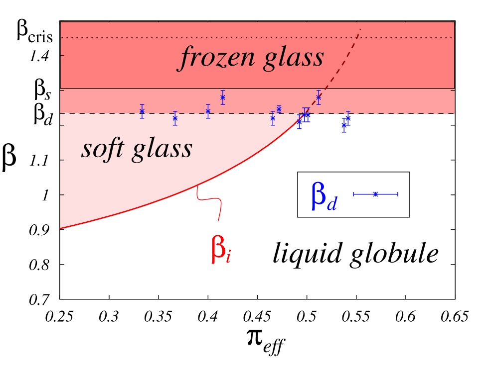
Figure 13: Phase diagram for ampholytes as a function of sequence correlations and inverse temperature. The continuous line indicates the local instability $\beta_{i}$ of the liquid as a function of the Markov chain parameter $\pi$. The points with error bars indicate the dynamic phase transitions $\beta_{d}$ found numerically for several sequences of period $L=20$ whereby we associated an effective parameter $\pi_{\rm eff}$ to each chain such that the local instability predicted from $\pi_{\rm eff}$ coincides with the actual one. Almost independently of the chain composition we find a highly frozen phase beyond $\beta_{d}\approx 1.23$ that is reached via a discontinuous glass transition well before the liquid would undergo an entropy crisis at $\beta_{\rm cris}$. For $\pi\leq 0.50$, this freezing is preceded by a continuous glass transition, as predicted from the local stability analysis of the liquid. The actual thermodynamic freezing transition occurs at a lower temperature $\beta_{s}>\beta_{d}$. The horizontal lines for the static and dynamic transitions are an educated guess for the location of these transitions in the limit $L\rightarrow\infty$.

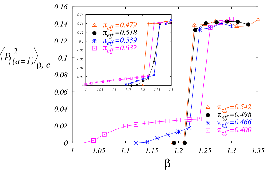
Figure 15: The variance $\left\langle p_{\uparrow(a=1)}^{2}\right\rangle_{\rho}-\left\langle p_{\uparrow(a=1)}\right\rangle_{\rho}^{2}$ of a selected local field as a function of inverse temperature for a variety of anti-palindromic sequences of period $L=20$. In general, there is a very distinct discontinuous transition around $\beta_{d}\approx 1.23$, that is preceded by a glassy regime with smaller fluctuations in the local fields if the sequence has a tendency for anticorrelation in ampholytes (main frame) or correlation in symmetrized HP-like chains (inset). The sequences are characterized by their effective Markov chain parameter $\pi_{\rm eff}$ as in Figs. 13 and 14.

The generic picture of a quench in temperature is thus the following: For ampholyte sequences with some tendency to alternation or HP-like-sequences with a preference for block formation, there is a continuous glass transition whose location depends strongly on the composition of the sequence. The corresponding glass phase is characterized by a relatively weak frustration and a rather small number of states that comprise many microconfigurations with some weak local preferences for certain conformations. This preliminary glass phase undergoes a further discontinuous phase transition at a lower temperature $\beta_{d}\approx 1.23$ that is almost independent of the sequence structure and might be called the effective freezing transition. For sequences with correlations of the opposite kind, the freezing transition is the only phase transition and occurs directly from the liquid. It is interesting to note that in numerical simulations of the folding dynamics of neutral HP-type copolymers, the dynamical glass transition was also found to be essentially independent of the sequence BryngelsonReview95 .

It is intriguing that the critical parameter of $\pi$ separating the FRSB from the 1RSB freezing scenario is very close to $\pi=1/2$ which corresponds to sequences without correlations. This is particularly interesting from the point of view of protein folding. The nature of correlations present in the amino acid sequences of natural proteins is still a matter of intensive debate. The analysis of Pande et al. PandeCorrelations argues in favor of a tendency for sequences to be annealed, i.e., to exhibit positive correlations in the hydrophilicity and anticorrelations in the charge of amino acids, which would suggest a bias towards the FRSB freezing scenario for proteins. However, the studies by Irbäck et al. Irbaeck96 ; Irbaeck97a ; Irbaeck97b rather point towards anticorrelations in the HP-type degrees of freedom which would favor a scenario with a direct transition from the liquid to the frozen glass. The discrepancies of these studies mainly concern the nature of long range correlations while on the level of nearest neighbor correlations, the protein sequences appear to be rather random, having $\pi\approx 1/2$ with respect to both charge and hydrophobic/hydrophilic degrees of freedom. It would be very interesting to understand whether the folding of natural proteins takes advantage from their sequences being very close to the critical border between the two scenarios. On the other hand, as mentioned earlier, most protein sequence design schemes tend to result in (partially) annealed monomer chains which are therefore likely to exhibit the intermediate soft glass phase.

VII The close-packed limit

In this section we provide a detailed analysis of the frozen phase in the limit of high density. We first show the existence of a special ‘REM-like’ fully polarized solution of the 1RSB cavity equations at temperatures below the liquid’s entropy crisis. Then we show that this solution is stable in the close-packed limit of high densities.

VII.1 A fully polarized solution

There always exists a ‘fully polarized’ solution to the cavity equation (24) which describes pure states consisting of essentially one unique frozen polymer configuration. In each such state, a given site only admits one specific local conformation. On averaging over the different pure states, the given site will be found in conformation $\alpha$ with frequency $w_{\alpha}$. The local field distributions then take the form

$$\rho_{\rm pol}({\bf p})=\sum_{\alpha}w_{\alpha}(\beta,m)\delta({\bf p}-{\bf e}^{(\alpha)}),$$ (31)

where the fields ${\bf e}^{(\alpha)}$ are defined by $e^{(\alpha)}_{\alpha^{\prime}}=\delta_{\alpha\alpha^{\prime}}$. This distribution solves the cavity equations when the frequencies $w_{\alpha}(\beta,m)$ coincide with the local fields of a liquid at the renormalized inverse temperature $\beta^{\prime}=m\beta$, i.e., $w_{\alpha}(\beta,m)=p^{*}_{\alpha}(\beta^{\prime}=m\beta)$. The replicated free energy of this fully polarized solution is $\phi_{1}(\beta,m)=\phi_{\rm liq}(m\beta)$. The internal free energy of the corresponding frozen states is related to the liquid quantities via $f_{\rm pol}(\beta,m)=d(m\phi_{1}(\beta,m))/dm=u_{\rm liq}(m\beta)-\mu\rho_{\rm liq}(m\beta)$, and the complexity of states is found from $\Sigma_{\rm pol}(\beta,m)=s_{\rm liq}(m\beta)$. As is evident from the nature of the pure states, their internal entropy vanishes.

Let us for a moment postpone the discussion of the relevance of this solution, and first discuss its physical interpretation. At each value of $\beta$ we have to maximize $\phi_{1}$ over $0\leq m\leq 1$, under the condition $\Sigma\geq 0$. For temperatures above the liquid’s entropy crisis, $\beta<\beta_{\rm cris}$, the maximum is attained at $m=1$ and we have $\omega_{g}=\omega_{\rm liq}$. When $\beta>\beta_{\rm cris}$, the static glass transition takes place and the free energy freezes to $\omega_{g}=\omega_{\rm liq}(\beta_{\rm cris})$, the Parisi parameter taking the value $m_{s}=\beta_{\rm cris}/\beta$. So this solution describes a full freezing of the polymer in some isolated specific configurations, taking place at $\beta=\beta_{\rm cris}$. Notice that this scenario exactly parallels the one found in the REM.

Our numerical study of the AB-copolymers in their highly frozen phase (beyond $\beta_{d}\approx 1.23$) finds a solution $\rho({\bf p})$ which is close to the form (31), although small deviations persist, and the polarization is not complete. In the particular case of the alternating chain we numerically confirmed that the optimal Parisi parameter is well fitted by $m_{s}=T/T_{s}$ on the coexistence line.

VII.2 Stability analysis and the limit of maximal density

Up to this point we have not discussed the range of validity of the polarized solution (31), and in particular, its stability. Unfortunately, this is a difficult problem, and we only can provide partial answers.

The basic idea consists in perturbing the Ansatz (31) and checking whether the perturbation grows under the cavity iteration (24). A simple perturbation consists in adding to (31) some ‘almost polarized’ fields with a small total weight. Namely we take a field distribution of the form

$$\rho({\bf p})=(1-a\varepsilon)\rho_{\rm pol}({\bf p})+\varepsilon\sum_{\alpha}w_{\alpha}\rho_{\alpha}({\bf p})\,,$$ (32)

where $\rho_{\alpha}({\bf p})$ is concentrated on fields ${\bf p}$ close to ${\bf e}^{(\alpha)}$. In fact, it is more convenient to think of it as a distribution over the ‘small’ fields $\vec{p}\equiv\{p_{\alpha^{\prime}}\}_{\alpha^{\prime}\neq\alpha}$. Hereafter, we shall use the notation $\rho_{\alpha}(\vec{p})$ instead of $\rho_{\alpha}({\bf p})$. Finally notice that the $\rho_{\alpha}(\vec{p})$’s need not to be normalized. Normalization is enforced by the constant $a$ in Eq. (32).

Plugging the nsatz (32) into Eq. (24) we get to linear order in $\epsilon$:

$$\rho^{\prime}_{\alpha_{0}}(\vec{p})=k\sum_{\alpha_{1}\dots\alpha_{k}}\!P(\alpha_{1}\dots\alpha_{k}|\alpha_{0})\int\!d\rho_{\alpha_{1}}(\vec{q})\;\;\delta\left(\vec{p}-\vec{I}[\vec{q};\alpha_{2}\dots\alpha_{k}]\right)\,.$$ (33)

Here we distinguished the distribution on the right-hand side, $\rho_{\alpha}(\cdot)$ from the one on the left-hand side $\rho_{\alpha}^{\prime}(\cdot)$. In fact we are interested in the stability of the iteration (24) and not just in its fixed point. Here $P(\alpha_{1}\dots\alpha_{k}|\alpha_{0})$ is the probability of finding conformations $\alpha_{1}\dots\alpha_{k}$ on the $k$ leaves of the branch in Fig. 1, constrained to the root being in conformation $\alpha_{0}$. This must be computed within the solution described by Eq. (31) and can explicitly be written in terms of the weights $w_{\alpha}(\beta,m)$. Finally $\vec{I}[\vec{q};\alpha_{2}\dots\alpha_{k}]$ denotes the ‘small’ components of the cavity iteration:

$(\vec{I}[\vec{q};\alpha_{2}\dots\alpha_{k}])_{\alpha}=I_{\alpha}[{\bf q},{\bf e}^{(\alpha_{2})}\dots{\bf e}^{(\alpha_{k})}]$ for $\alpha\neq\alpha_{0}$.

Instead of continuing in full generality, let us consider the example of an alternating F-model in the closed-packed limit with $E_{AA}=E_{BB}=-E_{AB}=-1$ (remember that in this case we found a discontinuous phase transition with a highly polarized low temperature phase, cf. Sec. V.3). Eqs. (33) reduce to

$$\rho^{\prime}_{1A}(\vec{p}) = \sum_{n=0}^{k-1}f_{n}\,\delta(p_{2A},p_{2B})\,\int\!\!d\rho_{1B}(\vec{q})\;\;\delta\left(p_{1B}-e^{-2\beta(k-1-2n)}q_{1A}\right)+$$

$$+g_{A}\delta(p_{1B},p_{2B})\,\int\!\!d\rho_{2A}(\vec{q})\;\delta(p_{2A}-e^{-\beta}q_{1B})+g_{B}\delta(p_{1B},p_{2B})\,\int\!\!d\rho_{2B}(\vec{q})\;\delta(p_{2A}-e^{\beta}q_{1B})\,,$$

$$\rho^{\prime}_{2A}(\vec{p}) = 2\delta(p_{1B},p_{2B})\,\int\!\!d\rho_{1B}(\vec{q})\;\delta\left(p_{1A}-e^{\beta}q_{2A}-e^{-\beta}q_{2B}\right)\,,$$ (35)

plus two equations obtained by interchanging $A$ and $B$. Here we used the shorthand $\delta(x,y)=\delta(x)\delta(y)$ and expanded $\vec{I}[\vec{q};\alpha_{2}\dots\alpha_{k}]$ in the delta functions to linear order in $q_{\alpha}$ for $\alpha\neq\alpha_{1}$. The weights $\{f_{n}\}$ and $g_{A/B}$ are given by

$$f_{n}=\frac{1}{(2\cosh\beta m)^{k-1}}\,{k-1\choose n}\,e^{-\beta m(k-1-2n)}\,,\;\;\;\;g_{A/B}=\frac{k-1}{1+e^{\pm 2\beta m}}\,.$$ (36)

A little thought shows that, after one iteration of Eqs. (VII.2), (35) we can set

$$\rho_{1A}(\vec{p}) = \delta(p_{2A},p_{2B})\;\rho_{1A\to 1B}(p_{1B})+\delta(p_{1B},p_{2B})\;\rho_{1A\to 2A}(p_{2A})\,,$$ (37)

$$\rho_{2A}(\vec{p}) = \delta(p_{1B},p_{2B})\;\rho_{2A\to 1A}(p_{1A})\,.$$ (38)

and that the linearized recursions decouple in the three ‘sectors’ $\{1A\to 1B,1B\to 1A\}$, $\{1A\to 2A,2B\to 1B\}$, $\{1B\to 2B,2A\to 1A\}$. The first sector corresponds to shifts of the chain and turns out to be marginally stable (the function $\vec{I}[\vec{q};\alpha_{2}\dots\alpha_{k}]$ has to be developed to second order in $\vec{q}$).

The other two sectors correspond to structural rearrangements of the backbone and become unstable when $m\beta<(m\beta)_{c}\equiv y_{c}=1/2\cdot\log(2k-3)$. This instability has a simple physical interpretation. The pure states described by $(m\beta)_{c}$ have a free energy density $f_{c}=1/2$. This means that on average, a randomly chosen site has one violated neighboring bond, i.e., one neighbor occupied by a monomer of the opposite type. It is thus possible to rearrange the backbone of the alternating chain without paying energy by opening the chain at the given site and redirecting it in the direction of the violated bond, and propagating the rearrangement through the lattice, see Fig. 16.

Figure 16: Instability of the completely frozen solution due to rearrangements of the backbone.

For $k\leq 6$ the instability appears at a smaller value than the liquid entropy crisis, $y_{c}<\beta_{\rm cris}(\mu\rightarrow\infty)$. Thus, at low temperatures, $\beta>y_{c}$, the thermodynamically relevant close packed states are correctly described by the stable polarized solution with $m_{s}=\beta_{\rm cris}/\beta$. In particular, we can immediately deduce the ground state energy of Hamiltonian walks of an alternating HP-chain on a fixed connectivity random graph from the value of $\phi_{\rm liq}(\beta_{\rm cris};\mu\rightarrow\infty)$: This yields $0.083686,0.120619,0.172602,0.236348$ violated bonds per site for $k=3,4,5$ and $6$, respectively.

A numerical study of the cavity recursion equations at maximal density actually finds, for $k\leq 6$, a coexistence of the polarized solution with another solution in some intermediate range $[y_{c},y_{t}]$. This is a peculiarity of the infinite $\mu$ regime, the numerics at finite but large $\mu$ suggesting that the polarized solution is unphysical below $y_{t}$. However, since $y_{t}<\beta_{\rm cris}$, the polarized Ansatz still correctly describes the low temperature regime.

What happens away from the $\mu\to\infty$ limit? The possibility of voids allows for new terms in the sum over conformations, cf. Eq. (33). It turns out that the iterations become unstable in the new sectors $\{0\to\uparrow a,\uparrow a\to 0\}$ and $\{0\to\downarrow a,\downarrow a\to 0\}$. Physically, this means that the presence of voids in the lattice always allows for a rearrangement of the polymer configuration in some (perhaps very rare) regions, preventing a complete freezing in a single state. Still, at $y\geq y_{t}$ a stable fixed point close to the polarized solution (31) exists.

Let us finally notice that the stability of the polarized solution can be studied within a larger 2RSB Ansatz MontanariRicci03 . The results coincide with the simplified treatment presented here. These results are further confirmed if one studies the behavior of field distributions in the $T\to 0$ limit following Ref. MontanariParisiRicci04 .

VII.3 Exact enumerations on a cube

In an attempt to verify the 1RSB or even REM-like nature of heteropolymers, Shakhnovich and Gutin have exactly enumerated all conformations of fully compact random 27-mers on a $3\times 3\times 3$ cube and calculated the overlap distribution function $P(q)$ as a function of temperature 27mer ; 27mer93 . They interpreted their results in favor of a REM-like scenario where only a small number of states dominated the low temperature regime and $P(q)$ exhibited typical features of a discontinuous glass phase. In view of our mean field predictions, one would expect to find a different scenario when repeating this analysis for copolymers (with a certain amount of sequence correlations) in their soft glass phase.

We first repeated this enumeration study for random ampholytes, and found a $P(q)$ order parameter very similar to the random bond case studied originally 27mer , in agreement with the results of 27mer93 . However the same analysis done for correlated ampholytic sequences with various values of $\pi$ did not show any clear dependence on $\pi$. This absence of evidence can have two origins. On the one hand it might be due to the extreme restrictions that full packing imposes on the conformations. We have seen above that the fully dense limit is very subtle since physically important degrees of freedom, which are found in a system with voids, are artificially suppressed, as has been put forward by many authors nonergodicpolymer ; Grosberg00 ; Timoshenko98 . On the other hand it seems that these sizes are too small to study the true phase space structure of the glass phase.

VIII Discussion and Conclusion

The cavity method approaches the lattice heteropolymer problem from a new point of view in that it analyzes the conformational degrees of freedom of chains with quenched-in sequences. Furthermore, this method allows to study the whole temperature range and describes the $\Theta-collapse$ and the low temperature physics within the same formalism. In this sense we believe it provides an interesting new perspective in the analytic studies of heteropolymer folding.

With this local approach we have studied the frustration effects on a given site of the lattice. We find that the decisive features determining the nature of the low temperature physics are the short-range correlations in the monomer sequence. Polymers whose monomer distribution along the chain tends to be annealed have a proclivity to undergo a continuous glass transition to a soft glass phase before the strong freezing transition takes place. In oppositely correlated sequences the freezing occurs directly from the liquid phase. A weakly polarized phase with broken ergodicity and a high sensitivity to the specific sequence, has also been observed in the extensive numerical analysis of the phase diagram for specific hydrophilic/hydrophobic chains Timoshenko98 , and the qualitative differences found between selected sequences indeed reflect the general tendencies that we predict from the cavity analysis of the slightly different but closely related HP-like model.

The temperature of the dynamic transition at which highly frozen pure states appear is almost independent of the correlations in the sequence as we found from the numerical solution of the 1RSB cavity equations. For the time being we do not have a deeper understanding of this finding, which is in accordance with numerical observations in the dynamics of copolymer folding. We hope to obtain better analytical insight into this phenomenon from a thorough analysis of the stability of the highly polarized low temperature states. This would probably also explain why the border between the 2RSB freezing scenario with an intermediate soft glass and the scenario of a direct transition liquid-frozen glass is so close to the Markov parameter $\pi=1/2$, corresponding to uncorrelated chains.

It would be interesting to verify the predictions for Markovian chains experimentally (preferably with ampholytes where the pair interactions are rather strong). In fact it is possible to fabricate Markovian copolymers from a random polymerization process, where $\pi$ can be controlled by changing the chemical parameters of the solution. Furthermore, it will be very interesting to review the studies of sequence correlations in natural proteins in the light of our findings.

The results of the cavity method are expected to be exact for polymers on random (Bethe) lattices, as is indeed corroborated by numerical simulations. However, on real space lattices the Bethe approximation neglects the correlations arising from small loops.

It would thus be very important to check the effect of sequence correlations through numerical simulations of polymers on a cubic lattice, using our mean field predictions as a guideline. One regime in which the small loops of the cubic lattice can yield a behavior which is qualitatively different from the present mean field analysis is the case where the polymer has a strong tendency to form local crumples, as it happens in block copolymers which undergo a microphase separation. In order to study such problems analytically, it would be interesting to improve the Bethe approximation by considering enlarged cavities that contain not only a single site but a small cluster of nearby sites. This actually amounts to a further step in the framework of the cluster variational method. For the homopolymeric case a first step in this direction has been carried out in Pretti02cactus .

Already on the level of the simplest copolymer model we found a surprisingly rich phase diagram as a function of temperature and sequence correlations. But clearly, the cavity method is amenable to a number of generalizations that allow to study more sophisticated models of biopolymers, including for instance backbone stiffness, orientational degrees of freedom, or additional structural constraints such as the saturation of monomer-monomer interactions, which are crucial, e.g., for the folding of RNA.

Appendix A Finding the liquid solution

In this Appendix we show how the translation invariant liquid solution can be found by solving a set of $|{\cal A}|+2$ equations (instead of $3L+1$ equations as it may appear from Eqs. (4)-(7)). First of all it is convenient to make a change of variables defining

$$w^{(i)}_{0}\equiv\sum_{a=1}^{L}\,\frac{p_{2a}^{(i)}}{p_{0}^{(i)}}\,,\;\;\;\;\;\;z^{(i)}_{\uparrow a}\equiv\frac{p^{(i)}_{\uparrow a}}{p^{(i)}_{0}}\,,\;\;\;\;\;\;z^{(i)}_{\downarrow a}\equiv\frac{p^{(i)}_{\downarrow a}}{p^{(i)}_{0}}\;\;\;\;\;\;w^{(i)}_{\sigma}\equiv\sum_{a=1}^{L}\,\frac{p_{2a}^{(i)}}{p_{0}^{(i)}}\exp(-\beta E_{\sigma,\sigma_{a}})\,.$$ (39)

It is easy to see that the cavity equations (4)-(7)), the free energy (13) and all the others observables, can be rewritten in terms of these $2L+|{\cal A}|+1$ variables. In using the new variables, when not specified, we shall assume that the index $\sigma$ belongs to the enlarged space $\{0\}\cup{\cal A}$. We will set $E_{0,\sigma}=E_{\sigma,0}=0$.

The liquid fixed point has the translation invariant form $w^{(i)}_{\sigma}=w_{\sigma}$, $z^{(i)}_{\uparrow a}=z_{\uparrow a}$, $z^{(i)}_{\downarrow a}=z_{\downarrow a}$. The corresponding equations are easily written:

$$z_{\uparrow a} = ke^{\beta\mu}\frac{z_{\uparrow,a+1}}{1+w_{0}}\,\left(\frac{1+w_{\sigma_{a}}}{1+w_{0}}\right)^{k-1}\,,$$ (40)

$$z_{\downarrow a} = ke^{\beta\mu}\frac{z_{\downarrow,a-1}}{1+w_{0}}\,\left(\frac{1+w_{\sigma_{a}}}{1+w_{0}}\right)^{k-1}\,,$$ (41)

$$w_{\sigma} = k(k-1)e^{\beta\mu}\sum_{a=1}^{L}\,e^{-\beta E_{\sigma,\sigma_{a}}}\frac{z_{\uparrow,a+1}}{1+w_{0}}\frac{z_{\downarrow,a-1}}{1+w_{0}}\left(\frac{1+w_{\sigma_{a}}}{1+w_{0}}\right)^{k-2}\,.$$ (42)

It is important to notice that the above equations are invariant under the transformation $z_{\uparrow a}\to\gamma\cdot z_{\uparrow a}$, $z_{\downarrow a}\to\gamma^{-1}\cdot z_{\downarrow a}$ for any positive $\gamma$: we shall fix this freedom below. The reader can easily check that any physical observable (such as the free energy, the local energy or the local density) is also invariant under such a transformation. This happens because, when following the chain along its conventional direction, each time we arrive at a site $i$, we are obliged to leave the site as well.

The above equations admit of course the trivial coil solution $z_{\uparrow a}=z_{\downarrow a}=0$. Moreover, if one has $z_{\uparrow a_{0}}=0$ ($z_{\downarrow a_{0}}=0$) for a particular $a_{0}$, this implies $z_{\uparrow a}=0$ ($z_{\downarrow a}=0$) for any $a$. Therefore, we shall hereafter assume that $z_{\uparrow a},z_{\downarrow a}\neq 0$ for any $a$. In this case Eqs. (40)-(41) imply the consistency condition

$$1=\left(\frac{ke^{\beta\mu}}{1+w_{0}}\right)^{L}\prod_{\sigma\in{\cal A}}\left(\frac{1+w_{\sigma}}{1+w_{0}}\right)^{(k-1)L\nu_{\sigma}}$$ (43)

Equations (40) and (41) are easily solved:

$$z_{\uparrow a} = \prod_{b=a}^{L}\frac{ke^{\beta\mu}}{1+w_{0}}\left(\frac{1+w_{\sigma_{b}}}{1+w_{0}}\right)^{k-1}\,z_{\uparrow}\,,$$ (44)

$$z_{\downarrow a} = \prod_{b=1}^{a}\frac{ke^{\beta\mu}}{1+w_{0}}\left(\frac{1+w_{\sigma_{b}}}{1+w_{0}}\right)^{k-1}\,z_{\downarrow}\,,$$ (45)

where $z_{\uparrow}$, $z_{\downarrow}$ are two integration constants. We can exploit the invariance mentioned above in order to fix $z_{\uparrow}=z_{\downarrow}=z$.

Plugging the expressions (44), (45) into Eq. (42), and using Eq. (43), we get

$$w_{\sigma}=(k-1)Lz^{2}\,\sum_{\tau\in{\cal A}}\frac{\nu_{\tau}e^{-\beta E_{\sigma\tau}}}{1+w_{\tau}}\,.$$ (46)

We are therefore left with a set of $|{\cal A}|+2$ equations (Eq. (43) plus the $|{\cal A}|+1$ equations in (46)) for $|{\cal A}|+2$ real variables ($z$ and the $|{\cal A}|+1$ variables $w_{\sigma}$). As anticipated these equations depend on the sequence just through the frequencies $\nu_{\sigma}$, $\sigma\in{\cal A}$. The reader will easily check that the same is true for any physical observable.

Near the $\Theta$ point all $w_{\sigma}$ are small, and (46) shows that to lowest order they satisfy $w_{\sigma}\approx w_{0}\sum_{\tau\in{\cal A}}\nu_{\tau}e^{-\beta E_{\sigma\tau}}$. By imposing that a non-trivial solution of (43) should exist one immediately obtains the equation (14) for the location of the $\Theta$ point.

Appendix B Neutral $AB$-copolymers: local stability analysis

Here we outline the computation of the local stability condition for an $AB$ copolymer having a generic period-$L$ sequence. We shall use, depending on the context, the two notations $\sigma_{a}\in\{A,B\}$, or $\sigma_{a}\in\{+,-\}$ for the sequence.

As already mentioned in Sec. IV.1, we consider the case of an interaction matrix symmetric under $A\leftrightarrow B$ interchange. Without loss of generality, we can restrict ourselves to the cases of the AF- and F-models defined in Sec. II.1. Moreover we shall assume that the sequence is neutral, i.e. $\nu_{A}=\nu_{B}=1/2$. Under these hypothesis, Eqs. (40)-(42) admit the symmetric solution $z_{\uparrow a}=z_{\downarrow a}=z/\sqrt{L}$, $w_{0}=w$, $w_{a}=w\cosh\beta$, where $z$ and $w$ are determined by solving the equations

$$z = ke^{\beta\mu}\left(\frac{z}{1+w}\right)\left(\frac{1+w\cosh\beta}{1+w}\right)^{k-1}\,,$$ (47)

$$w = k(k-1)e^{\beta\mu}\,\left(\frac{z}{1+w}\right)^{2}\left(\frac{1+w\cosh\beta}{1+w}\right)^{k-2}\,.$$ (48)

We want to compute the local stability of the cavity recursions (4)-(7) around the above solution. We therefore imagine that the cavity fields for one of the sites $1,\dots k$ (let us say the site $1$) have been slightly perturbed and compute the effect of such a perturbation on the site 0. To linear order we get:

$$\delta z^{(0)}_{\uparrow a} = A\,\delta z^{(1)}_{\uparrow,a+1}-B\,\delta w^{(1)}_{0}+C\,\delta w^{(1)}_{\sigma_{a}}\,,$$ (49)

$$\delta z^{(0)}_{\downarrow a} = A\,\delta z^{(1)}_{\downarrow,a-1}-B\,\delta w^{(1)}_{0}+C\,\delta w^{(1)}_{\sigma_{a}}\,,$$ (50)

$$\delta w^{(0)}_{0} = D\sum_{a=1}^{L}(\delta z^{(1)}_{\uparrow a}+\delta z^{(1)}_{\downarrow a})-E\,\delta w^{(1)}_{0}+F\,\sum_{\sigma\in\{A,B\}}\delta w^{(1)}_{\sigma}\,,$$ (51)

$$\delta w^{(0)}_{\sigma} = G\sum_{a=1}^{L}(e^{-\beta E_{\sigma\sigma(a-1)}}\delta z^{(1)}_{\uparrow,a}+e^{-\beta E_{\sigma\sigma(a+1)}}\delta z^{(1)}_{\downarrow,a})-H\,\delta w^{(1)}_{0}+F\,\sum_{\tau\in\{A,B\}}e^{-\beta E_{\sigma\tau}}\,\delta w^{(1)}_{\tau}\,.$$ (52)

The constants $A$–$H$ are all positive, and can be expressed in terms of the solution of Eqs. (47)-(48). In the following we will just need the combinations below:

$$A=\frac{1}{k}\,,\;\;\;\;\;\;\;\;CG=\frac{k-1}{k^{2}L}\frac{w}{1+cw}\,,\;\;\;\;\;\;\;\;F=\frac{k-2}{2k}\frac{w}{1+cw}\,,$$ (53)

where we used the shorthand $c\equiv\cosh\beta$.

We must now identify the most relevant perturbation, i.e., the largest eigenvalue of the linear transformation (49)-(52). It is simple to show that the subspace

$$\left\{\delta w_{0}=0;\;\sum_{a=1}^{L}\delta z_{\uparrow a}=0;\;\sum_{a=1}^{L}\delta z_{\downarrow a}=0;\;\sum_{\sigma\in\{A,B\}}\;\delta w_{\sigma}=0\right\}$$ (54)

is preserved by the iteration (49)-(52). It can be shown that the most relevant eigenvector lies indeed within this subspace. We restrict to it by defining the variables

$$\delta\overline{w}\equiv\delta w_{A}-\delta w_{B}\,,\;\;\;\;\;\delta_{\uparrow b}\equiv\sum_{a=1}^{L}\delta z_{\uparrow a}\,\sigma_{a-b}\,\;\;\;\;\delta_{\downarrow b}\equiv\sum_{a=1}^{L}\delta z_{\downarrow a}\,\sigma_{a+b}\,,$$ (55)

where we used $\sigma_{a}\in\{+,-\}$ for the polymer sequence. Using the new variables we can rewrite the iteration (49)-(52) as follows:

$$\delta^{(0)}_{\uparrow a} = A\,\delta^{(1)}_{\uparrow,a+1}+\frac{L}{2}Cq_{-a}\,\delta\overline{w}^{(1)}\,,$$ (56)

$$\delta^{(0)}_{\downarrow a} = A\,\delta^{(1)}_{\downarrow,a+1}+\frac{L}{2}Cq_{a}\,\delta\overline{w}^{(1)}\,,$$ (57)

$$\delta\overline{w}^{(0)} = 2Gs\,(\delta^{(1)}_{\uparrow 1}+\delta^{(1)}_{\downarrow 1})+2Fs\,\delta\overline{w}^{(1)}\,,$$ (58)

where we introduced the notation $s\equiv\sinh\beta$ (for the F-model) or $s\equiv-\sinh\beta$ (for the AF-model), and the sequence correlation function

$$q_{b}=\frac{1}{L}\sum_{a=1}^{L}\,\sigma_{a}\sigma_{a+b}\,.$$ (59)

Notice that $q_{b}=q_{-b}$. This remark allows us to sum Eqs. (56) and (57) and to introduce the Fourier transform (for $p=2\pi n/L$, $n\in\{1,\dots,L-1\}$):

$$\delta(p)=\sum_{a=1}^{L}\,(\delta_{\uparrow,a}+\delta_{\downarrow,a})\,e^{-ipa}\,.$$ (60)

We obtain therefore

$$\delta^{(0)}(p) = Ae^{ip}\,\delta^{(1)}(p)+LCq(p)\,\delta\overline{w}^{(1)}\,,$$ (61)

$$\delta\overline{w}^{(0)} = 2Gs\,\frac{1}{L}\sum_{p}\delta^{(1)}(p)\,e^{ip}+2Fs\,\delta\overline{w}^{(1)}\,.$$ (62)

We can now set $\delta^{(0)}(p)=\lambda\delta^{(1)}(p)$, $\delta\overline{w}^{(0)}=\lambda\delta\overline{w}^{(1)}$, and solve for $\lambda$, thus recovering Eq. (23).

Appendix C Coexistence condition for a many states molecule

It may be interesting to explicitly treat the case of an isolated molecule in equilibrium with the solvent and determine the coexistence condition in the glass phase. The result is not obvious since the system can exist in many different states $\gamma\in\{1,\dots{\cal N}\}$ with (extensive) grand potential $\{\Omega_{1},\dots,\Omega_{\cal N}\}$. Each one of these states describes a molecule confined to a volume $V$.

Let us suppose that each state can be traced as the volume $V$ of the system is changed. This gives us the volume-dependent potentials $\Omega_{\gamma}(V)$. If the state $\gamma$ is to describe a molecule in equilibrium with the solvent it should exert no pressure on the walls of the container:

$$\frac{d\Omega_{\gamma}}{dV}=0\,.$$ (63)

We want to compute the typical value of the above quantity for states having a certain free-energy density: $\Omega_{\gamma}\approx V\omega$. Let us step back for a moment and consider the extensive complexity $\widehat{\Sigma}(\Omega;V,\mu)$, where we made explicit the dependence upon the volume $V$ and the chemical potential $\mu$. If we assume that states do not bifurcate and do not die (or come into existence) as the volume is changed, it is easy to show that LopatinIoffe02 , for almost any state $\gamma$:

$$\widehat{\Sigma}(\Omega_{\gamma}+d\Omega_{\gamma};V+dV,\mu)=\widehat{\Sigma}(\Omega_{\gamma};V,\mu)\,.$$ (64)

Using the asymptotic behavior $\widehat{\Sigma}(\Omega;V,\mu)\approx V\Sigma(\omega,\mu)$, and the general relations from Sec. III.1 we can establish the coexistence condition either in the $(m,\mu)$ or in the $(\omega,\mu)$ plane (we always assume $\beta$ and the energy parameters to be fixed). From (64), we immediately obtain the condition in the $(\mu,\omega)$ plane:

$$\omega\frac{\partial\Sigma}{\partial\omega}(\omega,\mu)=\Sigma(\omega,\mu)\,.$$ (65)

This is suggestive of a balance between an “internal” osmotic pressure, $\omega$, and an “interstate” pressure ($\Sigma/\partial_{\omega}\Sigma$). In the $(m,\mu)$ plane, the condition assumes a more compact form $\phi_{1}(m,\mu)=0$. If we consider the lowest lying states, their free energy density $\omega_{\rm s}(\mu)$ is determined by the vanishing of the complexity: $\Sigma(\omega_{\rm s}(\mu),\mu)=0$. Therefore Eq. (65) is satisfied for $\mu=\mu_{\rm s}$, with $\omega_{\rm s}(\mu_{\rm s})=0$. This coincides with the condition for a unique pure state. If metastable states are considered, Eq. (65) receives a non-vanishing contribution from the complexity: in particular, one obtains $\omega>0$. This is quite striking since we did not assume the system to equilibrate among states of a given free-energy (which indeed does not happen on the short time scales that are relevant to determine the boundary conditions with the solvent).

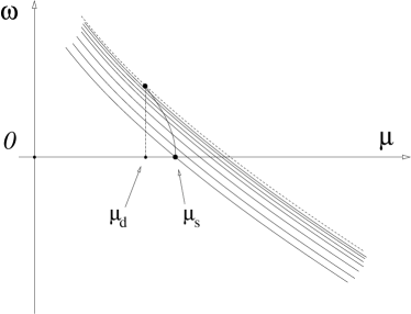
Figure 17: A schematic view of the coexistence between a multi-state molecule and the solvent. Each line represents the evolution of the internal free energy of a state as the volume is changed ($\Sigma(\omega,\mu)=const.$). The thick line shows the states which are in equilibrium with the solvent. In particular, we signal the coexistence chemical potentials for static and dynamic states.

In Fig. 17 we represent the condition (65) in the $(\omega,\mu)$ plane. Notice that in general metastable states (with $\Sigma>0$) on the coexistence line correspond to lower chemical potential than that of thermodynamically relevant states.

Let us finally consider the coexistence line at thermodynamic equilibrium. Dominant states are obtained by minimizing the free energy $\omega-\beta^{-1}\Sigma(\omega,\mu)$ with respect to $\omega$. The coexistence chemical potential $\mu_{*}$ is then obtained from Eq. (65). In a more compact (but formal) way, it is determined from the condition

$$\max\{\phi_{1}(m,\mu_{*})|m\in[0,1]\}=0\,.$$ (66)

In the main body of the paper we focus on the behavior of the polymer on this line. Generally speaking, at high temperature the maximum in Eq. (66) is attained at $m=1$. Since $\phi_{1}(m=1,\mu)=\phi_{\rm liq}(\mu)$, in this region the coexistence line is the same as for the liquid phase. At lower temperatures the maximum is attained for $0<m_{*}<1$ and the thermodynamic coexistence line lies above the liquid one. We refer to Fig. 3 for a summary of this behavior.

Appendix D Expansion of moments at the continuous glass transition

Here we analyze the solution of the cavity recursion near the continuous transition to first non-trivial order in an expansion of its moments.

Using both sides of the cavity recursion equation on the 1RSB level (24) in order to calculate the moments of the cavity fields, one obtains a set of coupled non-linear equations for the moments of the fields $p_{\alpha}$ over the distribution $\rho({\bf p})$. It is convenient to change coordinates and define the fields $\Delta_{\mu}=\sum_{\alpha}A_{\mu}^{\,\alpha}(p_{\alpha}-p^{*}_{\alpha})$ in such a way as to diagonalize the matrix (22). Hereafter we shall denote by $\mu=1$ the most instable (‘replicon’) direction in this matrix, and by $\lambda$ the corresponding eigenvalue.

A careful analysis allows to establish the scaling of the moments with respect to the small parameter $k\lambda^{2}-1\sim T_{i}-T$ close to the instability (21). The leading moment is given by the second moment of the replicon mode. One finds $\left\langle\Delta_{1}^{2}\right\rangle\sim(T_{i}-T)$ (the brackets $\left\langle\right\rangle$ denote the average with respect to $\rho$), while all other moments of deviations from the liquid fixed point ${\bf p}^{*}$ are at least of second order in $T_{i}-T$. The only moments of order $(T_{i}-T)^{2}$ are the first order moments of $\left\langle\Delta_{\mu}\right\rangle$, the remaining second moments $\left\langle\Delta_{1}\Delta_{a}\right\rangle$, $\left\langle\Delta_{\mu}\Delta_{\nu}\right\rangle$, with $\mu,\nu>1$ and the higher moments $\left\langle\Delta_{1}^{3}\right\rangle$, $\left\langle\Delta_{1}^{2}\Delta_{\mu}\right\rangle$ and $\left\langle\Delta_{1}^{4}\right\rangle$.

We will exploit the knowledge about this scaling in order to expand the 1RSB free energy (25) in powers of $T_{i}-T$ around the liquid solution.

The site term gives rise to a series

$$\log\left[\left(w_{s}^{\rm liq}\right)^{m}\left(1+\left(\begin{array}[]{c}m\\ 1\end{array}\right)\left\langle\sum_{i=1}^{k+1}w_{s,\mu}\Delta^{(i)}_{\mu}+\frac{1}{2}\sum_{i\neq j}^{k+1}w_{s,\mu\nu}\Delta^{(i)}_{\mu}\Delta^{(j)}_{\nu}+\frac{1}{6}\sum_{i\neq j\neq l}^{k+1}w_{s,\mu\nu\rho}\Delta^{(i)}_{\mu}\Delta^{(j)}_{\nu}\Delta^{(l)}_{\rho}\dots\right\rangle\right.\right.$$ (69)

$$\left.\left.+\left(\begin{array}[]{c}m\\ 2\end{array}\right)\left\langle\left(\sum_{i=1}^{k+1}w_{s,\mu}\Delta^{(i)}_{\mu}+\frac{1}{2}\sum_{i\neq j}^{k+1}w_{s,\mu\nu}\Delta^{(i)}_{\mu}\Delta^{(j)}_{\nu}+\frac{1}{6}\sum_{i\neq j\neq l}^{k+1}w_{s,\mu\nu\rho}\Delta^{(i)}_{\mu}\Delta^{(j)}_{\nu}\Delta^{(l)}_{\rho}\dots\right)^{2}\right\rangle+\dots\right)\right]\,,$$ (72)

(73)

where summation over direction indices $\mu,\nu,\rho=1,\dots,3L$ is tacitly understood and we used the shorthand notation

$$w_{s,\mu}=\left[\frac{1}{w_{s}}\frac{\partial w_{s}}{\partial\Delta^{(1)}_{\mu}}\right]_{\rm liq},$$ (74)

$$w_{s,\mu\nu}=\left[\frac{1}{w_{s}}\frac{\partial^{2}w_{s}}{\partial\Delta^{(1)}_{\mu}\partial\Delta^{(2)}_{\nu}}\right]_{\rm liq},$$ (75)

$$w_{s,\mu\nu\rho}=\left[\frac{1}{w_{s}}\frac{\partial^{3}w_{s}}{\partial\Delta^{(1)}_{\mu}\partial\Delta^{(2)}_{\nu}\partial\Delta^{(3)}_{\rho}}\right]_{\rm liq}\,.$$ (76)

Note that we have made use of the fact that $w_{s}$ is a multi-linear function of the fields ${\bf p}^{(i)}$ so that higher derivatives have to occur with respect to variables on different sites. The average $\left\langle\right\rangle$ is with respect to the distributions $\rho({\bf p}^{(1)}),\dots,\rho({\bf p}^{(k+1)})$ on all sites. The link term has an analogous expansion as (73), but the triple sum vanishes since there are only two different field variables.

To proceed, we note the identity

$$w_{s}({\bf p}^{(1)},\dots,{\bf p}^{(k+1)})=C[{\bf p}^{(2)},\dots,{\bf p}^{(k+1)}]w_{l}({\bf p}^{(1)},I[{\bf p}^{(2)},\dots,{\bf p}^{(k+1)}]),$$ (77)

from which one immediately deduces

$$w_{s,\mu}=w_{l,\mu}$$ (78)

for all directions $\mu$. Using that $\partial C/\partial\Delta^{(2)}_{1}|_{\rm liq}=0$, as follows from the properties of the subspace (54) which the replicon belongs to, one further finds

$$w_{s,1}=w_{l,1}=0$$ (79)

and

$$w_{s,1\nu}=\lambda w_{l,1\nu}\,.$$ (80)

Let us now discuss the terms that appear to increasing order in $T_{i}-T$ in the expansion of the free energy. There is no first order term proportional to $\left\langle\Delta_{1}^{2}\right\rangle$, because of (79). The second order terms $\left\langle\Delta_{\mu}\right\rangle$, $\left\langle\Delta_{\mu}\Delta_{\nu}\right\rangle$, $\left\langle\Delta_{1}^{3}\right\rangle$, and $\left\langle\Delta_{1}^{2}\Delta_{\mu}\right\rangle$ come with products of factors $w_{s/l,\mu}$ and cancel exactly between the site and link contributions, due to (78). The only remaining term to second order is

$$\beta m\,\phi^{(2)}=\left(\begin{array}[]{c}m\\ 2\end{array}\right)\left[-\frac{(k+1)k}{2}\left(w_{s,11}\right)^{2}+\frac{k+1}{2}\left(w_{l,11}\right)^{2}\right]\left\langle\Delta_{1}^{2}\right\rangle^{2}.$$ (81)

However, using (80), the coefficient in brackets is seen to be of order $k\lambda^{2}-1\sim T_{i}-T$.

The same mechanism suppresses the a priori third order terms $\left\langle\Delta_{1}^{2}\right\rangle\left\langle\Delta_{\mu}\Delta_{\nu}\right\rangle$ and $\left\langle\Delta_{1}^{2}\right\rangle\left\langle\Delta_{1}^{2}\Delta_{\nu}\right\rangle$ by an additional factor $k\lambda^{2}-1$ while the terms $\left\langle\Delta_{1}^{2}\right\rangle\left\langle\Delta_{\mu}\right\rangle$, $\left\langle\Delta_{1}^{3}\right\rangle\left\langle\Delta_{1}^{2}\right\rangle$ and $\left\langle\Delta_{1}^{4}\right\rangle\left\langle\Delta_{1}^{2}\right\rangle$ do not appear, again because of (79). The only surviving third order contributions are the site terms proportional to $\left\langle\Delta_{1}^{2}\right\rangle^{3}$,

$$\beta m\,\phi^{(3)}=-(k+1)k(k-1)\left[\frac{1}{6}{m\choose 2}w_{s,111}^{2}+{m\choose 3}w_{s,11}^{3}\right]\left\langle\Delta_{1}^{2}\right\rangle^{3}.$$ (82)

To first non trivial order we finally have

$$\phi_{1} = \phi_{\rm liq}+\phi^{(2)}+\phi^{(3)}+O((k\lambda^{2}-1)^{4})$$

$$= \phi_{\rm liq}+\frac{1-m}{4\beta}(k+1)k\,w_{s,11}^{2}({k\lambda^{2}}-1)\left\langle\Delta_{1}^{2}\right\rangle^{2}$$

$$+\frac{1-m}{2\beta}(k+1)k(k-1)\left(\frac{1}{6}w_{s,111}^{2}-\frac{2-m}{3}w_{s,11}^{3}\right)\left\langle\Delta_{1}^{2}\right\rangle^{3}+O((k\lambda^{2}-1)^{4}).$$

Since the form (25) of the free energy is variational, we may obtain the leading moment to first order in $T_{i}-T$ from the condition $\partial\phi_{1}/\partial\left\langle\Delta_{1}^{2}\right\rangle=0$,

$$\left\langle\Delta_{1}^{2}\right\rangle=\frac{1}{(k-1)}\,\frac{w_{s,11}^{2}}{\left[(2-m)w_{s,11}^{3}-w_{s,111}^{2}/2\right]}(k\lambda^{2}-1)+O\left((k\lambda^{2}-1)^{2}\right)\,.$$ (84)

Plugging this result in Eq. (D) we get

$$\phi_{1} = \phi_{\rm liq}+\frac{(1-m)}{12\beta}\,\frac{k(k+1)}{(k-1)^{2}}\,\frac{w_{s,11}^{6}}{\left[(2-m)w_{s,11}^{3}-w_{s,111}^{2}/2\right]^{2}}\,(k\lambda^{2}-1)^{3}+O((k\lambda^{2}-1)^{4})\,.$$ (85)

Note that the prefactor of $(k\lambda^{2}-1)$ in Eq. (84) has to be positive for consistency. A negative value indicates that there is no stable solution close to the liquid fixed point and the glass transition would be discontinuous. By explicit calculation of this coefficient at the instability point we found this to happen only in very atypical sequences with highly non-symmetric interactions.

Evaluating the coefficients $w_{s,11}$ and $w_{s,111}$ requires the knowledge of the replicon eigenvector. This can be derived for the case of copolymers with symmetric interaction matrix $E_{AA}=E_{BB}=-E_{AB}$, and equally frequent monomer species, $\nu_{A}=\nu_{B}=1/2$, extending the arguments of App. B. In particular we obtain (using the variables defined in Apps. A and B):

$$\delta w_{0}=0\,,\;\;\;\delta z_{\uparrow a}=\frac{C\delta w}{2\lambda}\sum_{n=0}^{\infty}\sigma_{a+n}(k\lambda)^{-n}\,,\;\;\;\delta z_{\downarrow a}=\frac{C\delta w}{2\lambda}\sum_{n=0}^{\infty}\sigma_{a-n}(k\lambda)^{-n}\,,\;\;\;\delta w_{\sigma}=\sigma\delta w\,.$$ (86)

Things simplify considerably in several important cases: $(i)$ alternating copolymers; $(ii)$ anti-palindromic sequences; $(iii)$ Markov sequences in the $L\to\infty$ limit. In all this cases the ratio $w_{s,111}^{2}/w_{s,11}^{3}$ vanishes. The basic reason is that, because of Eq. (86), $w_{s,111}$ turns out to be an odd function of $\{\sigma_{a}\}$. In these cases the free energy $\phi_{1}(m)$ takes the simpler form, cf. (26),

$$\phi_{1}-\phi_{\rm liq}=\frac{(k+1)k^{2}}{12(k-1)^{2}\beta}\frac{1-m}{(2-m)^{2}}(k\lambda^{2}-1)^{3}+O\left((k\lambda^{2}-1)^{4}\right).$$ (87)

At the glass transition the maximum of $\phi_{1}$ is attained at $m_{s}=0$. The fourth order term will shift its position to $m_{s}\propto k\lambda^{2}-1\sim T_{i}-T$, as we have explicitly checked in the alternating AB-ampholyte.

Appendix E Computing the order parameter in the cavity method

We show here how to compute the local structural order parameters (17) using the cavity method.

In the spirit of the Bethe-Peierls approximation we treat the self-avoidance of the polymer chain just on a local level, forbidding it to leave a site on the edge on which it arrived, but neglecting further constraints that arise on a real space lattice. In the following, we call “non reversal random walks” (NRRW) this restricted class of walks on the cubic lattice.

Let us rewrite the distance vector between monomers $i$ and $i+d$ as $\vec{R}^{(1)}_{i+d}-\vec{R}^{(1)}_{i}=\sum_{n=1}^{d}\vec{r}^{(1)}_{n}$ with $\vec{r}^{(1)}_{n}=\vec{R}^{(1)}_{i+n}-\vec{R}^{(1)}_{i+n-1}$. If the positions along the chain are statistically equivalent, the overlap $\left\langle F_{d}\right\rangle_{\rm state}$ can be written as

$$\left\langle F_{d}^{(1,2)}\right\rangle_{\rm state}=\left\langle\sum_{l=0}^{d}\left(\sum_{n=1}^{l}\vec{r}_{n}+\sum_{n=l+1}^{d}\vec{r}^{(1)}_{n}\right)\cdot\left(\sum_{n=1}^{l}\vec{r}_{n}+\sum_{n=l+1}^{d}\vec{r}^{(2)}_{n}\right)\right\rangle_{\rm state}$$ (88)

where we split the sum according to the length $l$ over which the replicas stay together and put $\vec{r}_{n}^{(1)}=\vec{r}_{n}^{(2)}=\vec{r}_{n}$ for $n\leq l$. Note that once $l$ is fixed the common part of the path and the two legs of length $d-l$ can be considered as non reversal random walks, only subject to the constraint that the legs leave in different directions at the bifurcation. These random walks have all the same weight when averaging over pure states. Hence, in order to evaluate (88) it is sufficient to calculate the probability $\left\langle P(l)\right\rangle_{\rm state}$ for two replicas in the same state to follow the same path over a distance $l$, from which we obtain

$$\left\langle F_{d}^{(1,2)}\right\rangle_{\rm state}=\sum_{l=0}^{d}\left\langle P(l)\right\rangle_{\rm state}f(l;d)$$ (89)

where

$$f(l;d)=\left\langle\left(\sum_{n=1}^{l}\vec{r}_{n}+\sum_{n=l+1}^{d}\vec{r}^{(1)}_{n}\right)\cdot\left(\sum_{n=1}^{l}\vec{r}_{n}+\sum_{n=l+1}^{d}\vec{r}^{(2)}_{n}\right)\right\rangle_{NRRW(l)}\,,$$ (90)

the average being taken over the uniform distribution of two NRRW’s after $l$ common links.

Using that in a NRRW one has $\left\langle\vec{r}_{n_{1}}\cdot\vec{r}_{n_{2}}\right\rangle_{NRRW}=1/k^{|n_{1}-n_{2}|}$, and distinguishing the different possible conformations at the bifurcation, one easily finds

$$f(l;d)=l+2\sum_{j=1}^{l-1}\frac{l-j}{k^{j}}+\frac{2}{k}\sum_{n_{1}=1}^{l}\sum_{n_{2}=1}^{d-l}\frac{1}{k^{n_{1}+n_{2}-2}}-\frac{1}{k}\sum_{n_{1}=1}^{d-l}\sum_{n_{2}=1}^{d-l}\frac{1}{k^{n_{1}+n_{2}-2}}.$$ (91)

(The first two terms stem from the self overlap of the common part, the term in the middle is the cross term between the common part and a leg that continues straight with respect to the common part, and the last term is a negative contribution due to two legs leaving in opposite directions.)

In the liquid state, $\left\langle P(l)\right\rangle_{\rm liq}$ is just given by the probability that two NRRW’s stay together over a distance $l$,

$$P_{\rm liq}(l=0) = \frac{k}{k+1},$$ (92)

$$P_{\rm liq}(l>0) = \frac{k-1}{k+1}\frac{1}{k^{l}}.$$ (93)

Upon injecting (91), (92), and (93) in (89) one may verify that $\left\langle F_{d}\right\rangle_{\rm liq}=0$.

In the glass phase, $\left\langle P(l)\right\rangle_{\rm state}$ is most easily evaluated as $N(l)\left\langle\tilde{P}(l)\right\rangle_{\rm state}$, where $N(l)$ is the number of rooted NRRW’s of length $l$ and $\tilde{P}(l)$ is the probability for two replicas to stay on a specific path of length $l$.

In the Bethe-Peierls approximation the latter can be computed within an enlarged cavity containing all sites of the path. The average over the states is done by averaging independently over the local field distributions on all neighboring sites, taking into account proper weighting factors:

$$\left\langle\tilde{P}(l)\right\rangle_{\rm state}=\frac{1}{L}\sum_{a=1}^{L}\frac{\int\!\prod_{\iota\in\mathcal{I}_{l}}d\rho\left({\bf p}^{(\iota)}\right)\mathcal{P}_{l;a}\,W_{l;{\rm tot}}(\{{\bf p}^{\iota}\}_{\iota\in\mathcal{I}_{l}})^{m}}{\int\!\prod_{\iota\in\mathcal{I}_{l}}d\rho\left({\bf p}^{(\iota)}\right)W_{l;{\rm tot}}(\{{\bf p}^{\iota}\}_{\iota\in\mathcal{I}_{l}})^{m}}\,,$$ (94)

where we have introduced the set of indices $\mathcal{I}_{l}$ labeling the neighbors of the $l+1$ sites on the path:

$$\mathcal{I}_{l}=\cup_{i_{0}=1}^{k}\{(0,i_{0})\}\cup_{l^{\prime}=1}^{l-1}\left(\cup_{i_{l^{\prime}}=1}^{k-1}\{(l^{\prime},i_{l^{\prime}})\}\right)\cup_{i_{l}=1}^{k}\{(l,i_{l})\}\,.$$ (95)

$\mathcal{P}_{l;a}$ denotes the probability, given the local field configuration, for two replicas to both stay on the given path up to site $l$ and to separate afterwards, under the condition to start off at site $0$ with monomer $a$,

$$\mathcal{P}_{l;a}=\frac{\sum^{k}_{j_{2}\neq j_{1}}W^{(j_{1})}_{l;a+}W^{(j_{2})}_{l;a+}}{W_{l;a}(\{{\bf p}^{\iota}\}_{\iota\in\mathcal{I}_{l}})^{2}}\,.$$ (96)

The weights $W^{(j)}_{l;a\pm}$ are the Boltzmann factors associated with a polymer starting with monomer $a$ on site $0$, staying on the path, and leaving it at the site $l$ via neighbor $(l,j)$,

$$W^{(j)}_{l;a\pm}=e^{\beta\mu(l+1)}\left(\sum_{j^{\prime}=1}^{k}\frac{p^{(0,j^{\prime})}_{\downarrow(a-1)}}{\psi^{(0,j^{\prime})}_{a}}\prod_{i=1}^{k}\psi_{a}^{(0,i)}\right)\prod_{l^{\prime}=1}^{l-1}\left(\prod_{i=1}^{k-1}\psi_{a\pm l^{\prime}}^{(l^{\prime},i)}\right)\left(\frac{p^{(l,j)}_{\uparrow a\pm(l+1)}}{\psi_{a\pm l}^{(l,j)}}\prod_{i=1}^{k}\psi_{a\pm l}^{(l,i)}\right)\,,$$ (97)

the sign $\pm$ indicating that monomer indices increase/decrease along the path. Notice that in Eq. (96) we selected arbitrarily one of the two equivalent directions. In the above formulæ, $W_{l;{\rm tot}}$ and $W_{l;a}$ are the Boltzmann factors associated with the ensemble of all possible configurations on the path, and of the configurations restricted to have a monomer $a$ on site $0$, respectively. They are conveniently calculated recursively via

$$W_{l;a/{\rm tot}}(\{{\bf p}^{\iota}\}_{\iota\in\mathcal{I}_{l}})=C\left({\bf p}^{(l,1)},\dots,{\bf p}^{(l,k)}\right)W_{l-1;a/{\rm tot}}\left(\{{\bf p}^{\iota}\}_{\iota\in\mathcal{I}_{l-1}}|{\bf p}^{(l-1,k)}=I\left({\bf p}^{(l,1)},\dots,{\bf p}^{(l,k)}\right)\right)\,,$$ (98)

where $I$ denotes the cavity iteration functional as defined by (4-7), and $C$ is the corresponding normalization constant. The initial conditions for (98) are simply

$$W_{0;a}\left({\bf p}^{(0,1)},\dots,{\bf p}^{(0,k+1)}\right)=e^{\beta\mu}\sum_{i_{1}\neq i_{2}}^{k+1}p^{(0,i_{1})}_{1a-1\downarrow}p^{(0,i_{2})}_{1a+1\uparrow}\prod_{j\neq i_{1},i_{2}}^{k+1}\psi^{(0,j)}_{\sigma_{a}}$$ (99)

and

$$W_{0;{\rm tot}}\left({\bf p}^{(0,1)},\dots,{\bf p}^{(0,k)}\right)=w_{s}\left({\bf p}^{(0,1)},\dots,{\bf p}^{(0,k)}\right).$$ (100)

Appendix F Monte Carlo simulations on the Bethe lattice

In this Appendix we describe our approach to numerical simulations of heteropolymers on the Bethe lattice. In the first part we define a model for finite length polymers. In the second one we present our Monte Carlo algorithm.

F.1 Finite length polymers

We consider a modified ensemble for a varying number of finite length random walks. More precisely, a configuration is defined by $n$ mutually-avoiding SAW’s. The chain $i$ shall contain $N_{i}$ monomers, with $N_{1}+\dots+N_{n}=N$. The Hamiltonian (1) receives contributions both from self-contacts within a single chain and from mutual contacts between different chains. The grand-canonical free energy is

$$-\beta\,\omega_{L}(\beta,\mu,\mu_{\rm end})=\lim_{V\to\infty}\frac{1}{V}{\mathbb{E}}_{\cal G}\log\left(\sum_{n\geq 0}\text{e}^{\beta\mu_{\rm end}n}\sum_{N\geq 0}\text{e}^{\beta\mu N}\sum_{\underline{\omega}}\text{e}^{-\beta H_{N}(\underline{\omega})}\right)\,.$$ (101)

We introduced the chemical potential $\mu_{\rm end}$ which couples to the number of chain ends in the solution (or, equivalently, to the number of polymers). The single-polymer ensemble is recovered in the $\mu_{\rm end}\to-\infty$ limit.

Extending the cavity formalism to the finite-$\mu_{\rm end}$ case is quite straightforward. As an illustration, we can easily write down the generalization of Eqs. (4)-(7):

$$p_{0}^{(0)} = C^{-1}\prod_{i=1}^{k}\psi_{0}^{(i)},$$ (102)

$$p_{\uparrow a}^{(0)} = C^{-1}e^{\beta\mu}\prod_{j=1}^{k}\psi_{a}^{(j)}\left\{e^{\beta\mu_{\rm end}}+\sum_{i=1}^{k}\hat{p}_{\uparrow a+1}^{(i)}\right\},$$ (103)

$$p_{\downarrow a}^{(0)} = C^{-1}e^{\beta\mu}\prod_{i=1}^{k}\psi_{a}^{(i)}\left\{e^{\beta\mu_{\rm end}}+\sum_{i=1}^{k}\hat{p}_{\downarrow a-1}^{(i)}\right\},$$ (104)

$$p_{2a}^{(0)} = C^{-1}e^{\beta\mu}\prod_{i=1}^{k}\psi_{a}^{(i)}\left\{e^{2\beta\mu_{\rm end}}+e^{\beta\mu_{\rm end}}\sum_{i=1}^{k}(\hat{p}_{\downarrow a-1}^{(i_{1})}+\hat{p}_{\uparrow a+1}^{(i_{2})})+\sum_{i_{1}\neq i_{2}}^{k}\hat{p}_{\downarrow a-1}^{(i_{1})}\hat{p}_{\uparrow a+1}^{(i_{2})}\right\}\,,$$ (105)

where we used the shorthands $\hat{p}_{\downarrow a-1}^{(i)}\equiv p_{\downarrow a-1}^{(i)}/\psi_{a}^{(i)}$, $\hat{p}_{\uparrow a+1}^{(i)}\equiv p_{\uparrow a+1}^{(i)}/\psi_{a}^{(i)}$.

F.2 The Monte Carlo algorithm

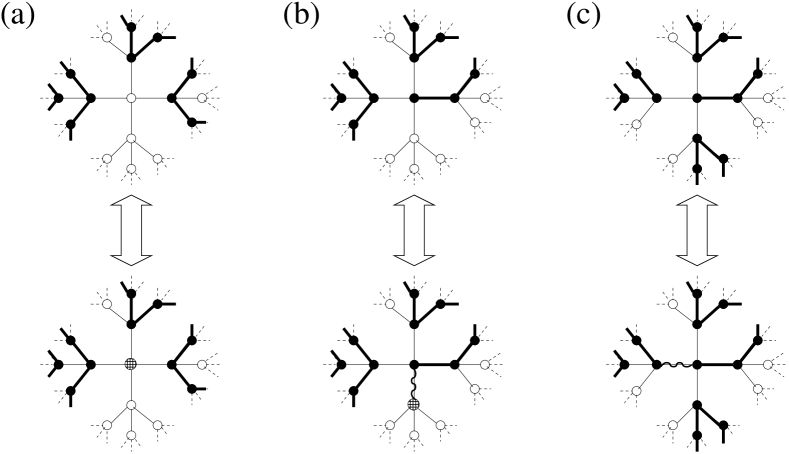
Figure 18: The three moves used in our Monte Carlo simulations on the Bethe lattice. The monomers (chain links) which change because of the move are represented with hatched circles (wiggly lines).

As already mentioned in Sec. V.4, numerical simulations of long fixed-length polymers are quite difficult on the Bethe lattice. We thus resort to simulating the variable-length ensemble corresponding to the free-energy (101). The algorithm includes three types of moves illustrated graphically in Fig. 18: (a) monomer insertion/deletion; (b) chain extension/reduction; (c) two chain junction/disjunction. It is straightforward to show that these three moves ensure ergodicity.

At each step of the algorithm the type of move and the location in the graph are chosen randomly. The move is then accepted according to the Metropolis rule in such a way as to satisfy detailed balance with respect to the variable length ensemble (101). Evidently the algorithm is more efficient for moderate lengths of the polymers, i.e., not too large values of $|\mu_{\rm end}|$. It can be therefore convenient, for producing equilibrated configurations, to gradually decrease $|\mu_{\rm end}|$ to the desired value.

Appendix G Numerical solution of the 1RSB cavity equations with population dynamics

The cavity recursion equation in the form (24) suggests a numerical solution by an iterative population dynamics cavityT : The distribution of local fields $\rho({\bf p})$ is represented by a (finite) population of fields. An iteration step in the dynamics consists in choosing at random $k$ “parent” members ${\bf p}^{(i)}$ of the population and calculating the corresponding cavity field ${\bf p}^{(0)}=I(\{{\bf p}^{(i)}\})$ from (4)-(7). This new field is then exchanged against an old field in the population with probability ${C[\{p^{(i)}\}]^{m}}/C_{\rm max}^{m}$, proportional to the reweighting $C[\{p^{(i)}\}]^{m}$ (normalized so as to make sure that the probability never exceeds 1). If the dynamics converges to a stationary distribution, its density satisfies the recursion equation (24).

In the soft glass phase, the iteration converges rapidly since the distribution of fields remains centered around the unstable liquid fixed point. However, the algorithm considerably slows down in the frozen phase where the fields have strong biases towards given conformations. Since the biases of the $k$ parent members are only rarely compatible with each other, the reweighting is usually very small. The population dynamics is then dominated by rare events with a low degree of frustration. Obviously, the probability of frustrated events rapidly increases with the number of different local conformations and thus with the length of the period $L$. For this reason we have limited our numerical simulations in the frozen glass phase to populations of 4000 fields for chains with $L=20$.

References

- [1] F. Aguilera-Granja and R. Kikuchi. Polymer statistics. I. Phase separation in polymer solutions : A new statistical treatment. Physica A, 176:514–533, 1991.
- [2] F. Aguilera-Granja and R. Kikuchi. Polymer statistics. II. New simulation of polymers in solution. Physica A, 182:331–345, 1992.
- [3] F. Aguilera-Granja and R. Kikuchi. Polymer statistics. III. Polymer adsorption on a solid surface. Physica A, 189:81–107, 1992.
- [4] F. Aguilera-Granja and R. Kikuchi. Polymer statistics. IV. Simulation of adsorption of polymers and polyelectrolytes on surfaces. Physica A, 189:108–126, 1992.
- [5] F. Aguilera-Granja and R. Kikuchi. Polymer statistics V. Simulation of polyelectrolytes adsorbed on negative surface. Physica A, 195:53, 1993.
- [6] U. Bastolla and P. Grassberger. Exactness of the annealed and the replica symmetric approximations for random heteropolymers. Phys. Rev. E, 63:031901, 2001.
- [7] R. N. Bhatt and A. P. Young. Numerical studies of Ising spin glasses in two, three, and four dimensions. Phys. Rev. B, 37:5606–5614, 1988.
- [8] J.-P. Bouchaud, L. Cugliandolo, J. Kurchan, and M Mézard. Out of equilibrium dynamics in spin glasses and other glassy systems. In A. P. Young, editor, Spin Glasses and Random Fields. World Scientific, Singapore, 1998.
- [9] J. Bryngelson, J. Onuchic, N. Socci, and P. Wolynes. Funnels, pathways, and the energy landscape of protein folding: A synthesis. Proteins: Struct. Funct. Genet., 21:167–195, 1995.
- [10] J. D. Bryngelson and P. G. Wolynes. Spin glasses and the statistical mechanics of protein folding. Proc. Nat. Acad. Sci, USA, 84:7524–7528, 1987.
- [11] H. S. Chan and K. A. Dill. Intrachain loops in polymers: effects of excluded volume. J. Chem. Phys., 90:493–509, 1989.
- [12] P. G. de Gennes. Collapse of a polymer chain in poor solvents. J. Phys. Lett. (Paris), 36:L55–L57, 1975.
- [13] P.G. de Gennes. Theory of long-range correlations in polymer melts. Faraday Discuss. Chem. Soc., 68:96, 1979.
- [14] B. Derrida. Random-energy model: An exactly solvable model of disordered systems. Phys. Rev. B, 24:2613–2626, 1981.
- [15] K. A. Dill. Theory for the folding and stability of globular proteins. Biochemistry, 24:1501, 1985.
- [16] A. V. Dobrynin and I. Ya. Erukhimovich. Fluctuation theory of random copolymers. J. Phys. France, 5:365–377, 1995.
- [17] R. Elber, editor. Recent Developments in Theoretical Studies of Proteins. World Scientific, Singapore, 1996.
- [18] G. H. Fredrickson, S. T. Milner, and L. Leibler. Multicritical phenomena and microphase ordering in random block copolymer melts. Macromolecules, 25:6341–6354, 1992.
- [19] T. Garel, L. Leibler, and H. Orland. Random hydrophilic hydrophobic copolymers. J. Phys. II (France), 4:2139–48, 1994.
- [20] T. Garel and H. Orland. Mean field model for protein folding. Europhys. Lett., 6:307–10, 1988.
- [21] T. Garel, H. Orland, and E. Pitard. Protein folding and heteropolymers. In A.P. Young, editor, Spin Glasses and Random Field, pages 387–443. World Scientific, Singapore, 1997.
- [22] E. N. Govorun, V. A. Ivanov, A. R. Khokhlov, P. G. Khalatur, A. L. Borovinsky, and A. Yu. Grosberg. Primary sequences of proteinlike copolymers: Levy-flight-type long-range correlations. Phys. Rev. E, 64:040903, 2001.
- [23] P. Grassberger and R. Hegger. On the collapse of random copolymers. Europhys. Lett., 31:351–356, 1995.
- [24] P. Grassberger and R. Hegger. Simulations of -polymers in 2 dimensions. J. Phys. I, 5:597, 1995.
- [25] A. M. Gutin, C. D. Sfatos, and E. I. Shakhnovich. Fluctuation effects on microphase separation in random copolymers. J. Phys. A, 27:7957–7968, 1994.
- [26] A. M. Gutin and E. I. Shakhnovich. Ground-state of random copolymers and the discrete random energy-model. J. Chem. Phys., 98:8174–8177, 1993.
- [27] K. Hukushima and K. Nemoto. Exchange Monte Carlo method and application to spin glass simulations. J. Phys. Soc. Jpn., 65:1604, 1996.
- [28] A. Irbäck, C. Peterson, and F. Potthast. Evidence for nonrandom hydrophobicity structures in protein chains. Proc. Natl. Acad. Sci. USA, 93:9533–9538, 1996.
- [29] A. Irbäck, C. Peterson, and F. Potthast. Identification of amino acid sequences with good folding properties in an off-lattice model. Phys. Rev. E, 55:860–867, 1997.
- [30] A. Irbäck, C. Peterson, F. Potthast, and O. Sommelius. Local interactions and protein folding: A three-dimensional off-lattice approach. J. Chem. Phys., 107:273–281, 1997.
- [31] Y. Kantor and M. Kardar. Collapse of randomly self-interacting polymers. Europhys. Lett., 28:169–174, 1994.
- [32] Alexei R. Khokhlov and Pavel G. Khalatur. Conformation-dependent sequence design (engineering) of AB copolymers. Phys. Rev. Lett., 82:3456–3459, 1999.
- [33] R. Kikuchi. A theory of cooperative phenomena. Phys. Rev., 81:988–1003, 1951.
- [34] T. R. Kirkpatrick and P. Wolynes. On the connection between some kinetic and equilibrium theories of glasses. Phys. Rev. A, 35:3072–3079, 1987.
- [35] K. Kremer, A. Baumgartner, and K. Binder. Collapse transition and crossover scaling for self-avoiding walks on the diamond lattice. J. Phys. A, 15:2879–2897, 1982.
- [36] S. Lise, A. Maritan, and A. Pelizzola. Bethe approximation for a semiflexible polymer chain. Phys. Rev. E, 58:R5241, 1998.
- [37] A. V. Lopatin and L. B. Ioffe. Structural glass on a lattice in the limit of infinite dimensions. Phys. Rev. B, 66:174202, 2002.
- [38] E. Marinari. Optimized Monte Carlo methods. In J. Kertész and I. Kondor, editors, Advances in computer simulations, page 50, Berlin, 1998. Springer.
- [39] M. Mézard and G. Parisi. The Bethe lattice spin glass revisited. Eur. Phys. J. B, 20:217, 2001.
- [40] M. Mézard and G. Parisi. The cavity method at zero temperature. J. Stat. Phys, 111:1, 2003.
- [41] P. Monari and A. L. Stella. -point universality of random polyampholytes with screened interactions. Phys. Rev. E, 59:1887–1892, 1999.
- [42] R. Monasson. Structural glass transition and the entropy of the metastable states. Phys. Rev. Lett., 75:2847–2850, 1995.
- [43] A. Montanari, M. Müller, and Mézard. The phase diagram of random heteropolymers. 2003. cond-mat/0307040.
- [44] A. Montanari, G. Parisi, and F. Ricci-Tersenghi. Instability of one-step replica-symmetry-broken phase in satisfiability problems. cond-mat/0308147.
- [45] A. Montanari and F. Ricci-Tersenghi. On the nature of the low-temperature phase in discontinuous mean-field spin glasses. Eur. Phys. J. B, 33:339, 2003.
- [46] A. Moskalenko, Yu. A. Kuznetsov, and K. A. Dawson. Glass transition of an amphiphilic random copolymer and relation to the Ising model of spin-glass. Europhys. Lett., 40:135–140, 1997.
- [47] J.F. Nagle. Statistical mechanics of the melting transition in lattice models of polymers. Proc. Roy. Soc. Lond. A, 337:569, 1974.
- [48] J. N. Onuchic, Z. A. Luthey-Schulten, and P. G. Wolynes. Theory of protein folding: An energy landscape perspective. Ann. Rev. Phys. Chem., 48:545–600, 1997.
- [49] V. S. Pande, A. Y. Grosberg, and T. Tanaka. Thermodynamic procedure to synthesize heteropolymers that can renature to recognize a given target molecule. Proc. Nat. Acad. Sci, USA, 91:12976–12979, 1994.
- [50] V. S. Pande, A. Y. Grosberg, and T. Tanaka. Heteropolymer freezing and design. Rev. Mod. Phys., 72:259–314, 2000.
- [51] V. S. Pande, A. Yu. Grosberg, and T. Tanaka. Nonrandomness in protein sequences: Evidence for a physically driven stage of evolution? Proc. Natl. Acad. Sci. USA, 91:12972–12975, 194.
- [52] Steven S. Plotkin, Jin Wang, and Peter G. Wolynes. Correlated energy landscape model for finite, random heteropolymers. Phys. Rev. E, 53:6271–6296, 1996.
- [53] T. Prellberg and A. L. Owczarek. Four-dimensional polymer collapse: Pseudo-first-order transition in interacting self-avoiding walks. Phys. Rev. E, 62:3780–3789, 2000.
- [54] M. Pretti. Bethe approximation for a hydrophobic-polar random copolymer. Phys. Rev. E, 66:031803, 2002.
- [55] M. Pretti. Semiflexible polymer in the cactus approximation. Phys. Rev. E, 66:061802, 2002.
- [56] D. Rose, A. Yu. Grosberg, T. Tanaka, and M. Rubinstein. Unexpected scenario of glass transition in polymer globules: an exactly enumerable model. Phys. Rev. Lett., 84:2417–2420, 2000.
- [57] C. D. Sfatos, A. M. Gutin, and E. I. Shakhnovich. Phase diagram of random copolymers. Phys. Rev. E, 48:465–475, 1993.
- [58] C. D. Sfatos and E. I. Shakhnovich. Statistical mechanics of random heteropolymers. Phys. Rep., 288:77–108, 1997.
- [59] E. I. Shakhnovich and A. M. Gutin. Formation of unique structure in polypeptide chains. Theoretical investigation with the aid of replica approach. Biophys. Chem., 34:187–199, 1989.
- [60] E. I. Shakhnovich and A. M. Gutin. The nonergodic (“spin-glass-like”) phase of heteropolymer with quenched disordered sequence of links. Europhys. Lett., 8:327–332, 1989.
- [61] E. I. Shakhnovich and A. M. Gutin. Enumeration of all compact conformations of copolymers with random sequence of links. J. Chem. Phys., 93:5967–5971, 1990.
- [62] E. I. Shakhnovich and A. M. Gutin. Engineering of stable and fast-folding sequences of model proteins. Proc. Nat. Acad. Sci, USA, 90:7195–7199, 1993.
- [63] H. Taketomi, Y. Ueda, and N. Go. Studies on protein folding, unfolding, and fluctuations by computer simulations. Int. J. Pept. Protein Res., 7:445–459, 1975.
- [64] M.C. Tesi, E.J. Janse van Rensburg, E. Orlandini, and S.G. Whittington. Interacting self-avoiding walks and polygons in three dimensions. J. Physics A, 29:2451, 1996.
- [65] D. Thirumalai, V. Ashwin, and J. K. Bhattacharjee. Dynamics of random hydrophobic-hydrophilic copolymers with implications for protein folding. Phys. Rev. Lett., 77:5385–5388, 1996.
- [66] E. G. Timoshenko, Yu. A. Kuznetsov, and K. A. Dawson. Kinetics of a Gaussian random copolymer as a prototype for protein folding. Phys. Rev. E, 54:4071–4086, 1996.
- [67] E. G. Timoshenko, Yu. A. Kuznetsov, and K. A. Dawson. Phase diagram of a Gaussian random copolymer. Phys. Rev. E, 55:5750–5758, 1997.
- [68] E. G. Timoshenko, Yu. A. Kuznetsov, and K. A. Dawson. Conformational transitions of heteropolymers in dilute solutions. Phys. Rev. E., 57:6801–6811, 1998.
- [69] P. G. Wolynes. Spin glass ideas and the protein folding problems. In D. Stein, editor, Spin Glass Ideas and Biology. World Scientific, Singapore, 1991.