Large stock price changes: volume or liquidity?

Abstract

We analyze large stock price changes of more than five standard deviations for i) TAQ data for the year 1997 and ii) order book data from the Island ECN for the year 2002. We argue that large price changes are not due to large trading volumes. Instead, we find that extreme price fluctuations are mainly caused by a low density of limit orders stored in the order book, i.e. a small liquidity.

The discovery of power law distributions for commodity Mandelbrot63 and stock price changes Lux96 ; Go+98 together with the relevance of this discovery for the practical problem of risk management has spurred a large amount of interest in the price process in financial markets. For physicists, the power law distribution of price changes is very appealing as the appearance of a power law is reminiscent of universality and critical phenomena, thus suggesting that there might be a basic and universal mechanism behind the distribution of price changes. Many phenomenological as well as microscopic models have been developed, which are able to explain the main stylized facts about financial time series Takayasu02 .

In order to understand the mechanism underlying the empirically observed return distribution in detail, one needs to study the price impact of trades. Besides the influence of news breaking, stock prices change if there is an imbalance between supply and demand. If more people want to buy than to sell, stock prices will move up, if more people want to sell than to buy, they will move down. This relation is quantified by the price impact function Hasbrouck91 ; HaLoMc92 ; kempf99 ; pler2002 ; Rosenow02 ; EvLy02 ; LiFaMa03 ; Ga+03 ; potbou2002 ; Hop02 ; Bou+03 , which describes stock price changes as a conditional expectation value of the order imbalance. The order imbalance is measured as the difference between the number of shares bought and the number of shares sold in a given time interval.

Gabaix et al. Ga+03 have suggested that large price changes are due to large order imbalances. Starting from the distribution of trading volumes and a fit to the average price impact function, they suggest an explanation for the empirical power law distribution of stock price changes. This approach was criticized in FaLi03 , because the test presented in Ga+03 lacks power in the presence of correlations in the order flow and because the functional form used to describe the price impact of large orders seems to vary for different stock markets. Instead, the authors of Fa+03 conclude from an event based analysis that large price changes are due to the granularity of the order book, which gives rise to a time varying liquidity.

Here, we present an empirical study of extreme stock price changes within time intervals of a length $\Delta t=5{\rm min}$. We analyze one year of data for the 44 most frequently traded NASDAQ stocks. These data are contained in the Trades and Quotes (TAQ) data base published by the New York Stock Exchange. In addition, we analyze one year of order book data from the Island ECN for the ten most frequently traded companies ticker . For both data bases, we find little evidence that price changes larger than five standard deviations are explained by the order imbalance. For the order book data, we are able to reconstruct the price impact function for time intervals with large price changes and find that price changes are quantitatively explained by unusually large slopes of the price impact function.

The TAQ data base contains information about transaction data like the number of shares and transaction price as well as information about quotes, i.e. the lowest sell offer (ask price $S_{\rm ask}(t)$) and the highest buy offer (bid price $S_{\rm bid}(t)$). The stock price change or return in a time interval $\Delta t$ is defined as

$$G(t)=\ln S_{\rm M}(t+\Delta t)-\ln S_{\rm M}(t),$$ (1)

where the midquote price $S_{\rm M}(t)={1\over 2}(S_{\rm bid}(t)+S_{\rm ask}(t))$ is the arithmetic mean of bid and ask price. The order imbalance $Q$ in a time interval is the sum of all signed market orders executed between $t$ and $t+\Delta t$. For the TAQ data, the sign of a transaction is determined by the Lee and Ready algorithm, which compares the transaction price to the midquote price. The sign is positive for buy orders (transaction price larger than midquote price) and negative for sell orders (transaction price smaller than midquote price). For the order book data, the data base contains information about the direction of a trade. We choose $\Delta t=5{\rm min}$. Returns $G$ are normalized by their standard deviation $\sigma_{G}$, volumes $Q$ by $\sigma_{Q}=\left\langle|Q-\langle Q\rangle|\right\rangle$ as their cumulative distribution function follows a power law with exponent close to two. The variance for data with such a distribution is not well defined.

Figure 1: (a) Average price impact function for the 44 most frequently traded NASDAQ stocks in the year 1997 with standard deviation of the mean. Price changes larger than five standard deviations cluster in the region of small volume imbalance, all of them are clearly outside the error bars. (b) Same as (a) but for 2002 data from the Island ECN order book for the ten most frequently traded stocks.

Average price impact and large events: The relation between price change and order imbalance is described by the price impact function

$$I_{\rm market}(Q)=\langle G_{\Delta t}(t)\rangle_{Q}\ \ .$$ (2)

It describes the average price change $G$ caused by an order imbalance $Q$ hidden in the same time interval.

We ask whether the average price impact function $I_{\rm market}(Q)$ is able to describe extremely strong price changes $G>5\;\sigma_{G}$. We determined all time intervals with price changes larger than five standard deviations and checked carefully that these large price changes are not due to errors in the data set but correspond to ”real” events. While the order book data seem to be free of errors, some errors are contained in the TAQ data. We have filtered the raw TAQ data against recording errors and apparent price changes due to the combination of data from different ECNs (electronic communications networks). We have used the algorithm of Chordia et al. chordia2001 , which discards all trades where the difference between trade price and midquote price is larger than 4 times the spread. The spread is defined as $S_{\rm ask}-S_{\rm bid}$. In addition, we have checked visually the return and trading volume time series surrounding the large price change on a tick by tick basis and have found no evidence for data errors after applying the filtering algorithm. The data filtering removes about one percent of all transactions and has a significant effect on the exponent of the cumulative distribution function $P(G>X)\sim x^{-\alpha}$. For the raw data without any filtering, we find $\alpha=2.1$, after applying the filter we find $\alpha=3.9$ by fitting a straight line in a double logarithmic diagram. We note that the filtering algorithm chordia2001 is very restrictive in the sense that it discards quite a few events where the TAQ data set reports erratic and strong oscillations (of several $\sigma_{G}$) of the price which are probably due to the combination of data from different ECNs. While the price has already reached its new ”true” value in the leading ECN, there may still be limit orders at the old price in some smaller ECNs which are exploited by arbitrage traders. While these oscillations are ”true” price changes in the sense that they are not due to recording errors, they are an artifact of the trading system and were not included in our analysis.

Figure 1 shows both the price impact function and those events with price changes larger than 5 standard deviations $\sigma_{G}$. We find 1198 such events for the TAQ data base and 210 for the Island ECN data. The large events cluster at quite small values of $Q$ where the price impact function is significantly below $G=5\sigma_{G}$. Surprisingly, for some of these events not even the sign of $Q$ and $G$ agree. We believe that this disagreement is mainly caused by the inaccuracy of the Lee and Ready algorithm, but the analysis of order book data reveals the existence of such situations as well. We note that even for large volume imbalances the average price impact function is several standard deviations (measured by the statistical error of the mean) below five $\sigma_{G}$ for the TAQ data.

Figure 2: Relation between the actual return $G$ and the predicted return $G_{\rm pred}$ as calculated from the average price impact function $I_{\rm market}(Q)$ and the actual order volume.

In Figure 2, the actual returns $G(t)$ are plotted against the predicted returns $G_{\rm pred}(t)=I_{\rm market}(Q(t))$ for the order book data. A linear fit to the data points has a slope of 2.58 indicating that the predicted returns are considerably smaller than the average one. The linear fit has an correlation coefficient $R^{2}=0.72$ and is not convincing visually. We conclude that the main cause for large returns is not a large imbalance between buy and sell orders but some other effect.

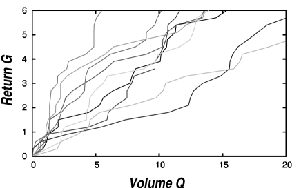
Figure 3: Price change as a function of buy or sell volume for ten of the largest price changes in the Island ECN data.

Time varying price impact: As the average price impact function does not provide for a satisfactory explanation of large returns, we study the time dependent price impact. In a modern electronic market place, market orders are matched with limit orders stored in the order book. A buy limit order indicates that a trader is willing to buy a specified number of shares at a given or lower price, while a sell limit order signals that a trader wants to buy a certain number of shares at a given or higher price. The buy limit order with the highest price determines the bid price, the sell limit order with the lowest price the ask price. The price change due to a given market order is determined by the limit orders stored in the order book. If a trader places a buy market order with volume $\Delta Q$, it executes as many limit orders as necessary to fill that volume. In this way, the order book determines the price change due to a single market order. We describe the order book by a density function $\rho_{\rm book}(\gamma,t)$, where the coordinate

$$\gamma=\left\{\begin{array}[]{ccc}(\ln(S_{\rm{limit}})-\ln(S_{\rm{bid}}))&\mbox{limit buy order}\\ (\ln(S_{\rm{limit}})-\ln(S_{\rm{ask}}))&\mbox{limit sell order}\end{array}\right.\ .$$ (3)

describes the position in the order book. In our analysis, the orderbook density is defined on a discrete grid with spacing $0.3\;\sigma_{G}$. A small market buy order with volume $\Delta Q$ causes a return $\Delta G$. For such an order, volume and return are related via $\Delta Q=\rho(0+,t)\Delta G$. For a larger order volume the relation is

$$Q=\int_{0}^{G}\rho(\gamma,t)\;d\gamma\ \ .$$ (4)

The return $G$ defined by Eq. 4 is denoted as the instantaneous or virtual price impact. From this relation one sees that the same order volume $Q$ can be related to quite different returns $G$ depending on the value of $\rho(\gamma,t)$. In the following, we will argue that it is this time dependence of the order book which is responsible for the occurrence of large price changes. We note that from the order book one obtains only information about the price change as a function of buy or sell volume. Order book information can be related to time aggregated signed order volumes only under the assumption i) that the order book is symmetric around the midquote price and that ii) nonlinearities can be neglected. Both assumptions are generally not satisfied. For this reason, we will consider either the buy or the sell volume in a given five minute interval, depending on the direction of the return in that interval.

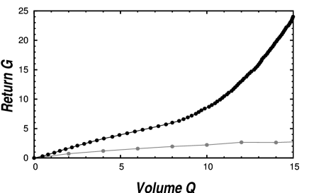
Figure 4: Average price change as a function of buy or sell volume for all price changes larger than $5\sigma_{G}$ in the Island ECN data. The average price change for all transactions is much smaller than that for the extreme events.

When studying the price impact of the order flow in a given time interval, it is not sufficient to invoke the order book density $\rho_{\rm book}(\gamma,t)$ at one instant of time. In addition, one has to consider changes in the order book which occur in this time interval. In WeRo03 it was shown that the virtual price impact of a given order volume is roughly four times stronger than the actual price impact. This difference is due to additional limit orders placed in reaction to a price change. From this example one sees that the inclusion of dynamical effects is crucial for calculating the correct price impact.

In order to calculate the density of additional limit orders arriving in a given time interval, we fix the reference frame by the midquote price in the beginning of the interval. The density of incoming limit orders is denoted by $\rho_{\rm flow}(\gamma,t)$, and the total order density is given by

$$\rho(\gamma,t)=\rho_{\rm book}(\gamma,t)+\rho_{\rm flow}(\gamma,t,\Delta t)\ \ .$$ (5)

From $\rho(\gamma,t)$ we calculate a price impact function $I_{\rm actual}(Q)$ by inverting the relation Eq. 4. The sell order side of this function for ten events with price changes larger than $5\sigma_{G}$ is shown in Figure 3. In Figure 4, the average over all such events is compared to the average price impact function $I_{\rm market}(Q)$. One sees that the slope of $I_{\rm actual}(Q)$ is much steeper than the slope of $I_{\rm market}(Q)$.

Figure 5: Ratio of actual price change to predicted price change plotted against the slope of the actual price impact function normalized by the slope of the average price impact function. The data points cluster in the vicinity of a linear fit.

The fact that the price impact function for large events has a steeper slope than the average price impact function implies that in time intervals with large price movements there are less limit orders available than on average. Hence, the slope of the actual price impact function provides a measurement of the market liquidity.

Some curves displayed in Figure 3 show marked nonlinearities. The exponents found from power law fits vary between 0.15 and 2.35 with a mean of 1.32 and a standard deviation of 0.41. However, the average of the $I_{\rm actual}$ for all large events (see Figure 4) is approximately linear, a power law fit yields an exponent of 1.03. As a measure for the strength of price impact, we define a susceptibility $\chi(t)$ for the actual price impact function for a given time interval by a linear fit up to a price change of $G=5\sigma_{G}$. Using this definition, we look for an explanation of extreme price changes. We compare the ratio of the actual price change $G(t)$ and the predicted price change

$$G_{\rm pred}(t)=I_{\rm market}(Q(t))\ \ .$$ (6)

to the ratio of actual slope $\chi(t)$ and slope $\chi_{\rm market}$ of the average price impact function $I_{\rm market}$. As explained above, a price impact calculated from the order book can only be defined for either buy or sell volume. For this reason, we have recalculated $I_{\rm market}$ by averaging with respect to either the sell or the buy volume, depending on the sign of the price change. This recalculated $I_{\rm market}$ is quite similar to the original one. To calculate $G_{\rm pred}(t)$, we use the buy volume for positive returns and the sell volume for negative ones.

In Figure 5 the ratio of $G_{\rm pred}$ and $G$ is plotted against the susceptibility $\chi/\chi_{\rm market}$ for all events with $|G|>5\sigma_{G}$. We see that the data points cluster in the vicinity of a straight line fit with an $R^{2}=0.74$. We conclude that the time dependent slope of the price impact function has a large explanatory power for the occurrence of extreme price changes.

In summary, we have studied two alternative approaches to explain large stock price changes: large fluctuations in trading volume and time changing liquidity for two different data sets. We find little evidence that extreme stock price changes are caused by large trading volume. For order book data, we are able to reconstruct the price impact for the time intervals with large returns. We find that the slope of this price impact strongly correlates with the ratio of observed return and the return predicted from the trading volume and the average price impact function.

References

- (1) B.B. Mandelbrot, J. Business 36, 394 (1963).
- (2) T. Lux, Appl. Financial Economics 6, 463 (1996); M. Loretan and P.C.B. Phillips, J. Empirical Finance 1, 211 (1994).
- (3) P. Gopikrishnan, M. Meyer, L.A.N. Amaral, and H.E. Stanley, Eur. Phys. J. B 3, 139 (1998).
- (4) H. Takayasu, ed., Empirical Analysis of Financial Fluctuations. Springer, Berlin, 2002.
- (5) J. Hasbrouck, J. Finance 46, 179-207 (1991).
- (6) J. Hausmann, A. Lo, and C. MacKinlay, J. Finan. Econ. 31, 319-379 (1992).
- (7) A. Kempf and O. Korn, J. Finan. Mark. 2, 29-48 (1999).
- (8) V. Plerou, P. Gopikrishnan, X. Gabaix, and H.E. Stanley, Physical Review E 66, 027104[1]-027104[4] (2002).
- (9) B. Rosenow, Int. J. Mod. Phys. C 13, 419-425 (2002).
- (10) M.D. Evans and R.K. Lyons, J. Political Economy 110, 170-180 (2002).
- (11) F. Lillo, J.D. Farmer, and R.N. Mantegna, Nature 421, 129 (2003).
- (12) X. Gabaix, P. Gopikrishnan, V. Plerou, and H.E. Stanley, Nature 423, 267-270 (2003).
- (13) M. Potters, J.-P. Bouchaud, Physica A 324, 133-140 (2003).
- (14) C. Hopman, Are supply and demand driving stock prices?, MIT working paper, Dec. 2002.
- (15) J.-P. Bouchaud, Y. Gefen, M. Potters, and M. Wyart, eprint cond-mat/0307332 (2003).
- (16) F. Lillo and J.D. Farmer, eprint cond-mat/0311053.
- (17) J.D. Farmer and F. Lillo, eprint cond-mat/0309416.
- (18) J.D. Farmer, L.Gillemot, F. Lillo, S. Mike, and A. Sen, eprint cond-mat/0312703 (2003).
- (19) C.M. Lee and M.J. Ready, J. Finance 46, 733-746 (1991).
- (20) We analyzed the following companies (ticker symbols): AMAT, BRCD, BRCM, CSCO, INTC, KLAC, MSFT, ORCL, QLGC, SEBL.
- (21) We do not include market orders executing ”hidden” limit orders in the definition of as we want to compare with the order book containing ”visible” orders only.
- (22) T. Chordia, R. Roll, and A. Subrahmanyam, J. Finance 56 (2), 501-530 (2001).
- (23) P. Weber and B. Rosenow, eprint cond-mat/0311457 (2003).