Phase Transition Strength through Densities
of General Distributions of Zeroes

Abstract

A recently developed technique for the determination of the density of partition function zeroes using data coming from finite-size systems is extended to deal with cases where the zeroes are not restricted to a curve in the complex plane and/or come in degenerate sets. The efficacy of the approach is demonstrated by application to a number of models for which these features are manifest and the zeroes are readily calculable.

1 Introduction

The study of phase transitions is central to statistical mechanics. Of primary interest is the determination of the location, the order and the strength of the transitions. While only systems of infinite extent display such phenomena, these are not directly accessible to the non-perturbative computational approach, which is restricted to a finite number of degrees of freedom. There are, however, well-established techniques for the extraction of information from numerical studies of finite systems, and prominent amongst them is finite-size scaling (FSS).

The FSS hypothesis is based on the premise that the only relevant scales are the correlation length of the infinite-size system and the linear extent of its finite-size counterpart [1]. A modification, in which the correlation length of the finite system replaces its actual size, extends the validity of the hypothesis to the upper critical dimension [2]. Traditional techniques to determine phase transition strength from finite-size data involve the application of FSS to thermodynamic quantities or to the lowest lying partition function zeroes [3].

However, a full understanding of the properties of the infinite-size system requires knowledge of the density of zeroes too. While it has long been expected that extraction of this quantity from finite-size systems would be a lucrative source of information, a technique to do so proved elusive [4]. The source of the difficulties is that it involves reconstruction of a continuous density function from a discrete data set, or sets, as the density of zeroes for a finite system is essentially a set of delta functions. Recent considerations have bypassed these difficulties [5, 6]. Rather than focusing on the density of zeroes itself, one determines the integrated density of zeroes. The robustness and efficiency of this approach was demonstrated in [5, 6] and the method favourably compared to other techniques in [7].

In these previous analyses, the distribution of zeroes had two special properties. These are (i) the zeroes dominating critical or pseudocritical behaviour lie on a curve called the singular line, which impacts onto the real axis at the transition point and (ii) these zeroes are simple zeroes (zeroes of order one). While these two properties are common to the bulk of models in statistical physics and in lattice field theory, they are by no means generic and the question of the generality of the technique presented in [5, 6] therefore arises.

The purpose of this paper is to extend the method presented in [5, 6] to deal with situations where the above two properties do not hold. Instead, the method developed here in Sec. 2 assumes the zeroes to be distributed across a two-dimensional region in the complex plane and/or to occur in degenerate sets. Such distributions of zeroes have been observed in various models of statistical physics and lattice field theory in two dimensions. The models we address in Sec. 3 are (a) the Ising model on a square lattice (using Brascamp-Kunz boundary conditions) with anisotropic couplings, (b) the Ising model on a bathroom-tile lattice, and (c) the case of free Wilson fermions in two dimensions. While all of these models are in the same two-dimensional Ising universality class, their detailed distributions of zeroes are quite different and provide a sufficiently wide sample to test the improved density-of-zeroes approach to the detection and characterization of phase transitions. Finally, Sec. 4 contains our conclusions.

2 Zeroes and their Densities

All of the information on a thermodynamical system in equilibrium is encoded in the zeroes of the appropriate partition function. Indeed, for a system of finite size, when the partition function, $Z_{L}$, can be written in as a polynomial in an appropriate function, $z$, of temperature, field or of a coupling parameter, we may write

$$Z_{L}(z)=A(z)\prod_{j}{\left(z-z_{j}(L)\right)}\quad,$$ (2.1)

where $L$ denotes the linear extent of the system, $j$ labels the zeroes, and $A(z)$ is a smooth non-vanishing function which plays no crucial role in the sequel and is henceforth discarded.

In numerical approaches to critical phenomena, FSS of the zeroes, $z_{j}(L)$ (with $j$ fixed – typically to $j=1$, which labels the zero nearest the transition point), is used to determine properties of phase transitions. A summary of the status of some of these calculations is given in [5]. On the other hand, attempts have also been made to gain a deeper understanding of some more tractable models analytically [8, 9]. Where these attempts have involved zeroes of the partition function, it is clear that much information is contained in their density. The technique developed in [5] is essentially a convergence of these two approaches, and we summarize it here for convenience.

2.1 Simple Zeroes on a Singular Line

The reduced free energy is obtained from (2.1) as

$$f_{L}(z)=\frac{1}{V}\ln{Z_{L}(z)}=\frac{1}{V}\sum_{j}{\ln{\left(z-z_{j}(L)\right)}}\quad,$$ (2.2)

having discarded the regular contribution coming from $A(z)$. Here $V$ represents the volume of the system. In independent series of publications, Abe [8] and Suzuki [9] assumed that the zeroes fall on a singular line in the complex plane, parameterized by $z=z_{c}+r\exp(i\phi)$, where $z_{c}$ is the transition point. In this case, a necessary and sufficient condition to achieve the correct scaling behaviour for the specific heat is that the density of zeroes along the singular line in the thermodynamic limit behave as $g_{\infty}{(r)}\propto r^{1-\alpha}$, where $\alpha$ is the usual critical exponent of the specific heat. Integrating, gives the cumulative density of zeroes in the infinite-volume limit,

$$G_{\infty}{(r)}\propto r^{2-\alpha}\quad.$$ (2.3)

In the finite-volume case, the density of zeroes is a string of delta functions, and,

$$g_{L}{(r)}=\frac{1}{V}\sum_{j}{\delta(r-r_{j}(L))}\quad,$$ (2.4)

where the $j^{\rm{th}}$ zero is given by $z_{j}(L)=z_{c}+r_{j}(L)\exp(i\phi)$. Integrating this along the singular line leads to the following expression for the cumulative density of zeroes [5, 6]:

$$G_{L}(r)=\left\{\begin{array}[]{cl}j/V&\mbox{if $r\in(r_{j},r_{j+1})$}\quad,\\ (2j-1)/2V&\mbox{if $r=r_{j}$}\quad.\end{array}\right.$$ (2.5)

The two central observations of [5, 6] were, firstly, that equating the infinite-volume density formula (2.3) to its finite-volume counterpart (2.5) is sufficient (with hyperscaling) to recover standard FSS expressions (indeed, FSS, traditionally the consequence of a hypothesis, emerges quite naturally from this approach), and, secondly, that (2.5) is a sensible definition of the cumulative density of zeroes in the finite case. With this definition, the strength of transitions may be directly measured by fitting to the ansatz

$$G(r)=a_{1}r^{a_{2}}+a_{3}\quad.$$ (2.6)

In particular, a non-zero value of $a_{3}$ indicates a definite phase. When $a_{3}$ vanishes, a transition of first order is indicated if $a_{2}\sim 1$, while a value of $a_{2}$ larger than $1$ indicates a second-order transition with strength

$$\alpha=2-a_{2}\quad.$$ (2.7)

In [5] and [6] this method was tested by application to a number of models in statistical physics and in lattice field theory. In all of these models, the locus of zeroes is one-dimensional, with a singular line impacting on the real axis at the transition point. Furthermore, all zeroes for finite lattices were simple zeroes (with no degeneracies). The question now arises as to how the technique translates to more general distributions of zeroes.

2.2 General Distribution of Zeroes

Departures from such smooth linear sets of zeroes were first observed for models on hierarchical and anisotropic two-dimensional lattices, for which there can exist a two-dimensional distribution (area) of zeroes [10, 11, 12]. Since then, a host of systems have been discovered with this feature [13, 14, 15, 16]. A common characteristic of all such two-dimensional distributions of zeroes is that the only physically relevant point at which they cross the real axis, in the thermodynamic limit, is that which corresponds to the phase transition. It is, however, possible that the zeroes cross the real or imaginary axis at unphysical points. These points may be associated with new universality classes.

Stephenson [17] has shown that the density of zeroes for such two-dimensional distributions in the infinite-volume limit is

$$g_{\infty}(x,y)=y^{1-\alpha-m}f\left(\frac{x}{y^{m}}\right)\quad,$$ (2.8)

where $(x,y)$ give the location of zeroes in the complex plane, with the critical point as the origin. Here $m$ is a new type of exponent which is related to the shape of the two-dimensional distribution [17].

Integrating out the $x$-dependence in (2.8) yields [17]

$$g_{\infty}(y)=\int_{x_{1}}^{x_{2}}{g_{\infty}(x,y)dx}\propto y^{1-\alpha}\quad,$$ (2.9)

where $x_{1}$ and $x_{2}$ mark the extremities of the distribution of zeroes at a distance $y$ from the $x$ axis in the complex plane. Integrating again, to determine the cumulative density of zeroes at the point $r$ in the $y$-direction, yields

$$G_{\infty}{(r)}\propto r^{2-\alpha}\quad,$$ (2.10)

an expression identical to (2.3). The strength of the transition, as measured by $\alpha$, can therefore be determined by similar methods to those previously used. However, rather than counting the zeroes along the singular line, one now counts them up to a line $y=r$ within the two-dimensional complex domain they inhabit.

The second new feature we wish to accommodate is the existence of degeneracies in the set of zeroes. If a number of zeroes coincide, $G_{L}$, as defined in (2.5), is multivalued and is no longer a proper function. A more appropriate density function is determined as follows. Suppose, in general, that $z_{j}=z_{j+1}=\dots=z_{j+n_{j}-1}$ are $n_{j}$-fold degenerate. By a glance at Fig. 1 it is easy to convince oneself that the densities to the left and right of an actual zero are given by

$$VG_{L}(r)=\left\{\begin{array}[]{ll}j+n_{j}-1&\mbox{for $r\in(r_{j+n_{j}-1},r_{j+n_{j}})$ \quad,}\\ j-1&\mbox{for $r\in(r_{j-1},r_{j})$ \quad.}\end{array}\right.$$ (2.11)

The density at the $n_{j}$-fold degenerate zero, $r_{j}$, is again sensibly defined as an average:

$$G_{L}(r_{j})=\frac{1}{V}\left(j+\frac{n_{j}}{2}-1\right)\quad.$$ (2.12)

This is the most general formula for extracting the density of any distribution of zeroes and deals with two-dimensional spreads and degeneracies. Fitting this quantity to the form (2.6) yields the strength of a second-order transition through (2.7). As in [5] and [6], the criteria for a good fit are good data collapse in $L$ (or $V$) and $j$ near the transition point and $a_{3}$ be compatible with zero.

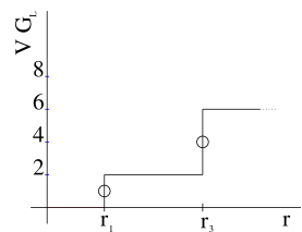
Figure 1: Schematic plot of cumulative density of zeroes as defined by (2.12). In this example, where the volume, $V$, is fixed, $r_{1}=r_{2}$ are $2$-fold degenerate, while $r_{3}=\dots=r_{6}$ are $4$-fold degenerate.

The error estimates appropriate to this modified density analysis may be determined from a procedure adapted from [5] and which we now elucidate. In the present case, where zeroes may be degenerate, the monotone nature of the cumulative density function means that the actual value of $G_{L}(r_{j}(L))$ cannot deviate from (2.12) by more than $\pm n_{j}/2V$ (see Fig. 1). The quantitative difference between this starting point and that in [5] is that this deviation is not constant in this case.

Let $G_{j}^{\rm{obs}}(L)$ represent the data point coming from the size-$L$ lattice and corresponding to the $j^{\rm{th}}$ zero, which is $n_{j}$-fold degenerate. Assign an initial error $\sigma_{j}(L)=\sigma_{\rm{arb}}n_{j}/V$ to this data point, where $\sigma_{\rm{arb}}$ is arbitrary. With these errors, the appropriate goodness-of-fit is given by

$$\chi_{1}^{2}=\sum_{L,j}{\frac{[G_{j}^{\rm{obs}}(L)-G_{j}^{\rm{exp}}(L)]^{2}}{\sigma_{j}(L)^{2}}}=\sum_{L,j}{\frac{V^{2}}{\sigma^{2}_{\rm{arb}}n_{j}^{2}}[G_{j}^{\rm{obs}}(L)-G_{j}^{\rm{exp}}(L)]^{2}}\quad,$$ (2.13)

where the expected density value, $G_{j}^{\rm{exp}}(L)$, comes from the model (2.6). Minimizing $\chi_{1}^{2}$ yields the parameters $a_{i}$ in (2.6) with associated errors denoted $da_{i}^{\rm{arb}}$.

Assume, now, the actual error associated with each data point is, in fact, $\sigma n_{j}/V$. The corresponding chi-squared may be written [5]

$$\chi_{2}^{2}=\frac{\sigma^{2}_{\rm{arb}}}{\sigma^{2}}\chi_{1}^{2}\quad.$$ (2.14)

If the model fits well, $\chi_{2}^{2}/N_{\rm{dof}}$ should be close to unity, where $N_{\rm{dof}}$ is the number of degrees of freedom. The error assigned to each point now becomes

$$\sigma^{2}=\sigma_{\rm{arb}}^{2}\chi_{1}^{2}/N_{\rm{dof}}=\chi_{1}^{2}/N_{\rm{dof}}\quad,$$ (2.15)

having chosen $\sigma_{\rm{arb}}$ to be unity. Moreover, the actual errors associated with the parameters $a_{i}$ are (with $\sigma_{\rm{arb}}=1$)

$$da_{i}=\frac{\sigma}{\sigma_{\rm{arb}}}da_{i}^{\rm{arb}}=\sigma da_{i}^{\rm{arb}}\quad.$$ (2.16)

Just as in [5], this approach prohibits an independent goodness-of-fit test.

In summary, the proceedure is to let $\sigma_{j}(L)=n_{j}/V$ and minimise $\chi_{1}^{2}$ in (2.13) to find $a_{i}$ and $da_{i}^{\rm{arb}}$. The best estimates for the errors are, then, $da_{i}=\sqrt{\chi_{1}^{2}/N_{\rm{dof}}}\,da_{i}^{\rm{arb}}$.

Note that standard FSS is for fixed-index zeroes and gives that the distance of a zero from the critical point is

$$r_{j}(L)\sim L^{-1/\nu}\quad.$$ (2.17)

Typically one uses the imaginary part of the zero, ${\rm{Im}}z_{j}$, for the distance $r_{j}$ in a traditional FSS analysis. The real part of the lowest zero may be considered as a pseudocritical point. Its scaling is characterised by the so-called shift exponent, $\lambda$, and

$${\rm{Re}}z_{1}(L)-z_{c}\sim L^{-\lambda}\quad,$$ (2.18)

where $z_{c}$ marks the critical point. Usually $\lambda$ coincides with $1/\nu$, but this is not always the case and the actual value of the shift exponent depends on the lattice topology. For a summary of some recent results concerning the finite-size shifting of the pseudocritical point in the Ising case in two dimensions, see [18].

3 Testing the Method on Various (Ising) Models

We take three two-dimensional models for which the zeroes are easily calculated. In each case the real, physical, critical point is in the Ising universality class, with strength of transition given by $\alpha=0$ (corresponding to a logarithmic divergence in the specific heat).

3.1 Square Lattice Ising Model with Anisotropic Couplings

The task of analytically solving the Ising model in two dimensions for finite-size systems is greatly ameliorated by the usage of Brascamp-Kunz boundary conditions [18, 19], where for an $M\times 2N$ lattice, the spins in the left boundary row at $x=0$ are fixed to $+$ and in the right boundary row at $x=M+1$ to the alternating sequence $+-+-\dots$, whereas in the $y$-direction periodic boundary conditions are assumed. In the general case of anisotropic couplings – $J_{1}$ along the $x$- and $J_{2}$ along the $y$-direction, with arbitrary ratio $R=J_{2}/J_{1}$ – the partition function takes the form [20]

$$Z_{M,2N}=2^{2NM}\prod_{i=1}^{M}\prod_{j=1}^{N}\left[\cosh(2\beta)\cosh(2R\beta)-\sinh(2\beta)\cos(\phi_{i})-\sinh(2R\beta)\cos(\theta_{j})\right]\quad,$$ (3.1)

where $\phi_{i}=i\pi/(M+1)$, $\theta_{j}=(2j-1)\pi/2N$, and $\beta=J_{1}/k_{B}T$. Recall that for fully periodic boundary conditions, the analogue of (3.1) consists of a sum of four product terms [21] which is much more cumbersome to analyze for the zeroes.

For isotropic couplings with $R=1$ the term in square brackets of (3.1) simplifies to $1-2\xi\sinh(2\beta)+\sinh^{2}(2\beta)$, with $-1\leq\xi=(\cos{\phi_{i}}+\cos{\theta_{j}})/2\leq 1$. It immediately follows that the complex zeroes can be parametrized exactly as $\sinh(2\beta)=\xi\pm i\sqrt{1-\xi^{2}}$, i.e., that they are distributed on the unit circle in the complex $\sinh(2\beta)$-plane.

For the anisotropic model with $R=3$, each factor in (3.1) can be rewritten as a fourth-order polynomial in $w=2\sinh(2\beta)$ to give

$$Z_{M,2N}=\prod_{i=1}^{M}\prod_{j=1}^{N}\left[w^{4}+5w^{2}+4-2w\cos(\phi_{i})-(6w+2w^{3})\cos(\theta_{j})\right]\quad.$$ (3.2)

The zeroes of (3.2) are also easily determined numerically, but it is not possible to parametrize them by a single variable, implying that they are distributed across a two-dimensional region rather than on a one-dimensional curve as in the isotropic case. In Fig. 2 this two-dimensional distribution of zeroes is shown for the case $R=3$

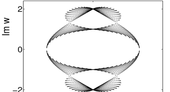
Figure 2: The partition function zeroes in the complex $w=2\sinh(2\beta)$ plane for the anisotropic ($J_{2}=3J_{1}$) $L=M=2N=40$ Ising model with Brascamp-Kunz boundary conditions.

and a square lattice of size $L=M=2N=40$.

The zeroes impact onto the real axis at the point $w=1$ and the critical behaviour is expected to be dominated by the zeroes close by. The zeroes in this case are all simple zeroes (no degeneracies), so it should be noted that this case is essentially a test of the applicability of the method to the situation of a two-dimensional distribution of zeroes in the complex plane rather than a test of how the method copes with varying degeneracies.

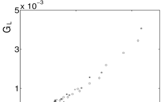
Figure 3: The distribution of zeroes near $w=1$ for the anisotropic Ising model with anisotropy ratio $R=3$ subject to Brascamp-Kunz boundary conditions for $L=40-140$ and $j=1$ ($\times$), $j=2$ ($+$), $j=3$ ($*$), $j=4$ ($\circ$), $j=5$ (  ), $j=6$ ($\diamond$), $j=7$ ($\bullet$), $j=8$ ($\star$).

The cumulative-density distribution for this set of zeroes is plotted in Fig. 3. A three-parameter fit to (2.6) for the first $8$ zeroes for lattices of size $L=40,60,80,100,120$, and $140$ gives $a_{3}=0.000002(15)$, indicating the presence of a transition. With $a_{3}$ set to zero, a two-parameter fit then yields $a_{2}=2.016(32)$, close to the expected value of $2$ (which corresponds to $\alpha=0$).

A closer inspection of Fig. 3 shows that the $j=1$ zeroes (denoted by the symbol $\times$) are slightly misaligned with respect to the higher-index zeroes. We have therefore repeated the fit restricted to $j=2-8$, which yields $G(r)=0.088(7)r^{2.008(33)}$, so that $\alpha=-0.008(33)$. This is nice confirmation that the technique works when the distribution of (non-degenerate) zeroes is two-dimensional.

Standard FSS applied to fixed-index zeroes using (2.17) yields the expected result, $\nu=1$ [18]. Similarly, the shift exponent in (2.18) is found to be $\lambda=2$. Thus $\lambda$ is not coincident with $1/\nu$. This contrasts with the case of the Ising model in two dimensions with toroidal boundary conditions [22] but matches results using topologies with a trivial fundamental homotopy group [23].

To understand these numerical results we return to the finite lattice expansion of (3.2) and look at the finite-size scaling of the lowest zero $w_{1}$, which is given by the roots of the factor in (3.2) with $i=j=1$ on an $M\times 2N$ lattice. For an infinite lattice the expression factorizes to give $(4+w^{2})(1-w)^{2}$ and we see the points where the distribution pinches down as the roots at $w=1$ (and at $w=\pm 2i$). For a finite square lattice ($L=M=2N$) we can expand around the root at $1$ in powers of ${1/L}$ to find

$$w=1+{\pi i\over L}-{\pi(2i+5\pi)\over 10L^{2}}+\cdots\quad.$$ (3.3)

Separating the real and imaginary parts yields ${\rm{Im}}w_{1}(L)\sim L^{-1}$ and ${\rm{Re}}w_{1}(L)-w_{c}\sim L^{-2}$.

For comparison, we present a similar analysis with anisotropy ratio $R=2$, for which the zeroes are plotted in Fig. 4. While the overall shape of the distribution is the same as in the $R=3$ case of Fig. 2, its detailed structure is different.

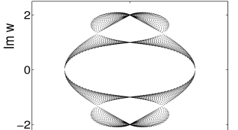
Figure 4: The partition function zeroes in the complex $w=2\sinh(2\beta)$ plane for the anisotropic ($J_{2}=2J_{1}$) $L=M=2N=40$ Ising model with Brascamp-Kunz boundary conditions.

In this case the density analysis reveals $a_{3}=-0.000\,01(2)$, and a subsequent two-parameter fit to the first $8$ zeroes for lattices of size $L=40$–$140$ yields $a_{2}=2.009(30)$, i.e. $\alpha=-0.009(30)$. The corresponding data is displayed in Fig. 5.

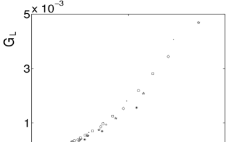
Figure 5: The distribution of zeroes near $w=1$ for the Ising model with anisotropy ratio $R=2$ subject to Brascamp-Kunz boundary conditions for $L=40-140$ and $j=1$ ($\times$), $j=2$ ($+$), $j=3$ ($*$), $j=4$ ($\circ$), $j=5$ (  ), $j=6$ ($\diamond$), $j=7$ ($\bullet$), $j=8$ ($\star$).

3.2 Bathroom-Tile Lattice

It is also possible to obtain two-dimensional distributions of zeroes for two-dimensional Ising models with isotropic couplings, one example being the Ising model on a bathroom-tile lattice [13]. This is the $(4\cdot 8^{2})$ lattice depicted in Fig. 6 and which is dual to the Union Jack lattice.

Figure 6: The bathroom tile lattice.

The continuum form of the (reduced) free energy on the bathroom-tile lattice is given by

$$f = \frac{3}{2}+\frac{1}{2}\ln(1+u)$$

$$+ \frac{1}{8}\int_{-\pi}^{\pi}\int_{-\pi}^{\pi}{{d\theta_{1}d\theta_{2}\over(2\pi)^{2}}\ln\left[A(u)+B(u)(\cos(\theta_{1})+\cos(\theta_{2}))+C(u)\cos(\theta_{1})\cos(\theta_{2})\right]}\quad,$$

where $u=\exp(-2\beta)$ and

$$A(u) = (1+u^{2})^{2}(1-4u+10u^{2}-4u^{3}+u^{4})\quad,$$

$$B(u) = 2u(1-u)^{3}(1+u)(1+u^{2})\quad,$$ (3.5)

$$C(u) = -4u^{2}(1-u)^{4}\quad.$$

This system is described in detail in [13]. The zeroes of the partition function were calculated from the finite lattice discretization of one of the terms in the partition function for periodic boundary conditions leading to (3.2), namely

$$Z = 2^{MN}\prod_{r=1}^{M}\prod_{s=1}^{N}\left\{A(u)+B(u)\left[\cos\left({2r-1\over M}\right)+\cos\left({2s-1\over N}\right)\right]\right.$$ (3.6)

$$+ \left.C(u)\cos\left({2r-1\over M}\right)\cos\left({2s-1\over N}\right)\right\}^{1/2}\quad.$$

In principle the full partition function is a sum of four such terms, differing in the arguments of the cosines which correspond to the four possible choices of (anti)periodic boundary conditions for the two species of fermions in the continuum limit of the model. In using (3.6), we are assuming that the scaling behaviour of one of these terms is generic. An alternative, which we do not pursue here as we are essentially interested in testing the scaling of the cumulative density of zeroes rather than formulating the finite lattice models themselves, would be to construct Brascamp-Kunz type boundary conditions for the bathroom tile lattice. This would also have the effect of projecting out a (different) single product term in the expression for $Z$.

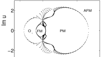
Figure 7: The partition function zeroes in the $u=\exp{(-2\beta)}$ plane for the bathroom-tile Ising model (3.6) with $L=M=N=40$. Here AFM, PM, FM and O₁ indicate the anti-ferromagnetic, paramagnetic, ferromagnetic and unphysical phases, respectively.

The phase diagram for such a system has paramagnetic [PM], ferromagnetic [FM] and anti-ferromagnetic [AFM] phases as well as an unphysical phase which we denote as O₁, to adhere to the same notation as [13]. The zeroes have varying degrees of degeneracy. Those for $L=M=N=40$ are depicted in Fig. 7 in the complex $u=\exp{(-2\beta)}$ plane and a blow-up of the region near the ferromagnetic critical point for $L=200$ is given in Fig. 8. Zeroes in the vicinity of the critical point taper off into a quasi-one-dimensional locus, so the bathroom-tile case is a test of the applicability of the method to zeroes of varying degeneracies, rather than to a true two-dimensional distribution.

The physical ferromagnetic critical point is given by $u=(1/2)\left(\sqrt{4\sqrt{2}-2}-\sqrt{2}\right)=0.249\,038\,4\dots$, corresponding to $\beta=0.695\,074\,1\dots$ [13]. In this region, the $j=1$ zeroes are four-fold degenerate, the $j=5$ are eight-fold degenerate, the $j=13$ zeroes are again four-fold, the $j=17$, $j=25$ and $j=33$ zeroes are each eight-fold degenerate, and the $j=41$ zeroes are four-fold degenerate.

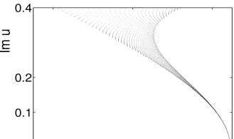
Figure 8: The bathroom-tile Ising zeroes near the ferromagnetic critical point $u=0.249\,038\,4\dots$ for $L=M=N=200$.

The cumulative density of zeroes near this ferromagnetic critical point is depicted in Fig. 9 for $L=40,70,100$, and $200$ with $j=1$–$44$ (seven data points for each $L$). A three-parameter fit to the form (2.6) clearly shows that the curve goes through the origin. Indeed, such a fit to the above data gives $a_{3}=0.000\,000\,7(830)$. Now, setting $a_{3}=0$, a two-parameter fit to the data yields $a_{2}=1.998(18)$, corresponding to $\alpha=0.002(18)$, fully consistent with zero, as expected.

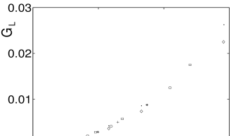
Figure 9: The distribution of zeroes for the bathroom-tile Ising model with $L=M=N=40-200$ and $j=1-4$ ($\times$), $j=5-12$ ($+$), $j=13-16$ ($*$), $j=17-24$ ($\circ$), $j=25-32$ (  ), $j=33-40$ ($\diamond$), $j=41-44$ ($\bullet$).

The physical antiferromagnetic critical point is given by $u=4.015\,445\,4\dots$, near which the zeroes again have a one-dimensional locus (as evident in Fig. 7). The degeneracy pattern for the first 44 zeroes is the same as in the above ferromagnetic critical case. A three-parameter fit yields $a_{3}=0.000\,01(3)$, and a two parameter fit to this data gives $a_{2}=2.03(2)$. Restricting the fit closer to the origin by using the $j=1-16$ (3 data points for each $L$) yields $a_{2}=1.9994(163)$, compatible with $\alpha=0$.

The accumulation point between the ferromagnetic and unphysical regions occurs at $u=-0.601\,231\,8\dots$ (for which there is no real $\beta$). Here the degeneracy pattern is different to those above, with the $j=1$ zeroes being four-fold degenerate, the $j=5$ zeroes eight-fold, the $j=13$ zeroes again four-fold, the $j=17$ and $j=25$ zeroes each eight-fold degenerate while the $j=33$ zeroes are four-fold and the $j=37$ zeroes are eight-fold degenerate. The density analysis again reveals a transition ($a_{3}=0$), with $a_{2}=2$ (e.g., the first 24 zeroes for $L=40-200$ give $a_{2}=1.993(12)$, corresponding to $\alpha=0.007(12)$).

A similar accumulation pattern occurs at the boundary between the antiferromagnetic and unphysical O₁ phases at $u=-1.663\,251\,9$, with the corresponding density analysis yielding $a_{2}=2.0095(123)$.

At each of the above four accumulation points, traditional FSS yields $\nu=1$ and $\lambda=2$.

3.3 Wilson Fermions

The partition function, $Z_{L}(\kappa)$ for a system of free Wilson fermions involves an integral over Grassmann variables, which, on completion, leads to the determinant of the Wilson matrix, $M^{\rm{(0)}}$. Here $\kappa=1/(2m_{0}+d)$ is the hopping parameter, $m_{0}$ is the dimensionless bare fermion mass and $d$ is the lattice dimensionality (which is $2$ in our case). It is well known that this system exhibits a phase transition at $1/2\kappa=d=2$, where massless fermions appear in the continuum limit [24]. This determinant may be expressed as a product of eigenvalues, and, for even lattice extent, $L$,

$$Z_{L}(\kappa)={\rm{det}}M^{(0)}=\prod_{\alpha=1}^{2}\prod_{p}\lambda_{\alpha}^{\rm{(0)}}(p)\quad,$$ (3.7)

where

$$\lambda_{\alpha}^{\rm{(0)}}(p)=\frac{1}{2\kappa}-\sum_{\mu=1}^{2}\cos{p_{\mu}}+i(-1)^{\alpha}\sqrt{\sum_{\mu=1}^{2}\sin^{2}{p_{\mu}}}\quad,$$ (3.8)

with $p_{\mu}=2\pi\hat{p}_{\mu}/L$ and where $\hat{p}_{1}=-(L-1)/2,-(L-3)/2,\dots,(L-1)/2$, while $\hat{p}_{2}=-L/2,-L/2+1,\dots,L/2$. These values comply with standard boundary requirements for Grassmann variables, namely that they are periodic in the spatial ($1$-) direction and antiperiodic in the temporal ($2$-) one [24].

The complex hopping-parameter zeroes are easily and exactly extracted from the multiplicative expression for the partition function (see [15]) and the zeroes for a system of size $L=50$ are depicted in Fig. 10 in the complex $1/2\kappa$ plane.

A special feature of Wilson fermions is the occurence of so-called doubler fermions. This means that apart from the physical critical point, which occurs where the zeroes accumulate at $1/2\kappa=2$ in the figure, there are lattice artefacts at $1/2\kappa=0$ and at $1/2\kappa=-2$ where further accumulations of zeroes, leading to critical behaviour, occur.

These Wilson-fermion zeroes clearly form a two-dimensional distribution. They also come in degenerate sets, with the first and seventh zeroes being 2-fold degenerate, while the third and nineth are 4-fold degenerate. So this system encapsulates both new features we seek to address.

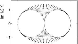
Figure 10: The partition function zeroes for the $L=50$ free Wilson fermions in the complex $1/2\kappa$ plane.

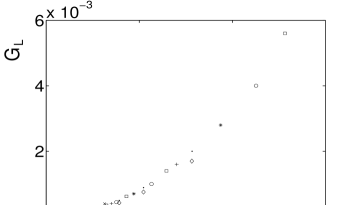
Figure 11: The distribution of zeroes near the physical critical point $1/2\kappa=2$ for free Wilson fermions with $L=50-250$ and $j=1-2$ ($\times$), $j=3-6$ ($+$), $j=7-8$ ($*$), $j=9-12$ ($\circ$), $j=13-16$ (  ), $j=17-18$ ($\diamond$), $j=19-23$ ($\bullet$).

The density plot for the zeroes near the physical transition is given in Fig. 11. Using the first twelve zeroes for lattices of size $L=50,100,150,200$, and $250$ (four data points for each lattice size), a three-parameter fit yields $a_{3}=0.000\,005(29)$, convincing evidence that the density plot indeed goes through the origin. The subsequent two-parameter fit yields $a_{2}={1.996(11)}$, giving $\alpha=0$, as expected.

It is worthwhile also applying the method to the artifactual doubler transition at $1/2\kappa=0$, where the two-dimensional nature of the distribution is more pronounced. There, the density data again fall on a universal curve (see Fig. 12) and $a_{3}$ is determined to be $0.000\,01(6)$. A two-parameter fit now yields $a_{2}={1.996(11)}$, again demonstrating that $\alpha$ is zero and the success of the method. Finally, as in the other systems studied here, traditional FSS yields $\nu=1$ and $\lambda=2$, so in each case the shift exponent does not match the inverse of the correlation-length exponent.

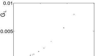
Figure 12: The distribution of zeroes near the artefactual critical point $1/2\kappa=0$ for free Wilson fermions with $L=50-250$ and $j=1-2$ ($\times$), $j=3-6$ ($+$), $j=7-8$ ($*$), $j=9-12$ ($\circ$).

4 Conclusions

A recently introduced technique to extract a continuous function, in the form of the density of partition function zeroes, from sets of discrete data has been extended to deal with the general case where (i) zeroes do not fall on a one-dimensional curve and/or where (ii) multiple zeroes may occur. The technique is tested in a variety of models which lie in the same universality class as the two-dimensional Ising model and which exhibit various combinations of these general features. It is seen to be capable of direct determination of the strength of the phase transition, as measured by the critical exponent $\alpha$. We have compared the results obtained from more standard finite-size scaling of the individual zeroes and also found good agreement.

It also perhaps worth highlighting that in this exercise we have found that formulating an Ising model with anisotropic couplings and Brascamp-Kunz boundary conditions is straightforward and still leads to a simple product form for the finite lattice partition function, a very useful property for investigating scaling. Though we have only touched on the topic briefly in this paper, the exotic critical points which appear at complex couplings in many models are also amenable to our analysis, and we discuss this elsewhere.

5 Acknowledgements

W.J. and D.J. were partially supported by EC IHP network “Discrete Random Geometries: From Solid State Physics to Quantum Gravity” HPRN-CT-1999-000161. RK would like to thank the Trinlat group at Trinity College Dublin for hospitality during an extended visit.

References

- [1] M.N. Barber, in: Phase Transitions and Critical Phenomena, Vol. 8, eds. C. Domb and J.L. Lebowitz (Academic Press, New York, 1971), p. 1; V. Privman, ed., A Collection of Reviews: Finite Size Scaling and Numerical Simulation of Statistical Systems (World Scientific, Singapore, 1990).
- [2] R. Kenna and C.B. Lang, Phys. Lett. B 264 (1991) 396; Nucl. Phys. B 393 (1993) 461; ibid. 411 (1994) 340 (Erratum); Phys. Rev. E 49 (1994) 5012.
- [3] C. Itzykson, R.B. Pearson, and J.B. Zuber, Nucl. Phys. B 220 (1983) 415.
- [4] P.P. Martin, Nucl. Phys. B 220 (1983) 366; ibid. 225 (1983) 497.
- [5] W. Janke and R. Kenna, J. Stat. Phys. 102 (2001) 1211; in: Computer Simulation Studies in Condensed-Matter Physics XIV, eds. D.P. Landau, S.P. Lewis, and H.-B. Schüttler (Springer, Berlin, 2002), p. 97.
- [6] W. Janke and R. Kenna, Nucl. Phys. B (Proc. Suppl.) 106-107 (2002) 905; Comp. Phys. Comm. 147 (2002) 443.
- [7] N.A. Alves, J.P.N. Ferrite, and U.H.E. Hansmann, Phys. Rev. E 65 (2002) 036110; N.A. Alves, U.H.E. Hansmann, and Y. Peng, Int. J. Mol. Sci. 3 (2002) 17.
- [8] R. Abe, Prog. Theor. Phys. 37 (1967) 1070; Prog. Theor. Phys. 38 (1967) 72; ibid. 322; ibid. 568.
- [9] M. Suzuki, Prog. Theor. Phys. 38 (1967) 289; ibid. 1225; ibid. 1243; Prog. Theor. Phys. 39 (1968) 349.
- [10] B. Derrida, Phys. Rev. B 24 (1981) 2613; B. Derrida, L. De Seze, and C. Itzykson, J. Stat. Phys. 33 (1983) 559.
- [11] W. van Saarlos and D. Kurtze, J. Phys. A 17 (1984) 1301.
- [12] J. Stephenson and R. Couzens, Physica 129A (1984) 201.
- [13] V. Matveev and R. Shrock, J. Phys. A 28 (1995) 5235.
- [14] W. Janke, D. Johnston, and R. Kenna, Nucl. Phys. B (Proc. Suppl.) 119 (2003) 882.
- [15] R. Kenna, C. Pinto, and J.C. Sexton, Nucl. Phys. B (Proc. Suppl.) 83 (2000) 667; Phys. Lett. B 505 (2001) 125; R. Kenna and J.C. Sexton, Phys. Rev. D 65 (2002) 014507.
- [16] Y.-L. Chou and M.C. Huang, Phys. Rev. E 67 (2003) 056109.
- [17] J. Stephenson, J. Phys. A 20 (1987) 4513.
- [18] W. Janke and R. Kenna, Phys. Rev. B 65 (2002) 064110; Nucl. Phys. B (Proc. Suppl.) 106-107 (2002) 929.
- [19] H.J. Brascamp and H. Kunz, J. Math. Phys. 15 (1974) 65.
- [20] B. Kastening, Phys. Rev. E 66 (2002) 057103.
- [21] B. Kaufman, Phys. Rev. 76 (1949) 1232.
- [22] A.E. Ferdinand and M.E. Fisher, Phys. Rev. 185 (1969) 832.
- [23] J. González and M.A. Martín Delgado, Preprint PUPT-1367 [hep-th/9301057]; Ch. Hoelbling and C.B. Lang, Phys. Rev. B 54 (1996) 3434.
- [24] I. Montvay and G. Münster, Quantum Field Theory on a Lattice (Cambridge University Press, Cambridge, 1994).