Information Geometry and Phase Transitions

Abstract

The introduction of a metric onto the space of parameters in models in Statistical Mechanics and beyond gives an alternative perspective on their phase structure. In such a geometrization, the scalar curvature, ${\mathcal{R}}$, plays a central role. A non-interacting model has a flat geometry (${\mathcal{R}}=0$), while ${\mathcal{R}}$ diverges at the critical point of an interacting one. Here, the information geometry is studied for a number of solvable statistical-mechanical models.

, and

1 Introduction

As the application of statistical-physics techniques becomes more widespread and acceptable outside the traditional physics community, it is clear that the phenomena of phase transitions have important roles to play there. Indeed, phase transitions are common to a very wide range of disciplines, from physics to biology, economics and even to sociology. As statistical physics finds pertinence in these areas, so too can the field draw on concepts outside the confines of pure physics.

In all of these disciplines, models are characterised by certain sets of parameters. The idea of endowing the space of such parameters with a metric and geometrical structure has been borrowed from parametric statistics [1]. Given a probability distribution $p(x|\theta)$, and a sample $x_{1},\dots,x_{n}$, the objective is to estimate the parameter $\theta$. This may be done by maximizing the so-called likelihood function, $L(\theta)=\prod_{i=1}^{n}{p(x_{i}|\theta)}$, or its logarithm (called the log-likelihood function),

$$\ln{L(\theta)}=\sum_{i=1}^{n}{\ln{p(x_{i}|\theta)}}\quad.$$ (1)

The gradient of this quantity is the score function:

$$U(\theta)=\frac{d\ln{L(\theta)}}{d\theta}\quad,$$ (2)

and the expectation of this random variable is zero (${\rm{E}}[U(\theta)]=0$). Its variance is

$${\rm{Var}}[U(\theta)]={\rm{E}}\left[\frac{-d^{2}\ln{L(\theta)}}{d\theta^{2}}\right]\quad.$$ (3)

This quantity is called the expected or Fisher information. Taylor expanding the log-likelihood function, one arrives at

$$\ln{L(\theta+\delta\theta)}-\ln{L(\theta)}=\delta\theta\left.\frac{d\ln{L(\theta)}}{d\theta}\right|_{\theta}+\frac{(\delta\theta)^{2}}{2}\left.\frac{d^{2}\ln{L(\theta)}}{d\theta^{2}}\right|_{\theta}+\dots\quad.$$ (4)

The first term on the right-hand side is zero at the true $\theta$-value. Therefore, the closeness of two probability distributions characterised by $\theta$ and $\theta+\delta\theta$, is given by the second term, or the Fisher information.

For higher-dimensional distributions (which may be continuous), where, instead of $\theta$, one has a set of parameters, $\theta_{1},\theta_{2},\dots$, the Fisher information is defined as

$$G_{ij}(\theta)=-E\left[\frac{\partial^{2}\ln{p(x|\theta)}}{\partial\theta_{i}\partial\theta_{j}}\right]=-\int{p(x|\theta)\frac{\partial^{2}\ln{p(x|\theta)}}{\partial\theta_{i}\partial\theta_{j}}dx}\quad.$$ (5)

C.R. Rao suggested this is a metric. It is, in fact, the only suitable metric in parametric statistics and is called the Fisher-Rao metric [1].

In generic statistical-physics models, we have two parameters, $\beta$, which we may think of as the inverse temperature, and $h$, the external field. In this case the Fisher-Rao metric is simply given by

$$G_{ij}=\partial_{i}\partial_{j}f\quad,$$ (6)

where $f$ is the reduced free energy per site and $\partial_{i}=(\partial/\partial\beta,\;\partial/\partial h)$.

For such a metric the scalar curvature may be calculated as

$${\mathcal{R}}\ =\ -\frac{1}{2G^{2}}\left|\begin{array}[]{ccc}\partial^{2}_{\beta}f&\partial_{\beta}\partial_{h}f&\partial_{h}^{2}f\\ \partial^{3}_{\beta}f&\partial_{\beta}^{2}\partial_{h}f&\partial_{\beta}\partial_{h}^{2}f\\ \partial^{2}_{\beta}\partial_{h}f&\partial_{\beta}\partial_{h}^{2}f&\partial_{h}^{3}f\end{array}\right|\quad,$$ (7)

where $G={\rm det}(G_{ij})$ is the determinant of the metric itself. The scalar curvature plays a central role in any attempt to look at phase transitions from a geometrical perspective. Indeed, ${\mathcal{R}}$ measures the complexity of the system. A flat metric implies that the system is not interacting. Conversely, and for all the models that have been considered so far, the curvature diverges at (and only at) a phase transition point for physical ranges of the parameter values.

Using standard scaling assumptions, we can anticipate the behaviour of ${\mathcal{R}}$ near a second-order critical point. With $t=1-\beta/\beta_{c}$,

$$f(\beta,h)=\lambda^{-1}f\left(t\lambda^{a_{t}},h\lambda^{a_{h}}\right)=t^{\frac{1}{a_{t}}}\psi\left(ht^{-\frac{a_{h}}{a_{t}}}\right)\quad,$$ (8)

where

$$a_{t}=\frac{1}{\nu d}\quad,\quad\quad\quad a_{h}=\frac{\beta\delta}{\nu d}\quad,$$ (9)

are the scaling dimensions for the energy and spin operators and $d$ is the spacial dimensionality. One finds for the scalar curvature,

$${\mathcal{R}}\ =\ -\frac{1}{2G^{2}}\left|\begin{array}[]{ccc}t^{\frac{1}{a_{t}}-2}&0&t^{\frac{1}{a_{t}}-2\frac{a_{h}}{a_{t}}}\\ t^{\frac{1}{a_{t}}-3}&0&t^{\frac{1}{a_{t}}-2\frac{a_{h}}{a_{t}}-1}\\ 0&t^{\frac{1}{a_{t}}-2\frac{a_{h}}{a_{t}}-1}&t^{\frac{1}{a_{t}}-3\frac{a_{h}}{a_{t}}}\end{array}\right|\quad,$$ (10)

and

$$G\sim t^{\frac{2}{a_{t}}+2\frac{a_{h}}{a_{t}}-2}\quad,$$ (11)

yielding

$${\mathcal{R}}\ \sim\xi^{d}\sim|\beta-\beta_{c}|^{\alpha-2}\quad,$$ (12)

where hyperscaling ($\nu d=2-\alpha$) is assumed and $\xi$ is the correlation length.

The systems hitherto analysed from the information-geometry perspective include the Ising model in one dimension [2], the Bethe lattice Ising and mean-field models [3]. The main results hitherto established are that ${\mathcal{R}}$ is positive definite and diverges (as $\xi^{d}$ ) only at the critical point.

In an effort to see how generic these features are, and to discover new ones, we analyse the Potts model in one dimension, the Ising model in two dimensions coupled to quantum gravity and the spherical model in three dimensions.

2 Information Geometry in Specific Models

The Potts Model in One Dimension: The one-dimensional $q$-state Potts model, like its Ising counterpart (which corresponds to $q=2$) is exactly solvable. Although it has no true phase transition, thermodynamic quantities diverge at zero temperature. In the Ising case, explicit calculations showed that

$${\mathcal{R}}_{\rm{Ising}}=1+\frac{\cosh{h}}{\sqrt{\sinh^{2}{h}+\exp{(-4\beta)}}}\quad.$$ (13)

The correlation length is known to behave as $\xi\sim-1/\ln{(\tanh{\beta})}$, and therefore ${\mathcal{R}}_{\rm{Ising}}\sim\xi$ as $\beta\rightarrow\infty$.

For plotting purposes, it is convenient to introduce

$$y=\exp{(\beta)}\quad\quad\quad{\rm{and}}\quad\quad\quad z=\exp{(h)}\quad.$$ (14)

The curvature is plotted in Fig. 1. It is clear that ${\mathcal{R}}_{\rm{Ising}}$ is positive definite and exhibits a $h\rightarrow-h$ (or $z\rightarrow 1/z$) symmetry. Furthermore, given a particular value for $y$, ${\mathcal{R}}_{\rm{Ising}}$ is maximum along the zero-field ridge $z=1$.

The one-dimensional $q$-state Potts model is also exactly solvable, so it is sensible to exploit it in an attempt to decide which of the previous features are generic. An explicit calculation [4] shows that

$${\mathcal{R}}_{\rm{Potts}}=A(q,y,z)+\frac{B(q,y,z)}{\sqrt{\eta(q,y,z)}}\sim y\sim\xi\quad,$$ (15)

for $h=0$ and $y\rightarrow\infty$. Here, $\eta(q,y,z)$ is the Potts analogue of the Ising term, $\sinh^{2}{h}+\exp{(-4\beta)}$, and $A$ and $B$ are smooth functions of $y$ and $z$. So the expected scaling (12) holds with $d=1$ or $\alpha=1$.

Figure 1 also shows that, in the Potts case, ${\mathcal{R}}_{\rm{Potts}}$ is no longer positive definite. Furthermore, the $z\rightarrow 1/z$ symmetry of the Ising model is no longer present. For a given $y$, ${\mathcal{R}}_{\rm{Potts}}$ no longer peaks along $z=1$. Finally, an analysis of the Lee-Yang (complex $h$) zeroes of the model reveals that the curvature also diverges as the locus of zeroes, $z_{0}(y)$, is approached. In fact,

$${\mathcal{R}}\sim\left(z-z_{0}(y)\right)^{-\frac{1}{2}}\quad,$$ (16)

so that this divergence is characterised by an edge exponent $\sigma=1/2$.

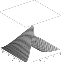
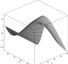
Figure 1: The scalar curvature for the Ising model (left) and the 10-state Potts model (right) in one dimension.

The Three-Dimensional Spherical Model (and the Ising Model on Planar Random Graphs): The spherical model is given by

$$Z_{\rm{spherical}}=\int{ds_{1}\dots ds_{L^{d}}\delta\left(\sum_{i}s_{i}^{2}-L^{d}\right)\exp{\left[\beta\sum_{\langle ij\rangle}{s_{i}s_{j}}+h\sum_{i}s_{i}\right]}}\quad,$$ (17)

and can be solved by exponentiating the constraint and using steepest descent. Allowing the lattice extent, $L$, to diverge reveals no transition for $d=1,2$. The transition for $d=3$ has $\alpha=-1$, $\beta=1/2$ and $\gamma=2$. This is the same set of critical exponents as for the Ising model on planar random graphs (matter coupled to 2D gravity). This is remarkable, because there are no obvious similarities between the two models.

Explicit calculations (in both models) give [5, 6]

$${\mathcal{R}}\sim|\beta-\beta_{c}|^{-2}\quad,$$ (18)

which does not accord with the prediction of (12). That prediction is ${\mathcal{R}}\sim|\beta-\beta_{c}|^{\alpha-2}$, with $\alpha=-1$. The source of the discrepancy can be traced back to the top left term in the determinant in (10), which is $t^{-\alpha}$. In both current models, $\alpha$ is, in fact, negative and this term vanishes as criticality is approached. It is replaced by a constant term coming from the regular part of the free energy. Both models then yield the same result (18).

3 Conclusions

In statistical physics, and in related fields – from the bio-sciences to economics – phase transitions play a central role. Thus new insights into the characterisation of critical phenomena are of paramount importance. Here, geometric ideas from the field of parametric statistics are “borrowed” and explored. It is found that the curvature associated with the Fisher-Rao metric is, indeed, a useful quantity in the characterisation of phase transitions. Some features found in the Ising model are found not to be generic. In particular, ${\mathcal{R}}$ can be negative and there is no symmetry nor ridge along $h=0$. More surprisingly, the naively expected scaling behaviour (12) fails in both the three-dimensional spherical model and in the Ising model on planar random graphs. Reasons for this are given. Once again, it is curious that all critical exponents for the latter two models coincide, although there is no obvious physical relation between them.

Acknowledgements: W.J. and D.J. were partially supported by EC IHP network “Discrete Random Geometries: From Solid State Physics to Quantum Gravity” HPRN-CT-1999-000161.

References

-
[1]
R.A. Fisher,
Phil. Trans. R. Soc. Lond. A 222 (1922) 309;
C.R. Rao, Bull. Calcutta Math. Soc. 37 (1945) 81. -
[2]
H. Janyszek, Rep. Math. Phys. 24 (1986) 1;
ibid. 11;
H. Janyszek and R. Mrugała, Phys. Rev. A 39 (1989) 6515. - [3] B.P. Dolan, Proc. Roy. Soc. London A 454 (1998) 2655.
- [4] B.P. Dolan, D.A. Johnston, and R. Kenna, J. Phys. A 35 (2002) 9025.
- [5] W. Janke, D.A. Johnston, and Ranasinghe P.K.C. Malmini, Phys. Rev. E 66 (2002) 056119.
- [6] W. Janke, D.A. Johnston, and R. Kenna, Phys. Rev. E 67 (2003) 046106.