Effects of two-site composite excitations in the Hubbard model

Abstract

The electronic states of the Hubbard model are investigated by use of the Composite Operator Method. In addition to the Hubbard operators, two other operators related with two-site composite excitations are included in the basis. Within the present formulation, higher-order composite excitations are reduced to the chosen operatorial basis by means of a procedure preserving the particle-hole symmetry. The positive comparison with numerical simulations for the double occupancy indicates that such approximation improves over the two-pole approximation.

url]http://www.scs.sa.infn.it

The analysis of highly correlated electron systems still reports many unsolved issues in spite of the large number of efforts which have been made for several decades. In general, difficulties come from the treatment of the collective excitations emerging in these systems, especially near the Mott-Hubbard transition. In this paper, we study the electronic states of the Hubbard model by use of the Composite Operator Method [1, 2, 3], which has shown to be capable to describe the physics of strongly correlated systems. Within projection techniques, going beyond the two-pole approximation, which implies the use of a local basis, is a very hard task. As first step along this direction, we here first used a four component operatorial basis with two non-local fields extending over two-sites.

The $d$-dimensional Hubbard Hamiltonian reads as follows,

$$H=\sum_{ij\sigma}(t_{ij}-\mu\delta_{ij})c^{\dagger}_{\sigma}(i)c_{\sigma}(j)+U\sum_{i}n_{\uparrow}(i)n_{\downarrow}(i),$$

where $c^{\dagger}_{\sigma}(i)$ and $c_{\sigma}(i)$ are creation and annihilation operators of electrons with spin $\sigma$ at the site $i$, respectively. $n_{\sigma}(i)=c^{\dagger}_{\sigma}(i)c_{\sigma}(i)$, $\mu$ is the chemical potential, $t_{ij}=-2dt\alpha_{ij}$, $\alpha[{\bf k}]=\mathcal{F}[\alpha_{ij}]=\frac{1}{d}\sum^{d}_{i=1}\cos(k_{i}a)$, $a$ is the lattice constant, $\mathcal{F}$ is the Fourier transform, $U$ is the on-site Coulomb repulsion. We define the following operatorial basis,

$$\psi_{\sigma}(i)=\left(\begin{array}[]{l}\xi_{\sigma}(i)\\ \eta_{\sigma}(i)\\ \xi_{s\sigma}(i)\\ \eta_{s\sigma}(i)\end{array}\right),$$ (1)

where $\xi_{\sigma}(i)=c_{\sigma}(i)\left(1-n_{-\sigma}(i)\right)$ and $\eta_{\sigma}(i)=c_{\sigma}(i)n_{-\sigma}(i)$ describe the transitions $n(i)=0$ $\leftrightarrow$ 1 and 1 $\leftrightarrow$ 2, respectively. $\xi_{s\sigma}(i)$ and $\eta_{s\sigma}(i)$ are

$$\begin{array}[]{l}\xi_{s\sigma}(i)=-n_{-\sigma}(i)\xi^{\alpha}_{\sigma}(i)+c^{\dagger}_{-\sigma}(i)c_{\sigma}(i)\xi^{\alpha}_{-\sigma}(i)\\ \hskip 39.83385pt+c_{\sigma}(i)\eta^{\alpha\dagger}_{-\sigma}(i)c_{-\sigma}(i)\vspace*{1mm}\\ \eta_{s\sigma}(i)=-n_{-\sigma}(i)\eta^{\alpha}_{\sigma}(i)+c^{\dagger}_{-\sigma}(i)c_{\sigma}(i)\eta^{\alpha}_{-\sigma}(i)\\ \hskip 39.83385pt+c_{\sigma}(i)\xi^{\alpha\dagger}_{-\sigma}(i)c_{-\sigma}(i)\end{array}$$ (2)

with $c^{\alpha}_{\sigma}(i)=\sum_{j}\alpha_{ij}c_{\sigma}(j)$. These operators describe two-site composite excitations which were not included in the previous work [2, 3], and are eigenoperators of the interaction term of the Hamiltonian, similarly to $\xi_{\sigma}(i)$ and $\eta_{\sigma}(i)$.

The equations of motion of the basis read as

$$\begin{array}[]{l}i\frac{\partial}{\partial t}\xi_{\sigma}(i)=-\mu\xi_{\sigma}(i)-zt\left[c^{\alpha}_{\sigma}(i)+\xi_{s\sigma}(i)+\eta_{s\sigma}(i)\right]\vspace*{1mm}\\ i\frac{\partial}{\partial t}\eta_{\sigma}(i)=(-\mu+U)\eta_{\sigma}(i)+zt\left[\xi_{s\sigma}(i)+\eta_{s\sigma}(i)\right]\vspace*{1mm}\\ i\frac{\partial}{\partial t}\xi_{s\sigma}(i)=-\mu\xi_{s\sigma}(i)\\ \hskip 19.91692pt-zt\left[-\frac{2}{z}\eta_{\sigma}(i)-\xi^{\alpha}_{s\sigma}(i)-2\eta^{\alpha}_{s\sigma}(i)+DJ_{\xi}(i)\right]\vspace*{1mm}\\ i\frac{\partial}{\partial t}\eta_{s\sigma}(i)=(-\mu+U)\eta_{s\sigma}(i)\\ \hskip 19.91692pt-zt\left[-\frac{1}{z}\eta_{\sigma}(i)-\xi^{\alpha}_{s\sigma}(i)+DJ_{\eta}(i)\right].\end{array}$$

where $z=2d$ is the coordination number. $DJ_{\xi}$ and $DJ_{\eta}$ are 3-site irreducible operators. By irreducible we mean that all local and two-site contributions have been subtracted. Hereafter, we will neglect $DJ_{\xi}$ and $DJ_{\eta}$. It is worth mentioning that the particle-hole symmetry of the model is preserved by this approximation. Then, the thermal retarded Green’s function $G({\bf k},\omega)=\mathcal{F}\langle\mathcal{R}[\psi(i)\ \psi^{\dagger}(j)]\rangle$ can be expressed as,

$$G({\bf k},\omega)=\sum_{n=1}^{4}\frac{\sigma_{n}({\bf k})}{\omega-E_{n}({\bf k})},$$ (3)

where

$$\begin{array}[]{l}E_{1}({\bf k})=-\mu-zt\alpha[{\bf k}]\\ E_{2}({\bf k})=-\mu-zt\alpha[{\bf k}]+U\\ E_{3}({\bf k})=-\mu+zt\alpha[{\bf k}]-zJ_{U}\\ E_{4}({\bf k})=-\mu+zt\alpha[{\bf k}]+U+zJ_{U},\end{array}$$ (4)

with $J_{U}=1/z(\sqrt{4zt^{2}+(U/2)^{2}}-U/2)$.

The spectral densities $\sigma_{n}({\bf k})$ contain two correlation functions: $\Delta=\langle\xi^{\alpha}_{\uparrow}(i)\xi^{\dagger}_{\uparrow}(i)\rangle-\langle\eta^{\alpha}_{\uparrow}(i)\eta^{\dagger}_{\uparrow}(i)\rangle$ and $p=\frac{1}{4}\langle n_{\nu}(i)n^{\alpha}_{\nu}(i)\rangle-\langle(c_{\uparrow}(i)c_{\downarrow}(i))^{\alpha}c^{\dagger}_{\downarrow}(i)c^{\dagger}_{\uparrow}(i)\rangle$. $\Delta$ can be directly computed in terms of the Green’s function. $p$ and $\mu$ are self-consistently evaluated through the constraint $\langle\xi(i)\eta^{\dagger}(i)\rangle=0$ and the equation defining the electron number density $\langle n\rangle$.

To test the reliability of the present approximation, we calculated the double occupancy $D=\langle n_{\uparrow}(i)n_{\downarrow}(i)\rangle$, and compared our results with the numerical data obtained by the Lanczos method for a 18-site system [4]. The agreement is considerably good over the whole $U/t$ range and the results show a clear improvement over the ones obtained by the two-pole approximation [3]. The details of the formulation and more extensive comparisons with numerical simulations will be presented elsewhere.

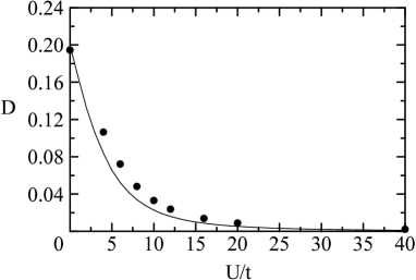
Figure 1: The double occupancy $D$ is reported as a function of $U/t$. $\langle n\rangle=8/9$ and the temperature $T=0$. Full circles represent the results of Ref. [4].

References

• [1] S. Ishihara, H. Matsumoto, S. Odashima, M. Tachiki, F. Mancini, Phys. Rev. B49 (1994) 1350.
• [2] F. Mancini, S. Marra, H. Matsumoto, Physica C244 (1995) 49; Physica C250 (1995) 184.
• [3] A. Avella, F. Mancini, Int. J. Mod. Phys. B17 (2003) 554.
• [4] F. Becca, A. Parola, S. Sorella, Phys. Rev. B61 (2000) 16287.