Infinite reflections of shock fronts in driven diffusive systems with two species

Abstract

Interaction of a domain wall with boundaries of a system is studied for a class of stochastic driven particle models. Reflection maps are introduced for the description of this process. We show that, generically, a domain wall reflects infinitely many times from the boundaries before a stationary state can be reached. This is in an evident contrast with one-species models where the stationary density is attained after just one reflection.

I Introduction

There are many intrinsically nonequilibrium phenomena which can be observed already in simplest systems of driven diffusing particles, a recent review of which can be found e.g. in Schu00 ; Liggett1999 ; Gunter_reviewJPA . Phase transitions induced by spatial boundaries of a system is one of those phenomena which was studied in detail for models with one-species of particles Krug91 ; Kolo98 ; Gunter_Slava_Europhys and for some multi-species models Mukamel95 ; Peschel . The ability of a nonequlibrium system to “feel” the boundaries constitutes a key feature of driven systems: in fact, the boundaries dominate the bulk giving rise to the phase transitions. It is a flux which brings information from the boundaries to the bulk: in absence of a flux, the boundary conditions play only a marginal role as one knows from equilibrium statistical mechanics.

A boundary problem in a one-dimensional driven diffusive system can be formulated as follows: the system is coupled at the ends to reservoirs of particles with fixed particle densities. A dynamics in the bulk and at the boundaries is defined via hopping rates, which are time-independent. In this case, after a certain transition period, the system will approach a stationary state, characteristics of which (the average flux, the density profile, the correlations) do not depend on time. It is of of interest how the system relax to the stationary state. Since a stationary state is independent on an initial state, one can choose an initial condition to be a domain wall interpolating between the boundaries. It has long been recognized that boundary-driven phase transitions are caused by the motion of a shock Kolo98 , so that the above initial choice is a very natural one. A key issue is to understand how the domain wall interacts with the boundaries. For the reference model in the field, an Asymmetric Simple Exclusion Process (ASEP) with open boundaries, a stationary density is reached after just one reflection, or interaction with a boundary.

We studied the reflection for the model with two conservation laws introduced in Peschel ; GunterJSP , and suprisingly observed infinitely many reflections occuring before a stationary state can be reached. More precisely, a domain wall after the first right reflection (i.e., the interaction with the right boundary) attains a different value of the density which is then changed after the first left reflection, etc.. This process continues iteratively. The bulk densities after multiple reflections asymptotically approach the stationary values.

Description of iterative reflection maps constitutes the main subject of the present paper.

Although the observed phenomenon of infinite reflections should be general, we use for the study a class of driven diffusive models having a simple stationary state on a ring for the sake of notational simplicity and to eliminate possible source of errors which may result from approximating a bulk flux, boundary conditions etc.. The findings are supported with Monte Carlo calculations and hydrodynamic limit analysis.

The paper is organized as follows: In section II we define the model and its symmetries and describe the stationary state on a ring. Hydrodynamic limit equations are given in section III. In section IV reflection maps are introduced and infinite iterative sequences are analyzed. Details concerning boundary rates can be found in the Appendix.

II The model

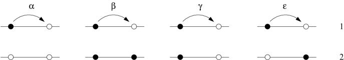
Figure 1: The four elementary hopping processes, shown here for one of the chains, and their rates. In the study, the rates are chosen to satisfy (1).

The model that we shall take as the example for our study is a particular case of a more general model introduced in Peschel ; GunterJSP , which can be viewed as a two-line generalization of ASEP. There are two parallel chains, chain $A$ and chain $B$ consisting of $N$ sites each. Any site can be empty or be occupied by a particle. The particle at a site $k$ can hop to its nearest right-hand site $k+1$ on the same chain provided it is vacant. The rate of hopping depends on the occupancy of the adjacent sites on the other chain, see Fig. 1. Hopping between the chains is forbidden. The hopping rates are fully symmetric with respect to an exchange between $A$ and $B$. Correspondingly, there are 4 different rates $\alpha,\beta,\gamma,\epsilon$ (see Fig. 1). However if one chooses them to satisfy $\alpha+\beta=2\gamma=2\epsilon$, then all particle configurations occur with the same probability in a stationary state (see GunterJSP ). In this case, the rate $\beta$ can be used to parametrize all the rates,

$$\alpha=1;\ \ \ \gamma=\epsilon=(1+\beta)/2.$$ (1)

Stationary fluxes on a ring with the densities $\rho^{A}$ and $\rho^{B}$ of the particles on the $A$ and $B$ -chain respectively are given in the thermodynamic limit (see GunterJSP ) by

$$\begin{array}[c]{cc}j^{A}(\rho^{A},\rho^{B})&=\rho^{A}(1-\rho^{A})(1+(\beta-1)\rho^{B})\\ j^{B}(\rho^{A},\rho^{B})&=\rho^{B}(1-\rho^{B})(1+(\beta-1)\rho^{A})\end{array}$$ (2)

For $\beta=1$ all the rates (1) become equal, which corresponds to an absence of an interaction between the chains, and the system splits into asymmetric exclusion processes ASEP ; ASEP1 ; Liggett1999 . Another choice of the rates $\alpha=\beta=\gamma\neq\epsilon$ was considered in Peschel .

The rates are by the definition nonnegative, so $\beta$ is in the range $0\leq\beta<\infty$. However it is sufficient to consider $0\leq\beta\leq 1$ because of a particle-hole symmetry. Indeed, an exchange of particles and holes plus the substitution $\beta\rightarrow 1/\beta$ leaves the model invariant.

In our context, we shall deal with a finite chains, where particles can be injected at the left end and be extracted at the right end of the system. We choose the boundary rates corresponding to effective stationary reservoirs of particles with fixed particle densities. Explicit expressions for the boundary rates are given, see the Appendix, in terms of the boundary densities. We denote the densities of $A(B)$-particles in the left boundary reservoir as $\rho_{L}^{A}(\rho_{L}^{B})$, and $\rho_{R}^{A}(\rho_{R}^{B})$ for the right boundary reservoir.

III Hydrodynamic limit

A naive continuum (Eulerian) limit of our stochastic dynamics on a lattice ${\hat{n}}_{k}(t)\rightarrow\rho^{\mathrm{A}}(x,t)$, ${\hat{m}}_{k}(t)\rightarrow\rho^{\mathrm{B}}(x,t)$ is a system of conservation laws

$${\frac{\partial\rho^{Z}(x,t)}{\partial t}}+{\frac{\partial j^{Z}(\rho^{\mathrm{A}},\rho^{\mathrm{B}})}{\partial x}}=\varepsilon{\frac{\partial^{2}\rho^{Z}}{\partial x^{2}}};\ \ \ Z=A,B,$$ (3)

$$\rho^{Z}(0,t)=\rho_{L}^{Z};\ \ \rho^{Z}(N,t)=\rho_{R}^{Z}$$

where on the right-hand side of (3) a phenomenological vanishing viscosity term has been added. This simplest regularization term leads to the correct answer for the Riemann problem, as compared to the stochastic model, see GunterJSP , but fails to describe a reflection from the boundaries (see Table 1). An adequate viscosity term is obtained by averaging of exact lattice continuity equations of the stochastic process

$${\frac{\partial}{\partial t}}\hat{n}_{k} =\hat{\jmath}_{k-1}^{\mathrm{A}}-\hat{\jmath}_{k}^{\mathrm{A}}$$ (4)

$${\frac{\partial}{\partial t}}\hat{m}_{k} =\hat{\jmath}_{k-1}^{\mathrm{B}}-\hat{\jmath}_{k}^{\mathrm{B}}$$ (5)

for occupation number operators $\hat{n}_{k},\hat{m}_{k}$, and taking the continuous limit $\langle\hat{n}_{k}\rangle\rightarrow\rho^{\mathrm{A}}(x,t)$, $\langle\hat{m}_{k+1}\rangle\rightarrow\rho^{\mathrm{B}}(x+a,t)$. For the case (1), the flux operator $\hat{\jmath}_{k}^{\mathrm{A}}$ reads (see GunterJSP )

$$\hat{\jmath}_{k}^{\mathrm{A}}=\hat{n}_{k}(1-\hat{n}_{k+1})\left(1+{\frac{\beta-1}{2}}\left(\hat{m}_{k}+\hat{m}_{k+1}\right)\right),$$ (6)

and $\hat{\jmath}_{k}^{\mathrm{B}}$ is obtained by an exchange $\hat{n}\leftrightarrow\hat{m}$ in the above. We substitute (6) into (4),(5), average, factorize and Taylor expand the latter with respect to a lattice spacing $a\ll 1$. In the first order of expansion, one obtains

$${\frac{\partial\rho^{\mathrm{A}}}{\partial t^{\prime}}}+{\frac{\partial j^{\mathrm{A}}(\rho^{\mathrm{A}},\rho^{\mathrm{B}})}{\partial x}} =\varepsilon{\frac{\partial}{\partial x}}\left(\left(1+(\beta-1)\rho^{\mathrm{B}}\right){\frac{\partial\rho^{\mathrm{A}}}{\partial x}}\right)$$ (7)

$${\frac{\partial\rho^{\mathrm{B}}}{\partial t^{\prime}}}+{\frac{\partial j^{\mathrm{B}}(\rho^{\mathrm{A}},\rho^{\mathrm{B}})}{\partial x}} =\varepsilon{\frac{\partial}{\partial x}}\left(\left(1+(\beta-1)\rho^{\mathrm{A}}\right){\frac{\partial\rho^{\mathrm{B}}}{\partial x}}\right)$$ (8)

$$\varepsilon={\frac{a}{2}}\rightarrow 0;\ \ {\frac{\partial}{\partial t}}=2\varepsilon{\frac{\partial}{\partial t^{\prime}}},$$ (9)

A numerical integration of (7),(8) shows that the dynamics of the stochastic process is described adequately. At the same time, predictions of (3) strongly disagree with the stochastic dynamics (see e.g. Table 1). Thus, in contradiction to the one-species case, where a choice of the vanishing viscosity is very robust, for a model with two and more species the specific choice of the viscosity becomes crucial: different choices give different answers.

IV Reflection maps

We explain our approach firstly for noninteracting chains $\beta=1$. In this case the dynamics of each chain reduces to the one of the ASEP with an injection rate $\rho_{L}$ and an extraction rate $(1-\rho_{R})$, see ASEP ; ASEP1 , corresponding to reservoirs of particles with densities $\rho_{L}$ and $\rho_{R}$ on the left and on the right boundary, see the Appendix. To study interaction with the right boundary, choose an initial state to be a homogeneous state $\langle\hat{n}_{k}\rangle=\rho_{bulk}=\rho_{L}$, for all $k$, matching perfectly the left boundary. Consequently the particle distribution at the left boundary will not change in time, while at the right boundary there is a mismatch if $\rho_{L}\neq\rho_{R}$, which has to be resolved. Monte-Carlo simulation shows that one of the following scenarios is realized, see Fig. 2: (a) a thin boundary layer develops interpolating between the bulk density $\rho_{\mathrm{bulk}}=\rho_{L}$ and $\rho_{R}$, and stays always attached to the right boundary, (b) a shock wave of the density $\rho_{R}$ develops and propagates to the left boundary, (c) a rarefaction wave with the density $\rho=max(\rho_{R},1/2)$ forms and spreads towards the left boundary.

Analogously, we study the left reflection, choosing an initial condition $\rho_{L}\neq\rho_{bulk}=\rho_{R}$. Then, the mismatch will be only at the left boundary. We can predict interaction results by exploiting a particle-hole symmetry of the model: an exchange of particles and holes and the left with the right boundary leaves the system invariant. Hence a dynamics of the model with $\rho_{L}=\rho_{bulk}\neq\rho_{R}$ is equivalent to a dynamics of the dual model

$$\rho_{L}^{\prime}\neq\rho_{bulk}^{\prime}=\rho_{R}^{\prime},\mathrm{where}\ \rho_{L}^{\prime}=1-\rho_{R},\ \rho_{R}^{\prime}=1-\rho_{L}:$$ (10)

The corresponding local densities of the dual model satisfy

$$\langle\hat{n}_{k}\rangle=\langle\hat{n^{\prime}}_{N-k+1}\rangle;\ \ k=1,2,\ldots N.$$ (11)

As an example, Fig. 2d shows the Monte Carlo evolution corresponding to shock propagation, dual to the one on Fig. 2b, through the transformations (10),(11). The other scenarios for the left reflection can be deduced from Fig. 2a,c, using (10),(11).

We shall classify an outcome of a reflection from a boundary by an average particle density $\rho_{refl}$ of the reflected wave measured at some point $k^{*}$ not too close to the boundary to avoid boundary effects. The density $\rho_{refl}$ is measured after the reflection wave has passed the point $k^{*}$ but before it has reached the other boundary, to avoid possible interference. For instance, reflected wave has the density $\rho_{refl}=\rho_{L}$ for the scenario (a), $\rho_{refl}=\rho_{R}$ for the scenario (b) and $\rho_{refl}=1/2$ for the scenario (c) on Fig. 2.

We can summarize the results of all possible reflections from the right boundary $\rho_{R}$ by plotting the density of the reflected wave versus the initial bulk density, see Fig. 3. We shall call this type of graph a reflection map. Reflection map for the left boundary is obtained using (10),(11). Comparing the reflection maps with the stationary phase diagram of ASEP ASEP ; ASEP1 , one can make an important observation. Namely, the stationary state density is achieved after one reflection from any of the boundaries. We have checked this statement to be true also for a two-parameter model with a next nearest neighbour interaction (KLS model), the stationary phase diagram of which is obtained in Gunter_Slava_Europhys .

In the following we show that for a two-component system it takes infinite number of reflections until the stationary density is reached.

IV.1 Two interacting chains

Consider the two-chain model (1) coupled to boundary reservoirs with the densities of $A$- and $B$- particles $\rho^{A}_{L},\rho^{B}_{L}$ and $\rho^{A}_{R},\rho^{B}_{R}$ at the left and at the right end respectively. Consider a reflection problem by choosing an initially homogeneous particle distribution with the densities

$$\rho^{A}_{\mathrm{bulk}}=\rho^{A}_{L};\ \ \rho^{B}_{\mathrm{bulk}}=\rho^{B}_{L}\ \ \mbox{ for the right reflection}$$ (12)

$$\rho^{A}_{\mathrm{bulk}}=\rho^{A}_{R};\ \ \rho^{B}_{\mathrm{bulk}}=\rho^{B}_{R}\ \ \mbox{ for the left reflection}$$ (13)

We shall classify results of a reflection as it was done above for ASEP. Denote the densities of the particles in the reflected wave in $A-$ and $B$-chain as $r^{A},r^{B}$. Suppose that after interaction with a boundary an interface appears between $\rho^{A}_{\mathrm{bulk}},\rho^{B}_{\mathrm{bulk}}$ and $r^{A},r^{B}$ moving towards the other boundary. Due to particle number conservation in the bulk, a $Z$-component of the interface moves with the velocity assume

$$V^{Z}={\frac{j^{Z}_{\mathrm{bulk}}-j^{Z}_{\mathrm{r}}}{\rho^{Z}_{\mathrm{bulk}}-r^{Z}}}\ ,$$ (14)

where we used the short notations $j^{Z}_{\mathrm{bulk}}=j^{Z}(\rho^{A}_{\mathrm{bulk}},\rho^{B}_{\mathrm{bulk}})$, $j^{Z}_{\mathrm{r}}=j^{Z}(r^{A},r^{B})$. Since there is an interaction between the chains, the velocities must coincide in both chains because a perturbation in one chain causes the response in the other and vice versa. This gives a restriction $V^{A}=V^{B}$, or

$${\frac{j^{A}_{\mathrm{bulk}}-j^{A}_{\mathrm{r}}}{\rho^{A}_{\mathrm{bulk}}-r^{A}}}={\frac{j^{B}_{\mathrm{bulk}}-j^{B}_{\mathrm{r}}}{\rho^{B}_{\mathrm{bulk}}-r^{B}}},$$ (15)

defining implicitly the allowed location of the points $r^{A},r^{B}$.

For demonstration purposes, we choose $\beta=0$ in (1) which corresponds to the maximal interchain interaction. This choice simplifies drastically analytic expressions and at the same time preserves qualitative features of the general case. For $\beta=0$, Eq.(15) has two families of solutions, given by

$$r^{A}/r^{B} =\rho_{\mathrm{bulk}}^{A}/\rho_{\mathrm{bulk}}^{B}$$ (16)

$$(1-r^{A})(1-r^{B}) =(1-\rho_{\mathrm{bulk}}^{A})(1-\rho_{\mathrm{bulk}}^{B})$$ (17)

It turns out that the densities of waves resulting from the interaction with the right boundary satisfy (16) while those resulting from the left reflection satisfy (17).

IV.1.1 Right reflection

Consider the right reflection (12) first. Monte Carlo simulations, independently confirmed by a continuous model integration, lead to the following conclusion:

the reflection densities $r^{A},r^{B}$ either coincide with the $\rho^{A}_{\mathrm{bulk}},\rho^{B}_{\mathrm{bulk}}$ (in this case boundary layers analogous to Fig. 2$a$ develop), or depend only on the ratio $\gamma=\frac{\rho^{A}_{\mathrm{bulk}}}{\rho^{B}_{\mathrm{bulk}}}$. In the latter case, $r^{B}(\gamma)/r^{A}(\gamma)=\gamma$, see (16). On Fig. 4, a typical dependence of $r^{A}$ on the initial bulk density along the line $\frac{\rho^{B}_{\mathrm{bulk}}}{\rho^{A}_{\mathrm{bulk}}}=\gamma$ is shown. Analogously to the left graph on Fig. 3, a discontinuos change of $r^{A}$ occurs, defining a point of a first order boundary driven phase transition other_case .

Collection of points $r^{A}(\gamma),r^{B}(\gamma)$ for all possible initial bulk densities $0\leq\gamma=\frac{\rho^{B}_{\mathrm{bulk}}}{\rho^{A}_{\mathrm{bulk}}}\leq\infty$, constitutes a continuous curve $\mathcal{R}$ shown on Fig. 5. The shape of $\mathcal{R}$ depends only on the right boundary densities $\rho^{A}_{R},\rho^{B}_{R}$. In the following we derive some analytical properties of $\mathcal{R}$, namely the coordinates of three points on $\mathcal{R}$ and the derivative in one of them.

Trivially $\mathcal{R}$ contains the point $\rho_{R}^{A},\rho_{R}^{B}$ corresponding to the perfect match with the right boundary. Then, the location of end points of $\mathcal{R}$ can also be derived. Indeed, consider the system with the empty $B$-chain: $\rho_{\mathrm{bulk}}^{B}=0$. Then, the model becomes effectively an ASEP, with the rate of extraction of the particles $t_{\mathrm{ext}}^{0}$ given by (A.9), which corresponds to the effective right boundary density in ASEP $\rho_{R}=1-t_{\mathrm{ext}}^{0}$. Consulting the reflection graph for ASEP Fig. 3, we find that corresponding reflected wave in the $A$-channel has the density $\max(1-t_{\mathrm{ext}}^{0},0.5)$. Thus, the curve $\mathcal{R}$ has a point with the coordinates $(\max(1-(1-\rho^{A}_{R})(1-\frac{1}{2}\rho_{R}^{B}),0.5),\ \ 0)$. Repeating the arguments for the empty $A$-chain $\rho^{A}_{bulk}=0$, we find the other end point on $\mathcal{R}$, $(0,\ \ \max(1-(1-\rho^{B}_{R})(1-\frac{1}{2}\rho_{R}^{A}),0.5))$.

Now, the exact derivative of $\mathcal{R}$ at the point $\rho_{R}^{A},\rho_{R}^{B}$ can also be derived. Indeed, it is shown in the section III that our system is described in the continuous limit by the system of equations (7,8). After the initial period of strong interaction with the right boundary, the distribution of particles near the boundary does not change anymore (see e.g. Fig.2 b), and can be described by a time-independent solution of (7,8). The current in the region will then be equal to that of the reflected wave. Integrating the time-independent part of Eq.(7) for $\beta=0$, one obtains:

$$j^{\mathrm{A}}(\rho^{\mathrm{A}}(x),\rho^{\mathrm{B}}(x))=j_{\mathrm{stat}}^{\mathrm{A}}(r^{\mathrm{A}},r^{\mathrm{B}})+\varepsilon{\frac{\partial\rho^{\mathrm{A}}}{\partial x}}\left(1-\rho^{\mathrm{B}}(x)\right)$$ (18)

where the current of the reflected wave $j_{\mathrm{stat}}^{\mathrm{A}}(r^{\mathrm{A}},r^{\mathrm{B}})$ is the constant of integration.

Suppose the result of the reflection $(r^{A},r^{B})$ differs only infinitesimally from the right boundary values, $r^{Z}\approx\rho_{R}^{Z}$, $\ Z=A,B$. The Taylor expansion of (18) around the $r^{A},r^{B}$ gives in the first order approximation

$${\left({\frac{\partial j^{\mathrm{A}}}{\partial\rho^{A}}}\right)}_{R}\delta\rho^{A}+{\left({\frac{\partial j^{\mathrm{A}}}{\partial\rho^{B}}}\right)}_{R}\delta\rho^{B}=\lambda\left(\delta\rho^{A}(1-\rho_{R}^{\mathrm{B}})\right)$$ (19)

where the subscript $R$ denotes evaluation at the point $\rho_{R}^{A},\rho_{R}^{B}$, and we suppose the profile $\rho^{Z}(x)$ to approach exponentially the values $r^{A},r^{B}$ from the right. An equation for the other flux component $j^{\mathrm{B}}$, obtained analogously, can be combined together with (19) into a modified eigen-value equation

$${\left(\mathcal{D}j\right)}_{R}{\binom{\delta\rho^{A}}{\delta\rho^{B}}}=\lambda\mathcal{B}{\binom{\delta\rho^{A}}{\delta\rho^{B}}};\ \ \ \mathcal{B}=\left(\begin{array}[c]{cc}1-\rho_{R}^{\mathrm{B}}&0\\ 0&1-\rho_{R}^{\mathrm{A}}\end{array}\right),$$ (20)

where $\mathcal{D}j$ is the Jacobian of the stationary flux (2) with the elements $\mathcal{D}_{UV}=\partial j^{U}/\partial\rho^{V}$. For any given value of the boundary densities, $\lambda$ is determined self-consistently, and the ratio $\delta\rho^{B}/\delta\rho^{A}$ is the derivative of the curve $\mathcal{R}$ at the point $\rho_{R}^{A},\rho_{R}^{B}$. The system (20) has two solutions, one is relevant for the right boundary reflection and one for the left reflection. The solution, relevant for the right reflection, reads for $\beta=0$:

$${\frac{\delta\rho^{B}}{\delta\rho^{A}}}={\frac{(1-\rho_{R}^{B})(\rho_{R}^{B}-\rho_{R}^{A}-\sqrt{(\rho_{R}^{A})^{2}+(\rho_{R}^{B})^{2}-\rho_{R}^{A}\rho_{R}^{B}})}{\rho_{R}^{A}(1-\rho_{R}^{A})}}.$$ (21)

We observe an excellent agreement between the theoretical and numerically evaluated values of ${\frac{\delta\rho^{B}}{\delta\rho^{A}}}$, see Table 1. The last column of the Table gives the value of ${\frac{\delta\rho^{B}}{\delta\rho^{A}}}$ which would follow from the “naive” viscosity term as written in (3), which leads correspondingly to $\mathcal{B}=I$ in (20), and to the expression $({\frac{\delta\rho^{B}}{\delta\rho^{A}})}_{naive}=-{\frac{1-\rho_{R}^{B}}{1-\rho_{R}^{A}}}$ Naive_case . One sees from the Table that the latter choice gives a wrong prediction.

$(\rho^{A}_{R}\ \rho^{B}_{R})$	${\frac{\delta\rho^{B}}{\delta\rho^{A}}}$:	Theor	Numerical	“Naive” viscosity choice
(0.2 0.8)		-0.151388	-0.15(5)	-0.25
(0.3 0.8)		-0.190476	-0.19(1)	-0.285714
(0.5 0.5)		-1	-1	-1
(0.4 0.6)		-0.548584	-0.55(3)	-0.666667
(0. 0.6)		-0.2	-0.2	-0.4
(0.6 0.)		-5	-5	-2.5
($\rho^{A}$, 1)		0	0	0

Table 1: Comparison of the analytical formula (21) for derivative of $\mathcal{R}$ at the point ($\rho_{R}^{A},\rho_{R}^{B}$) with the numerical results.

IV.1.2 Left reflection

Consider the reflection at the left boundary (13). We observe that the densities of the reflected wave $r^{A},r^{B}$ either coincide with the left boundary densities $\rho_{\mathrm{L}}^{A},\rho_{\mathrm{L}}^{B}$ or depend only on the value $\Gamma$ characterising the respective solution (17)

$$(1-\rho_{\mathrm{bulk}}^{A})(1-\rho_{\mathrm{bulk}}^{B})=\Gamma$$ (22)

More precisely, the curves (22), $\ 0\leq\Gamma\leq 1$ , see Fig. 6, span the whole parameter space $0\leq\rho_{\mathrm{bulk}}^{A},\rho_{\mathrm{bulk}}^{B}\leq 1$ into three regions $\Phi_{solid},\Phi_{dotted}$ (containing solid and dotted part of curve $\mathcal{L}$ respectively), and $\Phi_{empty}$, containing the resting bottom left part of  Fig. 6. In the region $\Phi_{empty}$, the wave matching perfectly left boundary reservoir, $\ \ (r^{A},r^{B})=(\rho_{\mathrm{L}}^{A},\rho_{\mathrm{L}}^{B})$, is produced. In $\Phi_{solid}$, reflection wave densities lie on $\mathcal{L}$ and for any $\Gamma$ are given by an intersection of $\mathcal{L}$ with the hyperbola (22). Note that this intersection point is unique for any $\Gamma$. Finally, in $\Phi_{dotted}$, the reflection wave consists of two consecutive plateaus. First plateau from the right has the density $X^{A},X^{B}$ (point of intersection between $\mathcal{L}$ with (22)), and the second matches the left boundary. Since the velocity $V_{LX}$ of the interface between the two is positive for all $X^{A},X^{B}$ belonging to the dotted part of reflection curve $\mathcal{L}$,

$$V_{LX}=\frac{j^{A}(X^{A},X^{B})-j^{A}(\rho_{\mathrm{L}}^{A},\rho_{\mathrm{L}}^{B})}{X^{A}-\rho_{\mathrm{L}}^{A}}=\frac{j^{B}(X^{A},X^{B})-j^{B}(\rho_{\mathrm{L}}^{A},\rho_{\mathrm{L}}^{B})}{X^{B}-\rho_{\mathrm{L}}^{B}}>0,$$ (23)

the effective reflection result is $(r^{A},r^{B})=(\rho_{\mathrm{L}}^{A},\rho_{\mathrm{L}}^{B})$ like in the region $\Phi_{empty}$. At the point $K$ where the dotted and solid part of the curve $\mathcal{L}$ meet, the velocity (23) vanishes, $V_{LX}(K)=0$. Inside the region $\Phi_{solid}$ the velocity $V_{LX}<0$ meaning that the intermediate shock interface stays “glued” to the left boundary and only one reflection wave survives. Note also that due to (23), the points $X^{A},X^{B}$ from the dotted part of $\mathcal{L}$ satisfy $X^{A}/X^{B}=\rho_{\mathrm{L}}^{A}/\rho_{\mathrm{L}}^{B}$ as follows from (23),(16).

Generically, the curve $\mathcal{L}$, corresponding to arbitrary boundary densities $\rho_{\mathrm{L}}^{A},\rho_{\mathrm{L}}^{B}$ , contains this point itself, corresponding to a perfect match with the left boundary. Secondly, it ends at the point $(1,1)$ for the case $\beta=0$ which we consider. Indeed, if $\rho_{\mathrm{bulk}}^{B}\approx 1$, the chain $B$ is almost completely full, so that no flux can flow at the chain $B$ because of exclusion rule. But, a flux is very small also in the chain $A$, because the dominating configurations, see Fig.1, have zero bulk hopping rate $\beta=0$. On the other hand, the particles can enter with a finite rate (26). In the limit $\rho_{\mathrm{bulk}}^{B}\rightarrow 1$ this yields the reflected densities $(r^{A},r^{B})=(1,1)$. Or, in terms of the reflection map, $(\rho_{\mathrm{bulk}}^{A},1)\rightarrow(1,1)$ Exchanging the role of the $A$- and $B$-chain leads to the same result, $(1,\rho_{\mathrm{bulk}}^{B})\rightarrow(1,1)$, due to complete symmetricity of the rates.

The reflection maps Figs.5,6 can be interpreted also in the following sense: the right reflection map Fig. 5 shows the location of all possible stationary densities of a system with the given right boundary densities $\rho_{\mathrm{R}}^{A},\rho_{\mathrm{R}}^{B}$. Indeed, after a right reflection the density of particles in the system is located either on $\mathcal{R}$ or in the bottom left (low density) region. Correspondingly, a stationary state (whatever are the conditions on the left boundary) must belong to the same domain. Analogously, the left reflection map Fig. 6, considered alone, shows that the stationary densities of the system with the given left boundary densities either lie on the curve $\mathcal{L}$ or match the left boundary $\rho_{\mathrm{L}}^{A},\rho_{\mathrm{L}}^{B}$.

We shall not explore further the analytical properties of the curves $\mathcal{L}$ and $\mathcal{R}$, but investigate what happens if we fix the right and the left boundary corresponding to the reflection maps Fig. 5 and Fig. 6. Initially empty system fills with the particles from the left end, with the densities, fitting the density of the left reservoir, Fig. 6. Thus the wave $\rho_{\mathrm{bulk}}^{A},\rho_{\mathrm{bulk}}^{B}=\rho_{L}^{A},\rho_{L}^{B}$ starts to propagate in the system towards the right boundary. Reaching the boundary, a reflected wave forms, with the densities $r_{0}^{A}$ ,$r_{0}^{B}$  given by the intersection of the line $y/x=\rho_{L}^{B}/\rho_{L}^{A}$ with the curve $\mathcal{R}$ of Fig. 5. This reflected wave hits the left boundary then, resulting in the next reflected wave with the densities $r_{1}^{A}$ ,$r_{1}^{B}$. The left reflection is controlled by the curve $\mathcal{L}$ at Fig. 6, therefore the densities of the reflected wave $r_{1}^{A}$ ,$r_{1}^{B}$ are given by the intersection of hyperbola $(1-y)(1-x)=(1-r_{0}^{A})(1-r_{0}^{B})$ with the curve $\mathcal{L}$. Since the curves $\mathcal{R}$,$\mathcal{L}$ do not coincide with any of the curves defined by (17,16) in our example, this process continues forever, though converging to stationary state $\mathcal{S}$, the point of the intersection of $\mathcal{L}$ with $\mathcal{R}$, see Fig.7. After $2k-1$ reflections, the wave with the densities $r_{2k-1}^{A}$ ,$r_{2k-1}^{B}$ will hit the right boundary, producing the reflected wave of the densities $r_{2k}^{A}$ ,$r_{2k}^{B}$, corresponding to intersection of the line $y/x=r_{2k-1}^{A}/r_{2k-1}^{B}$ with the curve $\mathcal{R}$. The latter wave, hitting the left boundary, produces the next reflected wave with the densities $r_{2k+1}^{A}$ ,$r_{2k+1}^{B}$ , the point of the intersection of hyperbola $(1-y)(1-x)=(1-r_{2k}^{A})(1-r_{2k}^{B})$ with $\mathcal{L}$. This process is depicted schematically on Fig.8. Several remarks are in order.

• The densities $\ \{r_{k}^{A}$ ,$r_{k}^{B}\}_{k=0}^{\infty}$ of the reflected waves constitute converging sequence. Convergence is exponential, $\delta u_{n+2k}=e^{-\kappa k}\delta u_{n}$, for $n\rightarrow\infty$ where we denote by $\delta u_{n}$ the deviation from the stationary density at the $n$-th step. $e^{-\kappa}<1$ is a constant depending on tangential derivatives $\alpha,\beta,\alpha_{1},\beta_{1}$ of the curves $\mathcal{R}$,$\mathcal{L}$ and the characteristic curves, respectively, at the stationary point $\mathcal{S}$: $\ e^{-\kappa}=(1-\frac{tg(\alpha_{1})}{tg(\alpha)})(1-\frac{tg(\beta_{1})}{tg(\beta)})/((1+\frac{tg(\alpha_{1})}{tg(\beta)})(1-\frac{tg(\beta_{1})}{tg(\alpha)}))$. Note that if  at least one of the characteristic derivatives happens to coincide with $\alpha_{1},\beta_{1}:\alpha=\alpha_{1}$ or $\beta=\beta_{1}$ then the sequence converges in one step.

• The velocities of the reflected wave for big $k$ converge to the finite characteristic velocities computed at the stationary point $\mathcal{S}$, as eigenvalues of the flux Jacobian, see GunterJSP .

• The stationary densities are not reached at any finite time strictly_speaking .

We would like to stress that convergence to a stationary state through infinite number of reflections is a generic feature of a two-component model. However, in specific cases the convergence to stationary state can be achieved after finite number of reflections. E.g., if the left boundary densities are equal, the curve $\mathcal{L}$ will be a straight line $y=x$ coinciding with the one of the solutions (16), and consequently the corresponding stationary state will be reached in one step, like in the one-species case.

V Conclusion

To conclude, we have studied two lane particle exclusion processes on the microscopic level, focusing on interaction of domain walls with the boundaries of the system. It was shown that a shock front interacts infinite number of times with the boundaries of the system in order to establish a stationary state density. It was also shown that hydrodynamic limit with a usually taken approximation of diagonal vanishing viscosity ( see, e.g., Bressan ) fails to describe the microscopic dynamics. An adequate hydrodynamic limit is constructed.

For the description of the reflection of domain walls from the boundaries, we introduced reflection maps, which show the locus of the allowed densities of the reflected waves. Careful analysis of such maps is necessary in order to solve a boundary problem for models with more than one species of particles.

*

Appendix A Boundary rates

Here we consider our model on two parallel chains of length $N$ where constant densities of particles are kept on the left and on the right boundary. This can be achieved by choosing appropriately boundary rates for injection and extraction of the particles.

The average current through the left boundary of chain $A$ is by definition

$$j_{L}^{A}=r_{\mbox{inj}}^{1}(A)\langle(1-\hat{n}_{1})\hat{m}_{1}\rangle+r_{\mbox{inj}}^{0}(A)\langle(1-\hat{n}_{1})(1-\hat{m}_{1})\rangle,$$ (24)

where $r_{\mbox{inj}}^{1(0)}(A)$ is the probability to inject a particle on the first site $k=1$ of chain $A$ provided adjacent site is occupied (empty). On the other hand, the average current through the link between the sites $k$ and $k+1$ of chain $A$ is given by

$$j^{A} =1\langle\hat{n}_{k}(1-\hat{m}_{k})(1-\hat{n}_{k+1})(1-\hat{m}_{k+1})\rangle+\beta\langle\hat{n}_{k}\hat{m}_{k}(1-\hat{n}_{k+1})\hat{m}_{k+1}\rangle$$

$$+{\frac{\beta+1}{2}}\langle\hat{n}_{k}\hat{m}_{k}(1-\hat{n}_{k+1})(1-\hat{m}_{k+1})\rangle+{\frac{\beta+1}{2}}\langle\hat{n}_{k}(1-\hat{m}_{k})(1-\hat{n}_{k+1})\hat{m}_{k+1}\rangle$$ (25)

Let the left boundary density to be $\rho_{L}^{A}(\rho_{L}^{B})$ for chains $A$ $(B)$ respectively and assume the same stationary density in the bulk. Then the bulk current and the boundary current must be equal $j_{L}^{A}=j^{A}$. Comparing (24) and (A), and accounting for the absence of correlations in the stationary state, see GunterJSP , we obtain the injection rates

$$r_{\mbox{inj}}^{1}(A)=\beta\langle\hat{n}\rangle\langle\hat{m}\rangle+{\frac{\beta+1}{2}}\langle\hat{n}\rangle\langle 1-\hat{m}\rangle=\rho_{L}^{A}\left(1+{\frac{\beta-1}{2}}(1+\rho_{L}^{B})\right)$$ (26)

$$r_{\mbox{inj}}^{0}(A)=\langle\hat{n}\rangle\langle 1-\hat{m}\rangle+{\frac{\beta+1}{2}}\langle\hat{n}\rangle\langle\hat{m}\rangle=\rho^{A}_{L}\left(1+{\frac{\beta-1}{2}}\rho^{B}_{L})\right)$$ (27)

Now, due to the symmetricity of the model, the injection rates $r_{\mbox{inj}}^{1}(B)$,$r_{\mbox{inj}}^{0}(B)$ for the chain $B$ are obtained by an exchange of $\rho_{L}^{A}\leftrightarrow\rho_{L}^{B}$ in the above expressions:

$$r_{\mbox{inj}}^{1}(B)=\rho_{L}^{B}\left(1+{\frac{\beta-1}{2}}(1+\rho_{L}^{A})\right)$$ (28)

$$r_{\mbox{inj}}^{0}(B)=\rho_{L}^{B}\left(1+{\frac{\beta-1}{2}}\rho_{L}^{A})\right)$$ (29)

Analogously, the current through the right boundary is due to the extraction of the particles from the right end $k=N$ of the chains $A$ and $B$,

$$j^{A}_{R}=t_{\mbox{ext}}^{0}(A)\langle\hat{n}_{N}(1-\hat{m}_{N})\rangle+t_{\mbox{ext}}^{1}(A)\langle\hat{n}_{N}\hat{m}_{N}\rangle,$$ (30)

$$j^{B}_{R}=t_{\mbox{ext}}^{0}(B)\langle\hat{m}_{N}(1-\hat{n}_{N})\rangle+t_{\mbox{ext}}^{1}(B)\langle\hat{n}_{N}\hat{m}_{N}\rangle.$$ (31)

Assuming the right boundary densities (and the bulk densities) to be $\rho^{A}_{R},\rho^{B}_{R}$ and equating (30) with (A), we obtain

$$t_{\mbox{ext}}^{0}(A)=\beta\langle 1-\hat{n}\rangle\langle 1-\hat{m}\rangle+{\frac{\beta+1}{2}}\langle 1-\hat{n}\rangle\langle\hat{m}\rangle=(1-\rho_{R}^{A})\left(1+{\frac{\beta-1}{2}}\rho_{R}^{B}\right)$$ (32)

$$t_{\mbox{ext}}^{1}(A)=(1-\rho_{R}^{A})\left(1+{\frac{\beta-1}{2}}(1+\rho_{R}^{B})\right).$$ (33)

The expressions for the extraction rates from the chain $B$ are obtained by exchanging $\rho_{L}^{A}\leftrightarrow\rho_{L}^{B}$ in the above,

$$t_{\mbox{ext}}^{0}(B)=(1-\rho_{R}^{B})\left(1+{\frac{\beta-1}{2}}\rho_{R}^{A}\right)$$ (34)

$$t_{\mbox{ext}}^{1}(B)=(1-\rho_{R}^{B})\left(1+{\frac{\beta-1}{2}}(1+\rho_{R}^{A})\right).$$ (35)

For any fixed choice of boundary densities the model will relax to unique stationary state, independent on the initial conditions. For equal left and right boundary densities, $\rho^{A}_{R}=\rho^{A}_{L}=\rho^{A}$, $\rho^{B}_{R}=\rho^{B}_{L}=\rho^{B}$, our definition of the boundary rates guarantees that the stationary state will be the uncorrelated homogenuous ( product) state $\langle\hat{n}_{k}\rangle=\rho^{A}$, $\langle\hat{m}_{k}\rangle=\rho^{B}$ for any number of sites $N>1$.

References

Figure 2: Scenarios of a domain wall reflection from a boundary, as given by Monte Carlo simulations. In all the cases, an initial distribution was constant. The average profiles after $150$ and $300$ Monte Carlo steps are shown. Averaging over $5\ast 10^{5}$ histories is made. The graphs (a)-(c) show the reflection from the right boundary. The graph (d) demonstrates the reflection from the left boundary dual in the sense of (10),(11) to the graph (b)

Figure 3: The right boundary reflection map for ASEP

Figure 4: Right boundary reflection map for the two-chain model along the line ${\rho^{B}_{\mathrm{bulk}}}/{\rho^{A}_{\mathrm{bulk}}}=\gamma$. The boundary densities: $\rho^{A}_{R}=0.2,\rho^{B}_{R}=0.8$. Point $a(\gamma)$ denotes the point of phase transition, where the bulk and the reflected fluxes become equal $j^{Z}(a,\gamma a)=j^{Z}(r^{A}_{*},\gamma r^{A}_{*})$. The locus of all points $(r^{A}_{*},\gamma r^{A}_{*})$ and all points $a(\gamma),\gamma a(\gamma)$ constitutes the upper and the bottom curve at Fig. 5, respectively.

Figure 5: Complete right boundary reflection map for the two-chain model, showing the locus of the allowed densities of the waves reflected from the right boundary. The right boundary densities are: $\rho^{A}_{R}=0.2,\rho^{B}_{R}=0.8$. Squares show the Monte-Carlo calculation points, the upper continuous curve $\mathcal{R}$ is obtained by integrating the hydrodynamic equation (7,8). The crossmark shows the right boundary densities. The bottom left (LD) region marks the low density phase and the bottom curve marks the line of the first order phase transition, see also Fig. 4.

Figure 6: Complete left boundary reflection map for the two-chain model. The left boundary densities are: $\rho_{L}^{A}=0.2,\rho_{L}^{B}=0.4$. The bottom left (LD) region marks the locus of initial densities resulting in the reflection wave which matches the left boundary (point $L$ ). Squares show the Monte-Carlo calculation points. Dotted curves show hyperbolas (22) for different $\Gamma$.

Figure 7: Curves $\mathcal{R}$ and $\mathcal{L}$ from the Figs. 5,6 combined together. Their crossing, $\mathcal{S}$, is the stationary state density achieved through the infinite number of reflections. The crossmarks near the symbols $\mathcal{R}$ and $\mathcal{L}$ indicate the left and right boundary densities, and the star at the crossing — the stationary density obtained by Monte Carlo simulation of the system of $300$ sites. The systems was equilibrated for = $4*10^{5}$ Monte Carlo Steps (MCS), after which the averaging over MCS = $4*10^{5}$ and $10$ different histories was done.

Figure 8: Approach to stationary point $\mathcal{S}$ through an infinite sequence of reflections. The numerated filled circles show the location of subsequent domain wall densities $r^{A},r^{B}$. The circles $k,k+2,k+4$ lie on the curve $\mathcal{L}$ and correspond to the result of the left reflection, while those lying on the upper curve $\mathcal{R}$, correspond to the right reflection

References

• (1) Schütz G M 2000 Exactly solvable models for many-body systems far from equilibrium, in: Phase Transitions and Critical Phenomena 19, C. Domb and J. Lebowitz (eds) (Academic Press, London )
• (2) Liggett T M 1999 Stochastic interacting systems: contact, voter and exclusion processes (Springer, Grundlehren der Mathematischen Wissenschaften 324)
• (3) G M Schutz 2003 J. Phys. A: Math. Gen. 36 R339-R379
• (4) Krug J 1991Phys. Rev. Lett. 67 1882
• (5) Kolomeisky A B, Schütz G M, Kolomeisky E B and Straley J P 1998 J. Phys. A 31 6911
• (6) Popkov V and Schütz G M 1999 Europhys. Lett. 48 257
• (7) Evans M R, Foster D P, Godrèche C and Mukamel D 1995 Phys. Rev. Lett. 74 208 — 1995 J. Stat. Phys. 80 69
• (8) Popkov V and Peschel I 2001 Phys. Rev. E 64 026126
• (9) Popkov V and Schütz G M 2003, J Stat. Phys 112 523
• (10) Derrida B, Evans M R, Hakim V and Pasquier V 1993 J.Phys.A 26 1493
• (11) Schütz G and Domany E 1993 J. Stat. Phys. 72 277
• (12) Bressan A 2000, Hyperbolic sistems of conservation laws, Oxford University Press
• (13) Here we assume that the scenario of the type depicted on Fig. 2 $b,d$ takes place.
• (14) With a different choice of $\rho^{A}_{R},\rho^{B}_{R}$, a reflection graph analogous to the right graph on Fig. 3 can be obtained.
• (15) If $\mathcal{B}=I$, (20) becomes an eigenvalue equation for the Jacobian ${\left(\mathcal{D}j\right)}$ Corresponding value of ${\frac{\delta\rho^{B}}{\delta\rho^{A}}}$ is then the derivative along the relevant characteristic at the point $(\rho_{R}^{A},\rho_{R}^{B})$.
• (16) Strictly speaking, the stationary density is reached exponentially in time with characteristic time proportional to the length of the system $N$. On the contrary, in one-species models like ASEP, the corresponding characteristic time is of order of $1/(rate\ of\ hopping)$.
Refer to caption