An Overview of Multiscale Simulations of Materials

Abstract

Multiscale modeling of material properties has emerged as one of the grand challenges in material science and engineering. We provide a comprehensive, though not exhaustive, overview of the current status of multiscale simulations of materials. We categorize the different approaches in the spatial regime into sequential and concurrent, and we discuss in some detail representative methods in each category. We classify the multiscale modeling approaches that deal with the temporal scale into three different categories, and we discuss representative methods pertaining to the each of these categories. Finally, we offer some views on the strength and weakness of the multiscale approaches that are discussed, and touch upon some of the challenging multiscale modeling problems that need to be addressed in the future.

I Introduction

Some of the most fascinating problems in all fields of science involve multiple spatial and/or temporal scales: processes that occur at a certain scale govern the behavior of the system across several (usually larger) scales. The notion and practice of multiscale modeling can be traced back to the beginning of modern science (see, for example, the discussion in rob ). In many problems of materials science this notion arises quite naturally: the ultimate microscopic constituents of materials are atoms, and the interactions among them at the microscopic level (of order nanometers and femtoseconds) determine the behavior of the material at the macroscopic scale (of order centimeters and milliseconds and beyond), the latter being the scale of interest for technological applications. The idea of performing simulations of materials across several characteristic length and time scales has therefore obvious appeal as a tool of potentially great impact on technological innovation kaxiras ; mrs ; yip . The advent of ever more powerful computers which can handle such simulations provides further argument that such an approach can address realistic situations and can be a worthy partner to the traditional approaches of theory and experiment.

In the context of materials simulations, one can distinguish four characteristic length levels:
(1) The atomic scale ($\sim 10^{-9}$m or a few nanometers) in which the electrons are the players, and their quantum-mechanical state dictates the interactions among the atoms.
(2) The microscopic scale ($\sim 10^{-6}$m or a few micrometers) where atoms are the players and their interactions can be described by classical interatomic potentials (CIP) which encapsulate the effects of bonding between them, which is mediated by electrons.
(3) The mesoscopic scale ($\sim 10^{-4}$m or hundreds of micrometers) where lattice defects such as dislocations, grain boundaries, and other microstructural elements are the players. Their interactions are usually derived from phenomenological theories which encompass the effects of interactions between the atoms.
(4)The macroscopic scale ($\sim 10^{-2}$m or centimeters and beyond) where a constitutive law governs the behavior of the physical system, which is viewed as a continuous medium. In the macroscale, continuum fields such as density, velocity, temperature, displacement and stress fields, etc are the players. The constitutive laws are usually formulated so that they can capture the effects on materials properties from lattice defects and microstructural elements.
Phenomena at each length scale typically have a corresponding time scale which, in correspondence to the four length-scales mentioned above, ranges roughly from femtoseconds to picoseconds, to nanoseconds to milliseconds and beyond.

At each length and time-scale, well-established and efficient computational approaches have been developed over the years to handle the relevant phenomena. To treat electrons explicitly and accurately at the atomic scale, methods known as Quantum Monte Carlo (QMC)qmc and Quantum Chemistry (QC)qc can be employed, which are computationally too demanding to handle more than a few tens of electrons. Methods based on density functional theory (DFT) and local density approximation (LDA) dft ; payne in its various implementations, while less accurate than QMC or QC methods, can be readily applied to systems containing several hundred atoms for static properties. Dynamical simulations with DFT methods are usually limited to time-scales of a few picoseconds. For materials properties that can be modeled reasonably well with a small number of atoms (such as bulk crystal properties or point defects), the DFT approach can provide sufficiently accurate results. Recent progress in linear scaling electronic structure methods linear has enabled DFT-based calculations to deal with a few thousands atoms (corresponding to sizes of a couple of nanometers on a side) with adequate accuracy. Finally, the semi-classical tight-binding approximation (TBA), although typically not as accurate as DFT methods, can extend the reach of simulations to a few nanometers in linear size and a few nanoseconds in time-scale for the dynamics colombo .

For material properties at the microscopic scale, Molecular Dynamics (MD) and Monte Carlo (MC) simulations are usually performed employing CIP which can often be derived from DFT calculations bazant ; eam . Although not as accurate as the DFT and TBA methods, the classical simulations are able to provide insight into atomic processes involving considerably larger systems, reaching up to $\sim 10^{9}$ atoms seager . The time-scale that MD simulations based on CIP can reach is up to a microsecond.

At the mesoscopic scale, the atomic degrees of freedom are not explicitly treated, and only larger scale entities are modeled. For example, in what concerns the mechanical behavior of solids, dislocations are the objects of interest. In treating dislocations, recent progress has been concentrated on the so-called Dislocation Dynamics (DD) approach kubin ; hirth2 ; schwarz ; needleman which has come to be regarded as one of the most important developments in computational materials science and engineering in the past two decades vasily . Such DD models deal with the kinetics of dislocations and can study systems with a few tens of microns in size and with a maximum strain $\sim$ 0.5% for a strain rate of 10 sec^-1 in bcc metals rhee .

Finally, for the macroscopic scale, finite-element (FE) methods fe are routinely used to examine the large-scale properties of materials considered as an elastic continuum dawson . For example, FE methods have been brought to bear on problems of strain-gradient plasticity, such as geometrically necessary dislocations ohashi . Continuum Navier-Stoke equations are also often used to study fluids.

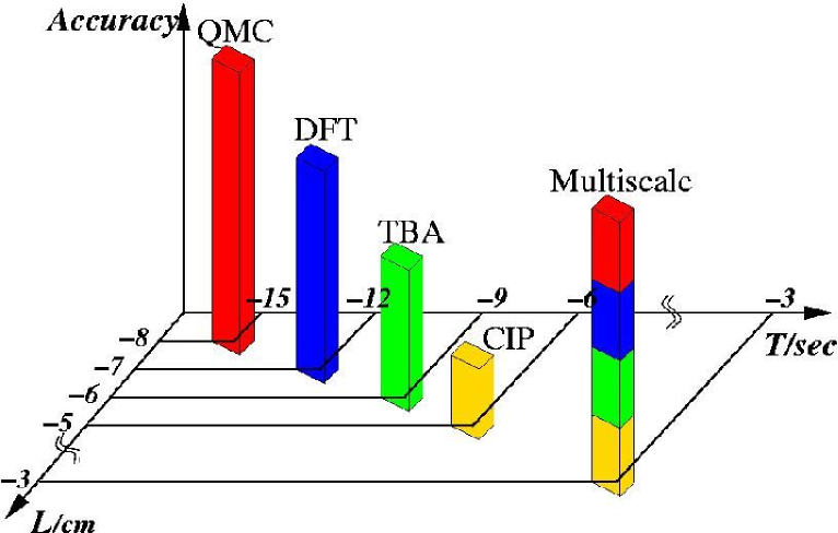
Figure 1: A schematic illustration of spacial and temporal scales achievable by various simulation approaches. The scales are in centimeters for the length dimension and seconds for the time dimension, both logarithmic.

The challenge in modern simulations of materials science and engineering is that real materials usually exhibit phenomena at one scale that require a very accurate and computationally expensive description, and phenomena at another scale for which a coarser description is satisfactory and in fact necessary to avoid prohibitively large computations. Since none of the methods above alone would suffice to describe the entire system, the goal becomes to develop models that combine different methods specialized at different scales, effectively distributing the computational power where it is needed most. It is the hope that a multiscale approach is the answer to such a quest, and it is by definition an approach that takes advantage of the multiple scales present in a material and builds a unified description by linking the models at the different scales. Fig. 1 illustrates the concept of a unified multiscale approach which can reach the length and time scale that individual methods, developed to treat a particular scale accurately, fail to achieve. At the same time, the unified approach can retain the accuracy that the individual approaches provide in their respective scales, allowing, for instance, for very high accuracy in particular regions of the systems as required. As effective theories, multiscale models are also useful for gaining physical insight that might not be apparent from brute force computations. Specifically, a multiscale model can be an effective way to facilitate the reduction and the analysis of data which sometimes can be overwhelming. Overall, the goal of multiscale approaches is to predict the performance and behavior of materials across all relevant length and time scales, striving to achieve a balance between accuracy, efficiency and realistic description.

Conceptually, two categories of multiscale simulations can be envisioned, sequential and concurrent. The sequential methodology attempts to piece together a hierarchy of computational approaches in which large-scale models use the coarse-grained representations with information obtained from more detailed, smaller-scale models. This sequential modeling approach has proven effective in systems where the different scales are weakly coupled. The characteristic of the systems that are suited for a sequential approach is that the large-scale variations decouple from the small-scale physics, or the large-scale variations appear homogeneous and quasi-static from the small-scale point of view. Sequential approaches have also been referred to as serial, implicit or message-passing methods. The vast majority of multiscale simulations that are actually in use are sequential. Examples of such approaches abound in literature, including almost all MD simulations whose underlying potentials are derived from electronic structure theory pettifor1 ; pettifor2 , usually ab initio calculations bazant ; eam . One frequently mentioned abraham1 ; abraham2 example of sequential multiscale simulations is the work of Clementi et al. clementi who used QC calculations to evaluate the interaction of several water molecules; from this database, an empirical potential was parameterized for use in molecular dynamics simulations; the MD simulations were then used to evaluate the viscosity of water from atomic autocorrelation functions; and finally, the computed viscosity was employed in computational fluid dynamics calculations to predict the tidal circulation in Buzzard’s Bay of Massachusetts.

The second category of multiscale simulations consists of the so-called concurrent, or parallel, or explicit approaches. These approaches attempt to link methods appropriate at each scale together in a combined model where the different scales of the system are considered concurrently and communicate with some type of hand-shaking procedure. This approach is necessary for systems that are inherently multiscale, that is, systems whose behavior at each scale depends strongly on what happens at the other scales. In contrast to sequential approaches, the concurrent simulations are still relatively new and only a few models have been developed to date. In a concurrent simulation, the system is often partitioned into domains characterized by different scales and physics. The challenge of the concurrent approach lies at the coupling between the different regions treated by different methods, and a successful multiscale model seeks a smooth coupling between these regions.

In principle, multiscale simulations could be based on a hybrid scheme, using elements from both the sequential and the concurrent approaches. We will not examine this type of approach in any detail, since it involves no new concepts other than the successful combination of elements underlying the other two types of approaches.

There already exist a few review papers and special editions of articles on multiscale simulation of materials in literature kaxiras ; mrs ; bullard ; ghoniem ; robertson ; kubin2 ; campbell . A mathematic perspective of multiscale modeling and computation is also available weinan_ams . The present overview does not aim to provide another collection of various multiscale techniques, but rather to identify the characteristic features and classify multiscale simulation approaches into rational categories in relation to the problems where they apply. We select a few illustrative examples for each category and try to establish connections between these approaches whenever possible. Since almost all interesting material behavior and processes are time dependent, we will address both the issue of length-scales and the issue of time-scales integration in materials modeling.

The paper is organized as follows: In Section II we discuss in detail representative examples of sequential multiscale approaches in the spatial regime. In Section III we present examples of concurrent multiscale approaches, also in the spatial regime . In Section IV we discuss representative approaches that extend time-scales in dynamical simulations. Section V contains our comments and conclusions for the applicability of the various approaches. The examples presented in this overview to some extent reflect our own research interests and they are by no means exhaustive. Nevertheless, we hope that they give a satisfactory cross-section of the current state of the field, and they can serve as inspiration for further developments in this exciting endeavor.

II Sequential multiscale approaches

Two ingredients are required in order to construct a successful sequential multiscale model:
(i) It is necessary to have a priori and complete knowledge of the fundamental processes at the lowest scale involved. This knowledge or information can then be used for modeling the system at successively coarser scales.
(ii) It is necessary to have a reliable strategy for encompassing the lower-scale information into the coarser scales. This is often accomplished by phenomenological theories, which contain a few key parameters (these can be functions), the value of which is determined from the information at the lower scale.
This message-passing approach can be performed in sequence for multiple length scales, as in the example cited in the introductionclementi . The key attribute of the sequential approach is that the simulation at a higher level critically depends on the completeness and the correctness of the information gathered at the lower level, as well as the efficiency and reliability of the model at the coarser level.

To illustrate this type of approach, we will present two examples of sequential multiscale approaches in some detail. The first example concerns the modeling of dislocation properties in the context of the Peierls-Nabarro (P-N) phenomenological model, where the lower scale information is in the form of the so-called generalized stacking fault energy surface (also referred to as the $\gamma$-surface), and the coarse-grained model is a phenomenological continuum description. The second example concerns the modeling of coherent phase transformations in the context of the phase-field approach, where the lower scale knowledge is in the form of ab initio free energies, and the coarse-grained model is again a continuum model.

II.1 Peierls-Nabarro model of dislocations

Dislocations are central to our understanding of mechanical properties of crystalline solids. In particular, the creation and motion of dislocations mediate the plastic response of a crystal to external stress. While continuum elasticity theory describes well the long-range elastic strain of a dislocation for length scales beyond a few lattice spacings, it breaks down in the immediate vicinity of the dislocation core. There has been a great deal of interest in describing accurately the dislocation core structure on an atomic scale because the core structure to a large extent dictates the dislocation properties richardson ; vitek . So far, direct atomistic simulation of dislocation properties based on CIP has not been satisfactory because the CIP is not always reliable or may even not be available for the material of interest, especially when the physical system involves several types of atoms. On the other hand, ab initio calculations are still computationally expensive for the study of dislocation core properties, particularly of dislocation mobility. Recently, a promising approach based on the framework of the Peierls-Nabarro (P-N) model has attracted considerable interest for the study of dislocation core structure and mobility joos1 ; joos2 ; juan ; hartford ; sydow ; medvedeva ; mryasov ; bulatov1 ; lu1 ; lu2 ; lu3 ; lu4 . This approach when combined with ab initio calculations for the energetics, represents a plausible alternative to the direct ab initio simulations of dislocation properties.

The P-N model is an inherently multiscale framework, first proposed by Peierls peierls and Nabarro nabarro to incorporate the details of a discrete dislocation core into an essentially continuum framework. Consider a solid with an edge dislocation in the middle (Fig. 2): the solid containing this dislocation is represented by two elastic half-spaces joined by atomic level forces across their common interface, known as the glide plane (dashed line). The goal of the P-N model is to determine the slip distribution on the glide plane, which minimizes the total energy. The dislocation is characterized by the slip (relative displacement) distribution

$${\bf f}(x)={\bf u}(x,0^{+})-{\bf u}(x,0^{-})$$ (1)

which is a measure of the misfit across the glide plane; ${\bf u}(x,0^{+})$ and ${\bf u}(x,0^{-})$ are the displacement of the half-spaces at position $x$ immediately above and below the glide plane. The total energy of the dislocated solid includes two contributions: (1) the nonlinear potential energy due to the atomistic interaction across the glide plane, and (2) the elastic energy stored in the two half-spaces associated with the presence of the dislocation. Both energies are functionals of the slip distribution ${\bf f}(x)$. Specifically, the nonlinear misfit energy can be written as

$$U_{misfit}=\int^{\infty}_{-\infty}\gamma({\bf f}(x))dx,$$ (2)

where $\gamma({\bf f})$ is the generalized stacking fault energy surface (the $\gamma$-surface) introduced by Vitek vitek1 . The nonlinear interplanar $\gamma$-surface can, in general, be determined from atomistic calculations. For systems where CIP are not available or not reliable (for instance, it is exceedingly difficult to derive reliable potentials for multi-component alloys), ab initio calculations can be performed to obtain the $\gamma$-surface. On the other hand, the elastic energy of the dislocation can be calculated reasonably from elasticity theory: the dislocation may be thought of as a continuous distribution of infinitesimal dislocations whose Burgers vectors integrate to that of the original dislocation eshelby0 . Therefore, the elastic energy of the original dislocation is just the sum of the elastic energy due to all the infinitesimal dislocations (from the superposition principle of linear elasticity theory), which can be written as

$$U_{elastic}=\frac{\mu}{2\pi(1-\nu)}\int dx\int dx^{\prime}\ln\frac{L}{|x-x^{\prime}|}\frac{d{\bf f}(x)}{dx}\frac{d{\bf f}(x^{\prime})}{dx^{\prime}}$$ (3)

where $\mu$, and $\nu$ are the shear modulus and Poisson’s ratio, respectively. $L$ is an inconsequential constant introduced as a large-distance cutoff for the computation of the logarithmic interaction energy hirth . Note that the Burgers vector of each infinitesimal dislocation is the local gradient in the slip distribution, $d{\bf f}(x)/dx$. The gradient of ${\bf f}(x)$ is called dislocation (misfit) density, denoted by $\rho(x)$. Since the P-N model requires that atomistic information (embodied in the $\gamma$-surface) be incorporated into a coarse-grained continuum framework, it is a sequential multiscale strategy. Thus the successful application of the method depends on the reliability of both $\gamma$-surface and the underlying elasticity theory which is the basis for the formulation of the phenomenological theory.

In the current formulation, the total energy is a functional of misfit distribution ${\bf f}(x)$ or equivalently $\rho(x)$, and it is invariant with respect to arbitrary translation of $\rho(x)$ and ${\bf f}(x)$. In order to regain the lattice discreteness, the integration of the $\gamma$-energy in Eq. (2) was discretized and replaced by a lattice sum in the original P-N formulation,

$$U_{misfit}=\sum_{i=-\infty}^{\infty}\gamma({\bf f}_{i})\Delta x,$$ (4)

with $x_{i}$ the reference position and $\Delta x$ the average spacing of the atomic rows in the lattice. This procedure, however, is inconsistent with evaluation of elastic energy [Eq. (3)] as a continuous integral. Therefore the total energy is not variational. Furthermore in the original P-N model, the shape of the solution ${\bf f}(x)$ is assumed to be invariant during dislocation translation, a problem that is also associated with the non-variational formulation of the total energy.

To resolve these problems, a so-called Semidiscrete Variational P-N (SVPN) model was recently developedbulatov1 , which allows for the first time the study of narrow dislocations, a situation that the standard P-N model can not handle. Within this approach, the equilibrium structure of a dislocation is obtained by minimizing the dislocation energy functional

$$U_{disl}=U_{elastic}+U_{misfit}+U_{stress}+Kb^{2}lnL,$$ (5)

where

$$U_{elastic}=\sum_{i,j}\frac{1}{2}\chi_{ij}[K_{e}(\rho_{i}^{(1)}\rho_{j}^{(1)}+\rho_{i}^{(2)}\rho_{j}^{(2)})+K_{s}\rho_{i}^{(3)}\rho_{j}^{(3)}],$$ (6)

$$U_{misfit}=\sum_{i}\Delta x\gamma_{3}({\bf f}_{i}),$$ (7)

$$U_{stress}=-\sum_{i,l}\frac{x_{i}^{2}-x_{i-1}^{2}}{2}(\rho_{i}^{(l)}\tau_{i}^{(l)}),$$ (8)

with respect to the dislocation misfit density. Here, $\rho_{i}^{(1)}$, $\rho_{i}^{(2)}$ and $\rho_{i}^{(3)}$ are the edge, vertical and screw components of the general interplanar misfit density at the $i$-th nodal point, and $\gamma_{3}({\bf f}_{i})$ is the corresponding three-dimensional $\gamma$-surface. The components of the applied stress interacting with the $\rho_{i}^{(1)}$, $\rho_{i}^{(2)}$ and $\rho_{i}^{(3)}$, are $\tau^{(1)}=\sigma_{21}$, $\tau^{(2)}=\sigma_{22}$ and $\tau^{(3)}=\sigma_{23}$, respectively. $K$, $K_{e}$ and $K_{s}$ are the pre-logarithmic elastic energy factors hirth . The dislocation density at the $i$-th nodal point is $\rho_{i}=(f_{i}-f_{i-1})/(x_{i}-x_{i-1})$ and $\chi_{ij}$ is the elastic energy kernel bulatov1 .

The first term in the energy functional, $U_{elastic}$ is now discretized in order to be consistent with the discretized misfit energy, which makes the total energy functional variational. Another modification in this approach is that the nonlinear misfit potential in the energy functional, $U_{misfit}$, is a function of all three components of the nodal misfit, ${\bf f}(x_{i})$. Namely, in addition to the misfit along the Burgers vector, lateral and even vertical misfits across the glide plane are also included. This allows the treatment of straight dislocations of arbitrary orientation in arbitrary glide planes. Furthermore, because the misfit vector ${\bf f}(x_{i})$ is allowed to change during the process of dislocation translation, the energy barrier (referred to as the Peierls barrier) can be significantly lowered compared to its corresponding value from a rigid translation. The response of a dislocation to an applied stress is achieved by minimization of the energy functional with respect to $\rho_{i}$ at the given value of the applied stress, $\tau_{i}^{(l)}$. An instability is reached when an optimal solution for $\rho_{i}$ no longer exists, which is manifested numerically by the failure of the minimization procedure to converge. The Peierls stress is defined as the critical value of the applied stress which gives rise to this instability.

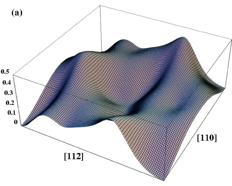
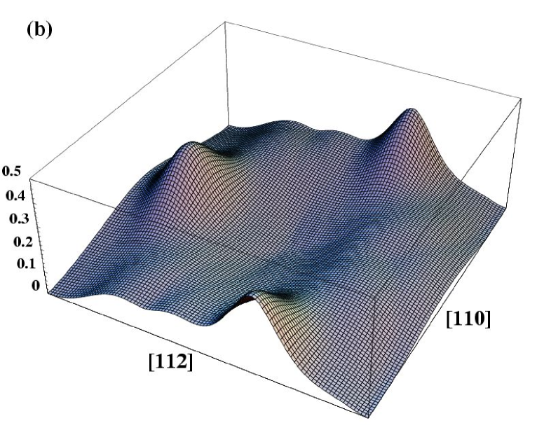
Figure 3: The $\gamma$-surface (J/m²) for displacements along a (111) plane for (a) pure Al and (b) Al+H systems. The corners of the plane and its center correspond to identical equilibrium configurations, i.e., the ideal lattice. The two surfaces are displayed in exactly the same perspective and on the same energy scale to facilitate comparison of important features.

The SVPN model has been applied to study various interesting material problems related to dislocation phenomena lu2 ; lu3 ; lu4 . One study involved the understanding of hydrogen-enhanced local plasticity (HELP) in Al. HELP is regarded as one of three general mechanisms responsible for H embrittlement of metals help . There has been overwhelming experimental evidence in support of HELP, but a theoretical foundation was lacking. In order to gain understanding of the physics behind the HELP mechanism, Lu et al. carried out ab initio calculations for the $\gamma$-surface of Al with H impurities placed at the interstitial sites lu2 . The $\gamma$-surface for both pure Al and the Al+H systems is shown in Fig. 3. Comparing the two $\gamma$-surfaces, one finds an overall reduction in $\gamma$ energy in the presence of H, which is attributed to the change of atomic bonding across the glide plane, from covalent-like to ionic-like daniel .

The core properties of four different dislocations, screw (0^∘), 30^∘, 60^∘ and edge (90^∘) have been studied using the SVPN model combined with the ab initio determined $\gamma$-surface. It was found that the Peierls stress for these dislocations is reduced by more than an order of magnitude in the presence of H lu2 , which is compatible with the experimental findings that support the HELP mechanismhelp . Moreover, in order to address the experimental observation for H trapping at dislocation cores and H-induced slip planarity, the H binding energy to the dislocation cores was calculatedlu2 . These calculations showed that there is strong binding between H and dislocation cores, that is, H is attracted (trapped) to dislocation cores which lowers the core energies. More importantly, the binding energy was found to be a function of dislocation character, with the edge dislocation having the greatest and the screw dislocation having the lowest binding energy. For a mixed dislocation, the binding energy increases with the amount of edge component of the Burgers vector. These results suggest that in the presence of H, it costs more energy for an edge dislocation to transform into a screw dislocation in order to cross-slip, since the edge dislocation has almost twice the binding energy of the screw dislocation lu2 . In the same vein, it costs more energy for a mixed dislocation to transfer its edge component to a screw component for cross-slip. Therefore the cross-slip process is suppressed due to the presence of H, and slip is confined to the primary glide plane, exhibiting the experimentally observed slip planarity.

A similar approach was applied to the study of the vacancy lubrication effect on dislocation motion in Al. From this analysis, it was shown that the role of vacancies is crucial in reconciling the results of Peierls stress measured from different experimental techniques lu3 . Very recently, a multiple plane P-N model has been developed to study dislocation phenomena involving more than one glide planes, such as dislocation constriction and cross-slip lu4 . Finally we should point out that the P-N model is just one example of more general cohesive surface models that are built upon the idea of limiting all constitutive nonlinearity to certain privileged interfaces, while the remainder of the material is treated via more conventional continuum theories rob . The same strategy can also be applied to the study of fracture and dislocation nucleation from a crack tip guanshui .

It is interesting to note that the analysis of $\gamma$-surface can provide a qualitative understanding of even more complex mechanical properties of materials. For example, Rice and coworkers Rice formulated powerful criteria for the brittle behavior of materials, by extending the Peierls analysis to geometries involving cracks. Based on this framework, Waghmare et al.umesh1 ; umesh2 were able to predict which alloying elements could improve the ductility of MoSi₂ by analyzing the ab initio determined $\gamma$-surface of the alloys, and comparing the changes induced by alloying to key features of the $\gamma$-surface versus the changes induced to the surface energy $\gamma_{s}$. Remarkably, certain predictions of this relatively simple theoretical modeling were borne out by subsequent experiments peralta .

We have devoted some attention to the description of the P-N model and its implementation using ab initio $\gamma$-surfaces, because it is an ideal case of a sequential multiscale model: it consists of a well motivated phenomenological framework, within which the set of atomistically derived quantities is well defined and complete (in this case the $\gamma$-surface). In this sense, it fulfills all the requirements for a coherent and complete multiscale model. There are no doubt limitations to it, arising from the range of validity of the phenomenological theory, but within this range there are no other ambiguities in constructing the multiscale model. Perhaps, its successes, some of which we presented above, are owed to this complete character of the model.

II.2 Phase-field model of coherent phase transformations

The structure-properties paradigm is one of the principal pillars in materials science. The term “structure” here refers to structures at many different scales, including the atomic scale geometry determined by the crystalline arrangement of atoms, the structure of the defects that exist in a material, and the structure that emerges as a result of the organization of these defects into what is referred to as microstructure. Among these structures, the microstructure on the scale of micrometers is often directly tied to the mechanical properties of materials, and has therefore attracted great interest both in terms of scientific understanding and practical applications suo ; cocks ; gurtin ; bullard1 ; fan .

Recently, a powerful sequential multiscale approach has been put forward for modeling the precipitate microstructure and its evolution in multicomponent alloys chen1 ; vaith , materials which appear in many technological applications. The approach is based on the continuum phase-field model whose driving forces (free energies) are obtained from combined ab initio calculations and the mixed-space cluster expansion technique. One interesting application of this approach concerned the study of precipitation of the $\theta^{\prime}$(Al₂Cu) phase in Cu-Al alloys during thermal aging vaith .

In the phase-field multiscale approach, the nature of phase transformation as well as the microstructures that are produced are described by a set of continuous order-parameter fields wang ; chen2 . The temporal microstructure evolution is obtained from solving field kinetic equations that govern the time-dependence of the spatially inhomogeneous order-parameter fields. Within the diffuse-interface description, the thermodynamics of a phase transformation and the accompanying microstructure evolution are modeled by a free energy that is a function of the order-parameter field, or phase field. For a structural transformation, the total free energy can be written as:

$${\cal F}_{tot}={\cal F}_{bulk}+{\cal F}_{inter}+{\cal F}_{elast}$$ (9)

where ${\cal F}_{bulk}$ is the bulk free energy, ${\cal F}_{inter}$ is the interfacial free energy, and ${\cal F}_{elast}$ is the coherency elastic strain energy arising from the lattice accommodation along the coherent interfaces in a microstructure. For a microstructure described by a composition field $c$ and a set of structural order-parameters, $\eta_{1}$, …, $\eta_{p}$, the first two terms of Eq. (9) are given by

$${\cal F}_{bulk}+{\cal F}_{inter} = \int_{V}\{f[c({\bf r}),\eta_{p}({\bf r})]+\frac{\alpha}{2}|\nabla c({\bf r})|^{2}$$

$$+\frac{1}{2}\sum\limits_{p}\beta_{ij}(p)\nabla_{i}\eta_{p}({\bf r})\nabla_{j}\eta_{p}({\bf r})\}dV$$

where $f(c,\eta_{p})$ is the local free energy density li and $\alpha$ and $\beta_{ij}(p)$ are the gradient energy coefficients which control the width of the diffuse interface. The elastic strain energy is obtained from elasticity theory using the homogeneous modulus approximation khach . With the total free energy of an inhomogeneous system written as a function of order-parameter fields, the temporal evolution of microstructures during a phase transformation can be obtained by solving the coupled Cahn-Hilliard equation for a conserved field $c$, and the time-dependent Ginzburg-Landau equation for a non-conserved field $\eta_{p}$ cahn ; hohenberg :

$$\frac{\partial c}{\partial t}=M\nabla^{2}\left[\frac{\partial f}{\partial c}-\alpha\nabla^{2}c\right]$$ (11)

$$\frac{\partial\eta_{p}}{\partial t}=-L_{p}\frac{\delta{\cal F}_{tot}}{\delta\eta_{p}}$$ (12)

where $M$ is related to atom mobility and $L_{p}$ is the relaxation constant associated with the order-parameter $\eta_{p}$. As the above equations illustrate, the continuum phase-field methodology depends on three input energies: (1) bulk free energies of solid solution and precipitate phases, (2) precipitate-matrix interfacial free energies, and (3) precipitate/matrix lattice elastic energies. Experimental determination of these quantities can be difficult and problematic. Therefore a physically motivated method for accurately determining these quantities is of critical importance to predict the microstructure evolution of interest. In particular, if the quantities can be determined from ab initio calculations, the goal of an “ab initio” modeling of alloy microstructure evolution would be, to a great extent, achieved zunger0 ; defontaine .

Since direct ab initio calculations of free energies are either impractical or impossible with currently available computational power, a useful method has been developed to extend the ab initio energetics to thermodynamic properties of alloy systems with hundreds of thousands of atoms wolv , referred to as the mixed-space cluster expansion (CE). In this scheme, energetics from ab initio calculations for a number of small unit cell ($\sim$ 10 atoms) structures are mapped onto a generalized Ising-like model for a particular lattice type, involving 2-, 3-, and 4-body interactions plus coherency strain energies zunger . The Hamiltonian can be incorporated into mixed-space Monte Carlo simulations of $N\sim 10^{5}$ atoms, effectively allowing one to explore the complexity of $2^{N}$ configurational space. As demonstrated by Vaithyanathan et al., the bulk free energy can be obtained from Monte Carlo simulations coupled with thermodynamic integration techniques. The precipitate/matrix interfacial free energies can be determined from similar Monte Carlo simulations or from low temperature expansion techniques. The elastic strain energies are of precisely the same form as the coherency strain energy used to generate the mixed-space CE. Hence, from a combination of ab initio calculations, a mixed-space CE approach, and Monte Carlo simulations, one can obtain all the driving forces needed as input to the continuum phase-field model. The incorporation of these energetic properties, obtained from atomistics, into a continuum microstructural model represents a bridge between these two length scales, and opens the path toward predictive modeling of microstructures and their evolution.

To illustrate the use of the method, we mention briefly the work of Vaithyanathan et al. who studied the problem of precipitation of the $\theta^{\prime}$ (Al₂Cu) phase in Cu-Al alloys. The free energy of the $\theta^{\prime}$ phase is obtained from ab initio calculations of the energy at $T=0$ K, coupled with the calculated vibrational entropy of this phase. The bulk free energies of matrix and precipitate phases are then fit to the local free energy as a function of order-parameter fields in the phase-field model. $T=0$ K interfacial energies are determined from supercell calculations, both for the coherent interface and for the incoherent interface. The anisotropy of these interfacial energies is large and has been incorporated in the phase-field model. Elastic energy calculations for the coherent strain of Al/Al₂Cu ($\theta^{\prime}$) and the calculated lattice parameters of each phase determine the elastic driving force in this system. Having determined all the necessary thermodynamic input, Vaithyanathan et al. were able, for the first time, to clarify the physical contributions responsible for the observed morphology of $\theta^{\prime}$ precipitate microstructure. The agreement between the calculated and experimentally observed microstructure of $\theta^{\prime}$ in the Al-Cu alloys was excellent, confirming the validity of the approach.

Although the phase-field model is able to predict complex microstructure evolution during phase transformations, it requires as input phenomenological thermodynamic and kinetic parameters. For binary systems, ab initio calculations can provide these parameters for the phase-field model, but it is unrealistic to assume that such calculations can be used to determine all the thermodynamic information for systems beyond ternary. Therefore semi-empirical methods, such as CALPHAD (calculated phase-diagram) will remain a useful tool in such an endeavor kaufman ; saunders ; spencer .

II.3 Other sequential approaches

Kinetic Monte Carlo (KMC) simulations, coupled with atomistically determined kinetic energy barriers, represent a powerful class of sequential multiscale approaches. For example, a large body of research has been carried out for surface growth phenomena with KMC simulations whose kinetic energy barrier parameters for relevant elemental processes are supplied by ab initio calculations kandel ; scheffler . In an altogether different field, Cai et al. have used KMC method to study dislocation motion in Si based on the well-established double-kink mechanism cai . In their approach, the dislocation is represented by a connected set of straight line segments which move as the cumulative effect of a large number of kink nucleation and migration processes. The rate of these processes is calculated from transition state theory with the transition energy barrier having contributions from both atomistically determined energetics (double-kink formation and migration energy) and elastic interactions with other dislocation segments as well as from the externally applied stress.

An example of a multiscale approach, in which KMC is a key component, employs the so-called level-set method ratsch ; gyure for the largest (macroscopic) scale. This approach is particularly well suited for the study of epitaxial growth, a subject of great importance in microelectronics and optoelectronics applications. In the level-set method, growth is described by creation and subsequent motion of island boundaries. The model treats the growing film as a continuum in the lateral direction, but retains atomistic discreteness in the growth direction. In the lateral direction, continuum equations representing the field variables can be coupled to growth through island evolution, by solving the appropriate boundary-value problem for the field and using local values of this field to determine the velocity of the island boundaries. The central idea behind the level-set method osher is that any boundary curve $\Gamma$, such as a step or the boundary of an island, can be represented as the set of values $\varphi=0$ (the level-set) of a smooth function $\varphi$. For a given boundary velocity $v$, the equation for $\varphi$ is

$$\frac{\partial\varphi}{\partial t}+{\bf v}\cdot\nabla\varphi=0$$ (13)

Growth is naturally described by the smooth evolution of $\varphi$ determined by this differential equation. In the case of multilayer growth, the boundaries $\Gamma_{k}(t)$ of the islands are defined as the set of spatial points $x$ for which $\varphi({\bf x},t)=k$ for $k=0,1,2,\dots$. The evolution of the level-set function $\varphi$ can be obtained by numerically solving Eq. (13) using non-oscillatory methods shu . The key parameters entering the model are diffusion constants (the terrace and island-edge diffusion constants) which can in principle be supplied from atomistic calculations, through the following procedure (see Fig. 4): first, the atomistic processes are identified which are responsible for terrace or island-edge diffusion and their energetics are analyzed using atomistic (possibly ab initio) calculations; next, the energy barriers for the atomistic processes are incorporated in a KMC model which provides the means for coarse-graining the atomistic degrees of freedom to a few mesoscopic degrees of freedom describing the evolution of surface features (the island step edges); finally, the results of the KMC model are coarse-grained to provide the input to the level-set equations, that is, they define the values of the boundary velocity v which depends on the local surface morphology. The coarse-graining between scales eliminates degrees of freedom that are not essential, making the passage to the next scale feasible. For example, in the illustration shown in Fig. 4, the smallest step width in the KMC scale corresponds to a two-atom wide region at the microscopic scale, a situation that is relevant to the Si(100) surface and possibly to other semiconductor surfaces (such as III-V compound surfaces). In these cases, surface atoms tend to be bound to dimer pairs, which is the essential unit that determines the step structure, even though the underlying dynamics may be determined by the motion of individual atoms. Thus, the KMC simulation need only take into account structures consisting of dimer units, the dynamics of which determine the step-edge motion needed for the level-set simulation. The middle terrace in Fig. 4(b) is shown as a grid of squares, each representing a four-atom cluster and being the minimal unit relevant to step motion at the KMC scale in this example, assuming that only steps of width equal to two atoms in each direction are stable. The level-set method is a manifestly multiscale approach, combining information from three different regimes (atomistic, mesoscopic and continuum) into a neatly integrated scheme. Recently, the level-set method has also been applied to study dislocation dynamics in alloys srolovitz .

Yet another sequential multiscale approach has been successfully applied to the study of crystal plasticity. This is the DD method mentioned earlier, incorporating dislocation motion at the macroscopic scale, the mechanism ultimately responsible for crystal plasticity. In order to predict the mechanical properties of materials using DD simulations, a connection between micro-to-meso scales must be established because dislocation interactions at close range (when the cores intersect, for instance), are totally beyond the reach of continuum models. Along these lines, Bulatov et al. were able to study dislocation reactions and plasticity in fcc metals vasily2 that compare well with deformation experiments, by integrating the local rules derived from atomistic simulation of dislocation core interactions into the DD simulations. The same idea has been further explored by Rhee et al. in a study of the stage I stress-strain behavior of bcc single crystals rhee .

III Concurrent multiscale approaches

Broadly speaking, a concurrent multiscale approach is more general in scope than its sequential counterpart because the concurrent approach does not rely on any assumptions (in the form of a particular coarse-graining model) pertaining to a particular physical problem. As a consequence, a successful concurrent approach can be used to study many different problems. For example, dislocation core properties, grain boundary structure and crack propagation could all be modeled individually or collectively by the same concurrent approach, as long as it incorporates all the relevant features at each level. What is probably most appealing, however, is that a concurrent approach does not require a priori knowledge of the physical quantities or processes of interest. Thus, concurrent approaches are particularly useful to explore problems about which little is known at the atomistic level and its connection to larger scales, and to discover new phenomena. We discuss below three instances of concurrent approaches in some detail, and mention some additional examples more briefly.

III.1 Macroscopic Atomistic Ab initio Dynamics

Fracture dynamics is one of the most challenging problems in materials science and solid mechanics. Despite nearly a century of study, several important issues remain unsolved. In particular, there is little fundamental understanding of the brittle to ductile transition as a function of temperature in materials; there is still no definitive explanation of how fracture stress is transmitted through plastic zones at crack tips; and there is no complete understanding of the disagreement between theory and experiment regarding the limiting speed of crack propagation. These difficulties stem from the fact that fracture phenomena are governed by processes occurring over a wide range of length scales that are all connected, and all contribute to the total fracture energy needleman2 . In particular, the physics on different length scales interacts dynamically, therefore a sequential coupling scheme would not be adequate for the study of fracture dynamics.

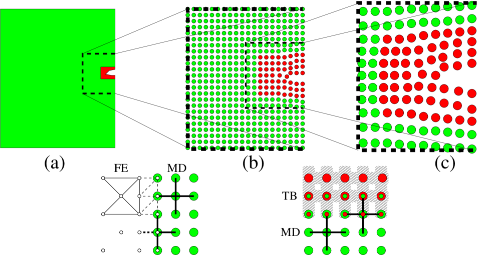
Figure 5: Geometrical decomposition of a Si slab with a small crack into different dynamic regions in the a MAAD simulation: (a) The system at the macroscopic scale, which is modeled as a continuum using finite elements (FE), except for the region near the crack outlined in dashed line. (b) The mesoscopic scale, treated atomistically with interatomic potentials and molecular dynamics (MD) with the atoms indicated by green circles, except for the region in the immediate neighborhood of the crack, outlined in dashed line. (c) The microcopic scale, treated atomistically with forces derived from quantum mechanical calculations with the atoms indicated by red circles. The hand shaking regions between FE and MD and between MD and TB are also shown schematically (see text for details).

To address these challenges, Abraham, Broughton, Bernstein and Kaxiras developed a concurrent multiscale modeling approach that dynamically couples different length scales abraham1 ; abraham2 . This multiscale methodology aims at linking the length scales ranging from the atomic scale, treated with a quantum-mechanical tight-binding approximation method, through the microscale, treated via the classical molecular dynamics method, and finally to the mesoscale/macroscale treated via the finite element method in the context of continuum elasticity. These authors applied this unified approach, termed macroscopic-atomistic-ab initio dynamics (MAAD), to the study of the dynamical fracture process in Si, a typical brittle material. In traditional studies of fracture, only the continuum mechanics level (employing, for instance, the FE method) is usually invoked to account for the macroscopic behavior. But since there is no natural small-length cutoff present in the continuum mechanics approach, any important aspect of the atomic-scale mechanisms for fracture is completely missed. This can be remedied by introducing classical MD to the simulations. In particular, the MAAD approach employed the Stillinger-Weber sw interatomic empirical potential for Si to perform MD calculations at the atomistic level, for a large region of the material near a crack tip. However, the treatment of formation and breaking of covalent bonds at the atomic scale is not reliable with any empirical potential, because bonds between atoms are an essentially quantum mechanical phenomenon arising from the sharing of valence electrons. On the other hand, small deviations from ideal bonding arrangements can be captured accurately by empirical potentials, because they are to first approximation harmonic, a feature that is easily incorporated in empirical descriptions of the interaction between atoms. Therefore, it was deemed necessary to include a quantum mechanical approach into the simulations for a small region in the immediate neighborhood of the crack tip, where bond breaking is prevalent during fracture, while further away from this region the empirical potential description is adequate. The particular methodology chosen to model the immediate neighborhood of the crack-tip, a semi-empirical nonorthogonal tight-binding scheme tb , describes well the bulk, amorphous, and surfaces properties of Si. Fig. 5 shows the spatial decomposition of the computational cell into five different dynamic regions of the simulation: the continuum FE region at the far-field where the atomic displacements and strain gradients are small; the atomistic MD region around the crack with large strain gradients but with no bond breaking; the quantum mechanical region (labelled TB because of the use of the tight-binding method) right at the crack tip where atomic bonds are being broken and formed; the FE/MD hand-shaking region; and the MD/TB hand-shaking region. The total Hamiltonian, $H_{tot}$ for the entire system was written as:

$$H_{tot} = H_{FE}(\{{\bf u,\dot{u}}\}\in FE)+$$

$$H_{MD}(\{{\bf r,\dot{r}}\}\in MD)+$$

$$H_{TB}(\{{\bf r,\dot{r}}\}\in TB)+$$

$$H_{FE/MD}(\{{\bf u,\dot{u},r,\dot{r}}\}\in FE/MD)+$$

$$H_{MD/TB}(\{{\bf r,\dot{r}}\}\in MD/TB)$$

The degrees of freedom of the Hamiltonian are atomic positions r and velocities $\dot{\bf r}$ for the TB and MD regions, and displacements u and their time rates of change $\dot{\bf u}$ for the FE regions. Equations of motion for all the relevant variables in the system are obtained by taking appropriate derivatives of this Hamiltonian. All variables can then be updated in lock-step as a function of time using the same integrator. Thus the entire time history of the system may be obtained numerically given an appropriate set of initial conditions. Following trajectories dictated by this Hamiltonian leads to evolution of the system with conserved total energy, which ensures numerical stability.

The individual approaches at each level (FE, MD and TB) are well established and tested methods. What was much more important in this study was the seamless hand-shaking of the different methods at the interface of the respective domains, namely the hand-shaking algorithms between FE and MD regions and between the MD and TB regions. We present here the main ideas behind the coupling of the different regions.
FE/MD coupling: To achieve the FE/MD hand-shaking, the FE mesh spacing is scaled down to atomic dimensions at the interface of the two regions. In Fig. 5, the FE nodes are indicated as small open circles connected by thin lines. Moving away from the FE/MD region and deep into the continuum, one can expand the mesh size. In this way, the atomistic simulation is embedded in a large continuum solid, indicated by a green-colored region in Fig. 5(a). FE cells contributing fully to the overall Hamiltonian (unit weight) are marked with thin solid lines, while cells contributing to the hand-shake Hamiltonian (half weight) are represented by thin dashed lines. Interactions between the atoms on the MD side, which are represented by an interatomic potential, carry full weight when fully inside the MD region (thick solid lines joining neighboring atoms) and half weight (thick dashed lines) when they cross the boundary, with one of the neighbors effectively represented by a node in the FE region. The FE/MD interface is chosen to be far from the fracture region. Hence, the atoms of the MD region and the displacements of the FE lattice can be unambiguously mapped onto one another. The assignment of weights equal to unity within each region and equal to one half at the interface is arbitrary and can be generalized by the introduction of a smooth step function.
MD/TB coupling: At this interface, the atoms treated quantum mechanically are shown in red while those treated classically are shown in green. The dangling bonds at the edge of the TB region are terminated with pseudo-hydrogen atoms. The Hamiltonian matrix elements of these pseudo-hydrogen atoms are carefully constructed to tie off a single Si bond and to ensure the absence of any charge transfer when that atom is placed in a position commensurate with the Si lattice. In other words, the TB terminating atoms are fictitious monovalent atoms forming covalent bonds with the strength and length of bulk Si bonds. These fictitious atoms were called “silogens”: they behave mechanically just like Si, but chemically like H. The TB Hamiltonian including silicon-silicon and silicon-silogen matrix elements is then diagonalized to obtain electronic energies and wavefunctions, from which the total energy can be computed. Thus, at the perimeter of the MD/TB region, there are silogens sitting directly on top of the atoms of the MD region, which are shown as the smaller red circles on top of green circles in Fig. 5. On one side of the TB/MD interface, the bonds to an atom are derived from the TB Hamiltonian, and are shown as shaded regions in Fig. 5, to indicate the electronic distribution responsible for the formation of the covalent bonds. On the other side of the interface, the bonds are derived from the interatomic potential of the MD simulation. The MD atoms of the interface have a full complement of neighbors, including neighbors whose positions are determined by the dynamics of atoms in the TB region; these are shown as small green circles on top of the red circles in Fig. 5. As before, the TB code updates atomic positions in lock-step with its FE and MD counterparts.

The MAAD approach was employed to study the brittle fracture of Si in a geometry containing a small crack (notch) within an otherwise perfect solid, with the exposed notch face in the (100) plane and the notch pointed in the $\langle$010$\rangle$ direction. The system consisted of 258,048 mesh points in each FE region, 1,032,192 atoms in the MD region, and approximately 280 unique atoms in the TB region (for computational reasons, the entire region modeled by the TB method was broken into smaller, partially overlapping regions, each assigned to a different processor in a parallel implementation). The lengths of the MD region are 10.9 Å  for the slab thickness along the front of the crack, 3649 Å  in the primary direction of propagation, and 521 Å  in the direction of pull (before pulling). Periodic boundary conditions were imposed at the slab faces normal to the direction of the crack propagation (along the front of the crack). The wall-clock time for a TB force update was 1.5 s, that for the MD update was 1.8 s, and that for the FE update was 0.7 s. The TB region was relocated after every 10 time steps to ensure that it remains at the very tip of the propagating crack. The computational slab was initialized at zero temperature, and a constant strain rate was imposed on the outermost FE boundaries defining the opposing horizontal faces of the slab. Furthermore, a linear velocity gradient was applied within the slab, which results in an increasing internal strain with time. It was observed that the Si solid failed in brittle fashion at the notch tip when the material is stretched by $\sim$ 1.5%. The limiting speed of crack propagation was found to be 85% of the Rayleigh speed with the chosen computational setup. In the course of the simulation, the straight-ahead brittle cleavage of the Si slab left behind a rough surface, with increasing roughening as a function of crack distance. Based on these results, the authors suggested that the roughening surface is due to the spawning of dislocations with low mobility on the time-scale of the crack motion.

A general problem associated with domain decomposition, as in the MAAD simulations, is the spurious reflection of elastic waves (phonons) at the domain boundaries due to the changes in system description across the boundaries. For example, such effects have been observed in the atomistic modeling of dislocation motion ohsawa , crack propagation gao ; zhou ; holian ; gumbsch , and energetic particle-solid collisions carroll ; moseler , all of which involved some domain coupling scheme. Since the MAAD method involves domain decomposition into the TB, MD and FE regions, the quality of coupling between different regions needs to be examined. In a subsequent paper, the same authors reported that there was no visible reflection of phonons at the FE/MD interface, and no obvious discontinuities at the MD/TB interface abraham2 . Thus, in this scheme the coupling between the various domains is indeed performed in a seamless manner, closely mimicking the actual behavior of the physical system under investigation. Overall, the MAAD approach represents the state of the art of current multiscale simulation strategies. It is a finite-temperature, dynamic and parallel algorithm which, at least as far as general computational aspects are concerned, is applicable to any type of material.

Ongoing efforts are exploring the possibility of applying the MAAD strategy to study chemical effects on mechanical properties of metallic alloys, such as impurity effects on dislocation motion, crack nucleation and propagation in various metals. There is an important qualitative difference between such systems and the study of brittle fracture of Si mentioned above: the nature of bonds in metallic systems is very different from the simple covalent bonds in Si. This makes necessary the development of a different way of coupling the quantum mechanical to the classical atomistic region, because it is no longer feasible to terminate the bonds at the boundary of the quantum region by simply saturating them with fictitious atoms like the silogens. In such endeavors, other more efficient and versatile quantum mechanical formulations are desirable. One candidate is the linear scaling real-space kinetic energy functional method choly . This method approximates the non-interacting kinetic energy of DFT as a functional of electron density, and electronic wave-functions are thus eliminated from calculations, and therefore the method is termed as orbital-free density functional theory (OFDFT). As a consequence, no diagonalization of the electronic Hamiltonian and no sampling of reciprocal space are necessary, making the method computationally efficient carter . In particular, the explicit real-space feature of this approach makes it naturally suitable for domain coupling within the MAAD framework. While efforts to construct a fully functioning scheme along these lines are continuing, we believe this is a promising method with great potential for applications in metallic systems, which are difficult to handle with other techniques.

III.2 Quasicontinuum model

One observation from many large-scale atomistic simulations is that only a small subset of atomic degrees of freedom do anything interesting. The great majority of the atoms behave in a way that could be described by effective continuum models like elasticity theory. The computation and storage of the uninteresting degrees of freedom - necessary for a fully atomistic calculation - consume a large proportion of computational resources. This observation calls for novel multiscale approaches which can reduce the number of degrees of freedom in atomic simulations kohlhoff ; gumbsch2 . One such approach proposed by Tadmor, Ortiz and Phillips is particularly promising and has yielded considerable success in many applications tadmor1 . This concurrent multiscale approach is called the quasicontinuum method, which seamlessly couples the atomistic and continuum realms. The chief objective of the approach is to systematically coarsen the atomistic description by the judicious introduction of kinematic constraints. These kinematic constraints are selected and designed so as to preserve full atomistic resolution where required - for example, in the vicinity of lattice defects - and to treat collectively large numbers of atoms in regions where the deformation field varies slowly on the scale of the lattice. Variants of the quasicontinuum model have been developed and applied in different situations tadmor1 ; tadmor2 ; shenoy1 ; miller1 ; miller2 ; rodney ; shenoy2 ; tadmor3 ; shenoy3 ; smith1 ; knap ; smith2 . The essential building blocks of the static quasicontinuum model are: (1) the constrained minimization of the atomistic energy of the solid; (2) the use of summation rules to compute the effective equilibrium equations; and (3) the use of adaptation criteria in order to tailor the computational mesh to the structure of the deformation field. An extension of the method to finite-temperature has also been proposed shenoy4 .

The quasicontinuum model starts from a conventional atomistic description, which computes the energy of the solid as a function of the atomic positions. The configuration space of the solid is then reduced to a subset of representative atoms. The positions of the remaining atoms are obtained by piecewise linear interpolations of the representative atom coordinates, much in the same manner as displacement fields are constructed in the FE method. The effective equilibrium equations are then obtained by minimizing the potential energy of the solid over the reduced configuration space. A direct calculation of the total energy in principle requires the evaluation of sums that are extended over the full collection of atoms, namely,

$$E_{tot}=\sum_{i=1}^{N}E_{i},$$ (14)

where $N$ is the total number of atoms in the solid. The full sums may be avoided by the introduction of approximate summation rules. For example, the lattice quadrature analog of Eq. (14) can be written as

$$E_{tot}\approx\sum_{i=1}^{N_{r}}n_{i}\bar{E}_{i},$$ (15)

where $n_{i}$ is the quadrature weight that signifies how many atoms a given representative atom stands for in the description of the total energy, and $\bar{E}_{i}$ is the energy of $i$-th representative atom. Note that in this case the sum is over the $N_{r}$ representative atoms only. In the quasicontinuum approach, the FE method serves as the numerical tool for determining the displacement fields, while an atomistic calculation is used to determine the energy of a given displacement field. The positions of the coarse-grained atoms are needed because the energy of the representative atoms depends on them. This approach is in contrast to standard FE schemes, where the constitutive law is introduced through a phenomenological model. The selection of the representative atoms may be based on the local variation of the deformation field. For example, near dislocation cores and on planes undergoing slip, full atomistic resolution is attained with adapted meshing. Far from defects or other highly stressed regions, the density of representative atoms rapidly decreases, and the collective motion of very large numbers of atoms is dictated, without appreciable loss of accuracy, by a small number of representative atoms.

The quasicontinuum method has been applied to a variety of problems, including dislocation structures tadmor1 ; tadmor2 , interactions of cracks with grain boundaries shenoy1 , nanoindentations tadmor3 ; smith1 ; smith2 , dislocation junctions rodney , atomistic scale fracture process miller1 , etc. By way of example, Shenoy et al. applied the method to study the interaction of dislocations with grain boundaries (GB) in Al shenoy1 . In particular, they considered a reformulation of the quasicontinuum model that allows for the treatment of interfaces, and therefore of polycrystalline solids. As the first test of the model, they computed the GB energy and atomic structure for various symmetric tilt GB’s in Au, Al, and Cu using both direct atomistic calculations and the model calculations. They found excellent agreement between the two sets of calculations, indicating the reliability of the model for their purpose. In the study of Al, they used nanoindentation-induced dislocations to probe the interaction between dislocations and GB’s. Specifically, they considered a block oriented so that the (111) planes are positioned to allow for the emergence of dislocations which then travel to the $\Sigma$ 21($\bar{2}$41) GB located at $\sim$ 200 Å  beneath the surface [see Fig. 6(a)]. First, the energy minimization is performed to obtain the equilibrium configuration of the GB, then a mesh is constructed accordingly as shown in Fig. 6(a). The region that is expected to participate in the dislocation-GB interaction is meshed with full atomistic resolution, while in the far fields the mesh is coarser. The displacement boundary conditions at the indentation surface are then imposed onto this model structure, and after the critical displacement level is reached, dislocations are nucleated at the surface. With the EAM potential eam supplying the atomistic energies in the quasicontinuum approach, they observed closely spaced (15 Å) Shockley partials nucleated at the free surface. As seen from Fig. 6(b), the partials are subsequently absorbed at the GB with the creation of a step at the GB and no evidence of slip transmission into the adjacent grain is observed. The resultant structure can be understood based on the concept of displacement shift complete lattice dsc associated with this symmetric tilt GB. As the load is increased, the second pair of Shockley partials is nucleated. These partials are not immediately absorbed into the GB, but instead form a pile-up [Fig. 6(b)]. The dislocations are not absorbed until a much higher load level is reached. Even after the second set of partial dislocations is absorbed at the GB, there is no evidence of slip transmission into the adjacent grain, although the GB becomes much less ordered. The authors argued that their results give hints for the general mechanism governing the absorption and transmission of dislocations at GB’s. The same work also studied the interaction between a brittle crack and a GB and observed stress-induced GB motion (the combination of GB sliding and migration). In this example, the reduction in the computational effort associated with the quasicontinuum thinning of degrees of freedom is significant. For example, the number of degrees of freedom associated with the mesh of Fig. 6(a) is about 10⁴, three orders of magnitude smaller than what would be required by a full atomistic simulation (10⁷ degrees of freedom).

Recently, the quasicontinuum model has been extended to complex Bravais lattices tadmor4 whereby more complicated materials can be handled smith2 . But because of the expression for the total energy adopted in Eq. (14), (15), the actual atomistic methods that can be implemented in the quasicontinuum model are limited to ones that can be easily cast in such a form, if one insists on having the ability to resolve the FE nodes all the way to the atomic scale. This limit is often referred to in the literature as the “non-local” regime of the quasicontinuum method. In contrast, the “local” limit refers to the case where each FE node represents a very large number of atomistic degrees of freedom, which is modeled as corresponding to an infinite solid homogeneously deformed according to the local strain at the node. In this limit, it is advantageous to employ effective Hamiltonians to compute energetics for the representative atoms. Such Hamiltonians can be constructed from ab initio calculations, and may include physics that atomistic simulations based on classical interatomic potentials (such as EAM) are not able to capture. For example, by constructing an effective Hamiltonian parametrized from ab initio calculations, Tadmor et al. were able to study polarization switching in piezoelectric material PbTiO₃ in the context of the quasicontinuum model in the local limittadmor5 . This particular Hamiltonian includes the following terms: the elastic energy of the lattice, the coupling between strain and atomic displacement, harmonic and anharmonic phonon energy contributions, the interaction of atomic displacement with the applied electric field, and the electrostatic energy. With this effective Hamiltonian, it was shown that the behavior of a large-strain ferroelectric actuator under the application of competing external stress and electric fields can be modeled successfully, reproducing, for example, all the important features of the experimental strain vs. electric field curve for the actuator. The advantage of these simulations is that they also provide insight into the microscopic mechanisms responsible for the macroscopic behavior, making possible the improvement of design of the technologically useful materials.

One pitfall of the quasicontinuum model is the so-called “ghost force” at the interface between the local region, identified with slow variation of the deformation gradient, and the nonlocal region, identified with rapid variation of the deformation gradient shenoy2 . The error arises from the discontinuity between the neighboring cells where the cell sizes are less than the range of the atomistic potential. Care must be taken to correct these “ghost forces” shenoy2 . Finally we should point out that the quasicontinuum approach also shares certain features with sequential approaches, namely, the constitutive equation for the FE nodes is drawn from atomistic calculations (akin to message passing in sequential approaches). The reason we categorize it as a concurrent multiscale approach is that the atomistic and FE calculations are performed concurrently rather than in sequence, because the range of deformations encountered in various parts of the system are not know beforehand. Moreover, some sort of domain partitioning (meshing) is involved in the quasicontinuum approach.

III.3 Coarse-grained molecular dynamics

Mesoscopic elastic systems, and in particular micro-electro-mechanical-systems (MEMS), recently have captured a great deal of attention and research interest as micro-machines and devices. However, there is serious concern regarding their mechanical integrity and stability in applications because these sub-micron devices are so minuscule that structural defects and surface effects could have large impact on their performance. On the other hand, the computational study of the mechanical properties of the MEMS has turned out to be extremely difficult because they are too small in size for finite-element simulations (at the limit where continuum elasticity theory may be no longer valid), but too large for atomistic simulations rudd ; rudd1 . To resolve this problem, a concurrent multiscale simulation strategy called coarse-grained molecular dynamics (CGMD) has been developed by Rudd and Broughton rudd ; rudd1 . This approach bears some resemblance with the quasicontinuum model, yet there exist important differences between the two.

The CGMD approach is based on a statistical coarse-graining prescription. In particular, the model aims at constructing scale-dependent constitutive equations for different regions in a material. In general, the material of interest can be partitioned into cells, whose size varies so that in important regions a mesh node is assigned to each equilibrium atomic position, whereas in other regions the cells contain many atoms and the nodes need not coincide with atomic sites. The CGMD approach produces equations of motion for a mean displacement field defined at the nodes by defining a conserved energy functional for the coarse-grained system as a constrained ensemble average of the atomistic energy under fixed thermodynamic conditions. The key point of this effective model is that the equations of motion for the nodal (mean) fields are not derived from the continuum model, but from the underlying atomistic model. The nodal fields represent the average properties of the corresponding atoms, and equations of motion (in this particular case Hamilton’s equations) are constructed to describe the mean behavior of underlying atoms that have been integrated out.

One important underlying principle of CGMD is that the classical ensemble must obey the constraint that the position and momenta of atoms are consistent with the mean displacement and momentum fields. To be specific, let the displacement of atom $\mu$ be ${\bf u}_{\mu}$ = ${\bf x}_{\mu}$ - ${\bf x}_{\mu 0}$ where ${\bf x}_{\mu 0}$ is its equilibrium position. The displacement of mesh node $j$ is an average of the atomic displacements

$${\bf u_{j}}=\sum_{\mu}f_{j\mu}{\bf u}_{\mu},$$ (16)

where $f_{j\mu}$ is a weighting function, a microscopic analog of the FE interpolating functions. Note that Latin indices, $j,k$, denote mesh nodes and Greek indices, $\mu,\nu$, denote atoms. A similar relation holds for the momenta p_μ. Since the nodal displacements are fewer or equal to the atomic positions in number, fixing the nodal displacements and momenta does not necessarily determine the atomic positions entirely. Therefore some subspace of phase space remains not sampled, which corresponds to the degrees of freedom that are missing from the mesh points. The coarse-grained energy is defined as the average energy of the canonical ensemble on this constrained phase space:

$$E({\bf u}_{k},\dot{\bf u}_{k}) = \langle H_{MD}\rangle_{{\bf u}_{k},\dot{\bf u}_{k}}$$

$$=\int d{\bf x}_{\mu}d{\bf p}_{\mu}H_{MD}e^{-\beta H_{MD}}\Delta/Z,$$

$$\Delta=\prod\limits_{j}\delta\left({\bf u}_{j}-\sum\limits_{\mu}{\bf u}_{\mu}f_{j\mu}\right)\delta\left(\dot{{\bf u}}_{j}-\sum\limits_{\mu}\frac{{\bf p}_{\mu}f_{j\mu}}{m_{\mu}}\right),$$ (17)

where $\beta=1/(k_{B}T)$ is the inverse temperature and $Z$ is the partition function. The 3-D delta functions $\delta({\bf u})$ enforce the mean field constraint [Eq. (16)].

When the mesh nodes and the atomic sites are identical, the CGMD equations of motion agree with the atomistic equations of motion. As the mesh size increases some short-wavelength degrees of freedom are not supported by the coarse mesh. But these degrees of freedom are not neglected entirely, because their thermodynamic average effect has been retained. This approximation is expected to be good if the system is initially in thermal equilibrium, and the missing degrees of freedom only produce adiabatic changes to the system. The Hamiltonian was derived originally for a monoatomic harmonic solid, but can be easily generalized to polyatomic solids rudd . After deriving the equations of motion from the assumed Hamiltonian for a particular system, one can perform the CGMD for the nodal points.

As a proof of principle, the method was applied to one-dimensional chains of atoms with periodic boundary conditions where it was shown that the CGMD gives better results for the phonon spectrum of the model system compared to two different FE methods rudd . A variety of other calculations have also been performed with the CGMD to validate its effectiveness rudd1 ; rudd2 .

Although the CGMD has proven to be reliable in the description of lattice statics and dynamics, the implementation of the model varies from system to system. This is because different approximations have to be made to the Hamiltonian that represents a particular system. On the other hand, such approximations can be estimated and controlled in the CGMD method. This advantage makes the CGMD method a good candidate for replacing the FE method in the MAAD approach when a high quality of FE/MD coupling is required. As we alluded earlier, the CGMD approach resembles the quasicontinuum model in the sense that both approaches adopt an effective field model, an idea rooted in the renormalization group theory for critical phenomena. In both approaches, less important (long wave-length) degrees of freedom are removed while the effective Hamiltonian is derived from the underlying fine-scale (atomistic) model. Although both approaches are developed to couple FE and atomistic models, the quasicontinuum method is mainly applicable to zero temperature calculations while the CGMD is designed for finite temperature dynamics. The quasicontinuum model has shown its success in many applications, but the CGMD approach has yet to show its wider applicability and versatility.

III.4 Other works

Recently a more general model for the dynamics of coarse-grained multiscale systems was proposed by Curtarolo and Ceder curtarolo . The model is similar to the Migdal-Kadanoff approach in the renormalization group theory migdal , where the system is coarse-grained through a bond moving process. The new potentials are constructed to assure that the partial partition function of the system remains unchanged. The information removed from the coarse-graining process can be quantified by the entropy contribution of each step. Although the model is shown to produce excellent results for mechanical and thermodynamical properties compared to the non-coarse-grained system, so far it is limited to two dimensional systems, and its generalization to three dimensions is yet to be achieved and tested.

Another interesting approach has been developed by Shilkrot, Miller and Curtin aimed at linking an atomistic region to a “defected” dislocation dynamics region bill . In this coupled atomistic and discrete dislocation (CADD) method, the fully atomistic region is directly coupled to a linear elastic continuum region containing dislocations which are modeled as continuum elastic line defects. The dislocations at the continuum region are treated with the standard discrete dislocation method dd , and the atomistic region may have any kind of atomic scale defects. The key aspect of the CADD method is that the dislocations can pass between the atomistic and continuum regions smoothly. Two developments have been made to achieve this goal:
(1) detection of the dislocation near the atomic/continuum interface; and
(2) a procedure for moving the “right” dislocations across the interface.
So far, this approach has only been implemented in 2D systems, but it has been shown to agree quite well with the 2D atomistic calculations for Al.

Some other concurrent approaches are similar to the MAAD method but concentrate on linking two different length scales rather than three. For example, Bernstein and Hess noam have simulated brittle fracture of Si by dynamically coupling empirical-potential MD and semi-classical TB approaches. In a similar vein, Lidorikis et al. have studied stress distribution in Si/Si₃N₄ using a hybrid MD and FE approach lid . More recently, a first-principles Green’s function boundary condition method has been developed to self-consistently couple the strain field produced by a line defect to the long range elastic field of the host lattice woodward .

Concurrent multiscale ideas have also been applied to the modeling of biomolecules. In particular, the hybrid quantum mechanical and molecular mechanical (QM/MM) methods have been gaining ground in the study of proteins and enzymes in which the small part of a molecule (active site) is modeled by ab initio methods while the rest of the molecule can be dealt with by a more approximate classical force field theory qm . One particular implementation cui of the QM/MM strategy is to combine the quantum mechanical self-consistent-charge density-functional-based TB method dftb with the CHARMM molecular force fields charmm . This approach has been used to study the reactions catalyzed by triosephosphate isomerase and the dynamics of small peptide helices in water cui .

Finally we wish to comment that many concurrent models such as the ones discussed above are designed for covalently-bonded systems. These methods take advantage of the localized electron bonding across the domain interface (between TB/MD and between QM/MM), and partition the bonding energy approximately with a certain degree of empiricism. But for metallic systems, the bonds are not localized or associated with a distinct pair of atoms, therefore the concept of “bonding energy partition” across the domain interface becomes invalid, and new concepts are needed. Recently several groups have exploited the idea of “embedding potential” in simulations where a region (I) with more accurate description of the physics is embedded into another region (II) with less accurate description. The influence of region II on region I is described by the “embedding potential” which corresponds to a local one-electron operator in the framework of the DFT govind ; govind1 ; wesolowski ; kluner . For example, in an effort to improve the LDA/DFT description of molecular adsorption on surfaces, a coupling method was developed where a more accurate (quantum chemical) region (I) was embedded in a less accurate LDA/DFT region (II) govind ; govind1 ; kluner . The “embedding potential” is defined as the functional derivative of the coupling energy with respect to the electron density $\rho_{I}({\bf r})$ in region I. The total electron density $\rho_{tot}$ = $\rho_{I}$ + $\rho_{II}$, where $\rho_{II}$ is the electron density in the LDA/DFT region, can be obtained by just LDA/DFT calculations for the entire system since the electron density is usually well represented by LDA/DFT. $\rho_{tot}$ is then held fixed during the subsequent calculations. By employing the OFDFT method carter for the coupling energy, the “embedding potential” can be explicitly evaluated for any given $\rho_{I}({\bf r})$. The “embedding potential” as an effective local one-electron operator can in turn be added to the Hamiltonian of region I, and the new electron density $\rho_{I}({\bf r})$ is thus determined. In this way, $\rho_{I}({\bf r})$ can be updated self-consistently for the given $\rho_{tot}$. The same “embedding potential” idea can be applied to the coupling between two different DFT regions, or between two regions where one is treated with DFT, and the other is treated classically, for instance with EAM.

This last approach, currently under development in our group, deserves some elaboration. This approach strives to combine quantum mechanics via OFDFT, classical mechanics via EAM, and continuum mechanics via the quasicontinuum method in a unified description for metallic systems. Since the electron density defined in the EAM potential along with the EAM nuclei, could generate an “embedded potential” that the OFDFT electrons experience, the coupling energy between OFDFT and EAM regions can be explicitly calculated. Furthermore, the EAM atomistic region can be easily coupled to the continuum region based on the nonlocal description of the quasicontinuum framework.

IV Extending time-scales

IV.1 Accelerated dynamics

As we have seen, MD plays a critical role in modeling of materials problems because MD simulations can follow the actual dynamical evolution of the system without assuming any mechanism or pathway for the dynamics, in contrast to, say, MC or molecular statics simulations. However, MD is typically limited to a time-scale of nanoseconds because standard MD simulations follow the individual vibrations of all the atoms, whose vibration frequencies are of the order of 10¹⁴ s^-1. This is particularly troublesome for the complex systems whose dynamics is characterized by the occurrence of rare but important events, such as chemical reactions, diffusion processes, and conformational changes. In these systems, the existence of energetic barriers much larger than $k_{B}T$ that separate the initial from final state, leads to reaction times far greater than those that can be currently accessed computationally. The other reason for extending time-scales is that time is a sequential object, and the current progress in parallel computing has little impact on solving the problem. Therefore, algorithms that could address the time-scale problem could revolutionize the field of computational materials science and engineering.

In the past few years, significant progress has been made to accelerate MD simulations. A class of accelerated dynamics methods, including hyperdynamics, parallel replica dynamics, and temperature accelerated dynamics, have been developed by Voter and coworkers voter ; voter1 ; voter2 . Although each method accomplishes this acceleration in a different way, transition state theory (TST) provides the common theoretical foundation. TST is an elegant theory with extensive applications in materials science tst1 ; tst2 ; tst3 ; tst4 ; tst5 ; vineyard . In TST theory, a state-to-state transition rate constant ($K^{TST}$) is approximated as the flux through a dividing surface in phase space separating the initial and final states. A common and useful approximation to TST is the harmonic TST in which one assumes that the potential energy surface (PES) near the minimum can be expanded with the harmonic approximation. Thus the TST rate constant (the flux through the saddle plane) becomes

$$K^{HTST}=\nu_{0}\exp(-E/k_{B}T),$$ (18)

where

$$\nu_{0}=\frac{\prod\limits_{i}^{3N}\nu_{i}}{\prod\limits_{i}^{3N-1}\nu_{i}^{\prime}}.$$ (19)

Here $E$ is the activation energy (energy difference between the minimum and the saddle point), $\nu_{i}$ is the $i$th normal mode frequency at the minimum, and $\nu_{i}^{\prime}$ is the non-imaginary normal model frequency at the saddle point vineyard . The analytic integration over the whole phase space yields the well-known Arrhenius temperature dependence. It is worthwhile to point out that although the exponent depends only on the barrier height, there is no assumption that the trajectory passes exactly through the saddle point. For systems where there is no re-crossing of the dividing surface and the modes are truly harmonic, the rate equation (18) is exact. The underlying concept in the accelerated dynamics methods is that the system trajectory is simulated to find an appropriate pathway for escape from an energy well by a process which takes place much faster in the simulation than it would with direct MD. We provide below an elementary description of this concept.

The general formulation of TST rests on two assumptions in order to treat infrequent events:
(a) it is known in advance what the different equilibrium states of the system will be; and
(b) it is possible to construct a reasonable dividing surface along the boundaries between initial and final states (or equivalently, all the saddle points can be identified).
Unfortunately the knowledge of states through which a system may evolve in most cases (especially in complex systems) is incomplete. The hyperdynamics method voter1 ; voter2 is designed to accelerate MD simulations without any advance knowledge of either the location of the dividing surface or the states through which the system may evolve. Based on TST, Voter has shown that it is possible to modify the PES of the system in such a way that a simulation on this modified surface exhibits the correct relative probabilities of transitions, but with enhanced overall transition rates for the system escaping from one equilibrium state to the various nearby equilibrium states. The key of this approach is to construct a bias potential to raise the energy of the system in regions other than at the dividing surfaces. Dynamical evolution with the biased potential leads to accelerated transition from one equilibrium state to another equilibrium state, while the elapsed time is related to statistical properties of the system. More precisely, the total time advance for a hyperdynamics simulation after $n$ integration steps is

$$t_{hyper}=\sum_{j=1}^{n}\Delta t_{MD}e^{\Delta V({\bf r}(t_{j}))/k_{B}T},$$ (20)

where $\Delta t_{MD}$ is the time advance for a regular MD trajectory, $\Delta V({\bf r})$ is the bias potential, and $T$ is the temperature. The overall computational speed-up is given by the average boost factor ($t_{hyper}$/$t_{MD}$), divided by the extra computational cost of calculating the bias potential and its derivatives. The evolution of hyperdynamics from state to state is correct because the bias potential does not change the relative TST rates for different escape paths from a given state. The long-time dynamics of the simulations are exact to the extent that the dynamical corrections to the TST are negligible. Recently, Voter has shown that the bias potential and its derivatives can be computed in O(N) fashion without ever constructing the Hessian voter2 . Thus, the implementation of the hyperdynamics method requires only first derivatives of the interatomic potential, as for normal MD simulations.

To demonstrate the effectiveness of the method, Voter has studied the diffusion of a Ag adatom on the Ag (100) surface at 400 K using an EAM potential for the energetics. He found that a 3.7 $\times$ 10⁶ steps of hyperdynamics run gave an average boost of 1356, for a total time of 9.89 $\pm$ 0.5 $\mu$sec. Each hyperdynamics step required $\sim$ 30 times the computational time of a direct MD step, therefore the net computational boost was a factor of 45. The rate constants obtained from the calculations are in agreement with the full harmonic rate. For a more complex system with a 10-atom Ag cluster on the Ag (111) surface at 300 K, he achieved an average boost of 8310 with a hyperdynamics run for 221.2 $\mu$sec. With this approach, one should be able to observe novel diffusion mechanisms that can not be accessed by normal MD simulations.

In order to take advantage of recent advances in parallel computation, Voter proposed the so-called parallel replica dynamics method voter3 to treat infrequent events. For a system in which successive transitions are uncorrelated, running a number of independent MD trajectories in parallel gives the exact dynamical evolution between the states. For a system with correlated crossing events, the state-to-state transition sequence is still correct, but care must be taken to eliminate or reduce the error associated with the simulation time. The parallel replica method represents the simplest and most accurate of the accelerated dynamics techniques, with the only assumption being that of infrequent events obeying first-order kinetics. To be more specific, the probability distribution for the waiting time before the next escape is assumed to be

$$p(t)=K\exp(-Kt),$$ (21)

where $K$ is the rate constant for finding the next escape path from the current state. In a system that exhibits no correlated crossing events, $K$ is exactly the TST rate constant ($K^{TST}$). In a more general case, in which correlated crossings occur, $K<K^{TST}$. For an $N$-atom system in a particular equilibrium state (potential energy basin), the entire system is replicated on each of $M$ available parallel or distributed processors. After a short de-phasing stage during which momenta are periodically randomized to eliminate correlations between replicas, each processor carries out an independent constant-temperature MD trajectory for the entire $N$-atom system, thus exploring the phase space within the particular basin $M$ times faster than a single trajectory would. Whenever a transition is detected on any processor, all processors are alerted to stop. The simulation clock is advanced by the accumulated trajectory time summed over all replicas, i.e., the total time spent exploring phase space within the basin before the escape pathway is found. The parallel replica method also correctly accounts for correlated dynamical events where TST is no longer valid. This is accomplished by allowing the trajectory that made the transition to continue on its processor for a further amount of time $\Delta t_{corr}$ during which re-crossings or follow-on events may occur. The simulation clock is then advanced by $\Delta t_{corr}$, the final state is replicated on all processors, and the whole process is restarted. This overall procedure then gives exact state-to-state dynamical evolution because the escape times obey the correct probability distribution voter . With this approach, significant extensions of MD time-scales can be achieved. For example, in MD simulations of vacancy diffusion on the Cu(100) surface at 500 K, a 15-processor parallel computer can give a 14-fold increase in simulation time per wall-clock time. Moreover, the parallel replica method can be combined with other accelerated dynamics methods, such as hyperdynamics to give a multiplicative effect in the MD time-scale gain voter3 .

In the temperature-accelerated dynamics (TAD) method, the transition from state to state is accelerated by increasing temperature voter4 . The transitions that should not have occurred at the original temperature are then filtered out. The TAD method is more approximate than the previous two methods due to the fact that it relies on the harmonic TST approximation, but it often gives substantially bigger boost than the hyperdynamics or the parallel replica dynamics in systems where the approximation is justified. Consistent with the accelerated dynamics concept, the trajectory in TAD is allowed to wander on its own to find each escape path, so that no prior information is required about the nature of the reaction mechanisms voter . Like hyperdynamics, TAD can also be combined with the parallel replica method to achieve an even higher acceleration on parallel computers.

IV.2 Finding transition pathways

As stated earlier, the problem of finding transition pathways for infrequent events between two known equilibrium (stable or metastable) states is of considerable interest. The accelerated dynamics methods are designed to find the real dynamic pathways via effective MD simulations. Other methods requiring no preconceived mechanism or transition state have also been developed to locate transition pathways. For example, Elber and Karplus karplus developed a method to find the transition pathway by minimizing the average value of the potential energy along the path rather than trying to find the path with the lowest barrier. A more popular approach, similar in spirit to the Elber-Karplus method, is the so-called nudged elastic band (NEB) approach neb1 ; neb_review , which focuses on the global character of the path rather than on local properties of the PES.

The NEB method is based on the “chain-of-states” idea where a number of images (or replicas or “states”) of the system are connected together between the end-point configurations to trace out a transition pathway neb1 . If the images are connected with springs of zero natural length, one can define the object function for this so-called $plain$ elastic band (PEB) method in the following:

$$S^{PEB}(\vec{R}_{1},...,\vec{R}_{P-1})=\sum^{P}_{i=0}{\cal V}(\vec{R}_{i})+\sum_{i=1}^{P}\frac{Pk}{2}(\vec{R}_{i}-\vec{R}_{i-1})^{2},$$ (22)

where vector $\vec{R}$ represents the coordinate of the system, $\cal V$ is the potential energy of the system, and $k$ is the spring constant. The spring is introduced to ensure that the images are evenly spaced along the path. One would envision to find the transition pathway by minimizing the object function in Eqn. (22) with respect to the intermediate images while keeping the end-point images, $\vec{R}_{0}$ and $\vec{R}_{P}$ fixed. The force acting on the image $i$ is

$$\vec{F}_{i}=-\nabla{\cal V}(\vec{R}_{i})+\vec{F}^{s}_{i}$$ (23)

where

$$\vec{F}^{s}_{i}=k_{i+1}(\vec{R}_{i+1}-\vec{R}_{i})-k_{i}(\vec{R}_{i}-\vec{R}_{i-1}).$$ (24)

However, as demonstrated by J$\acute{o}$nsson et al., the PEB method fails to provide the transition pathway in most situations neb1 . For example, if $k_{i}$ is too large, the elastic band becomes too stiff, the transition path would then “cut the corner” and thus miss the saddle point region. On the other hand, if $k_{i}$ is small, the elastic band comes closer to the saddle point, but the images slide down from the energy barrier (avoid the saddle point), therefore reducing the resolution of the path in the most critical region. Furthermore, by noticing the analogy between the object function in the continuum limit and the action of a classical particle of unit mass moving on the inverted PES, J$\acute{o}$nsson et al. argued that the particle would move through the saddle point region with a finite velocity affected by the force component perpendicular to the curved path. In other words, the images would deviate from the minimum energy path (MEP). The problem with “corner cutting” is due to the component of the spring force that is perpendicular to the path, which tends to pull images off the MEP. The problem with sliding down results from the component of the the potential force or of the true force, $\nabla{\cal V}(\vec{R}_{i})$ that is parallel to the path. The distance between images becomes uneven so that the net spring force can balance the parallel component of the true potential force. To cure these problems, the NEB method projects out the perpendicular component of the spring force and the parallel component of the potential force relative to the path. The force on image $i$ becomes

$$\vec{F}_{i}^{0}=-\nabla{\cal V}(\vec{R}_{i})|_{\perp}+\vec{F}_{i}^{s}\cdot\hat{\tau}_{\parallel}\hat{\tau}_{\parallel},$$ (25)

where $\hat{\tau}_{\parallel}$ is the unit tangent to the transition path and $\nabla{\cal V}(\vec{R}_{i})|_{\perp}=\nabla{\cal V}(\vec{R}_{i})-\nabla{\cal V}(\vec{R}_{i})\cdot\hat{\tau}_{\parallel}\hat{\tau}_{\parallel}$. These force projections (“nudging”) decouple the dynamics of the path itself from the discrete representation of the path. The spring force thus does not interfere with the relaxation of the images perpendicular to the path, and the relaxed configuration of the images satisfies $\nabla{\cal V}(\vec{R}_{i})|_{\perp}=0$, i.e., they lie on the MEP.

The implementation of the NEB in a MD program is quite simple. First, the energy and its gradient are evaluated for each image in the elastic band using some description of the energetics (ab initio or empirical force fields). Then for each image, the local tangent to the path is estimated, and the force defined in Eq. (25) is evaluated for an initial guess of the path. The subsequent minimization for the magnitude of the forces with respect to the coordinates of the intermediate images can be carried out with the velocity Verlet algorithm anderson . Recently, several improvements of the original NEB have been proposed neb_review ; neb2 ; neb3 . The NEB method has found a wide range of applications in materials problems, including cross-slip of screw dislocations in metals neb_cross , diffusion and atomic exchange processes at metal and semiconductor surfaces neb_diffu1 ; neb_diffu2 , dissociative adsorption of molecules on surfaces neb_molecule , and contact formation of metal tips on surface neb_tip . The NEB method has been implemented in many empirical potential and ab initio atomistic approaches neb1 ; neb_review . One drawback of the NEB method is the difficulty of choosing appropriate spring constants. A large spring constant requires a small time step in the evolution of states, i.e., more images along the path. A small spring constant, on the other hand, may fail to achieve the desired uniformity of the images along the path, and hence may reduce the accuracy for the energy barrier. Furthermore, like other methods in this category, the NEB method becomes less efficient or even inapplicable to systems with very rough energy landscapes.

Realizing the importance of real dynamical pathways, Chandler and collaborators have recently proposed methods for statistically sampling dynamical paths (MC sampling of MD trajectories) that do not require the assumption of TST or the existence of a single, well defined transition state or transition path chandler ; chandler1 . In particular, no reaction coordinate is needed to study the dynamics or kinetics of rare transitions chandler2 with these methods. In a sense, the transition path sampling methods are metaphorically akin to throwing ropes over rough mountain passes in the dark: “throwing ropes” corresponds to shooting short real dynamical trajectories; “in the dark” implies that the high-dimensional systems are so complex that it is generally impossible to visualize the topography of relevant energy surfaces. Although these methods are extremely powerful for treating complex systems with rough energy landscapes, they are usually computationally demanding. In particular, their efficiency usually hinges on the ability to produce new accepted paths from old ones, thus they have found limited applications so far.

Recently, an alternative finite temperature string method was proposed which represents transition paths by their intrinsic parameterization in order to efficiently evolve and sample paths in the path space string_T . The string method performs a constrained sampling of the equilibrium distribution of the system in hyper-planes normal to the transition pathways of a coarse-grained potential which need not be determined beforehand. The collection of the hyper-planes is parametrized by a string which is updated self-consistently until it approximates locally the correct coordinate associated with the reaction event. The region in these planes where the equilibrium distribution is concentrated determines a transition tube in configuration space in which a transition takes place with high probability. The string method naturally overcomes the spring constant problem in the NEB method owing to the intrinsic parameterization of the string, and the distribution of the replicas along the chain is automatically uniform. The method, however, rests on the assumption that the equilibrium distribution must be localized on the iso-surfaces of the reaction coordinate and these iso-surfaces can be locally approximated by the hyper-planes. If the effective transition tube is highly curved in configuration space this approach may have to be modified.

A method for efficiently generating classical trajectories with fixed initial and final boundary conditions has recently attracted attention because of its conceptual and computational simplicity passerone . The approach developed by Passerone and Parrinello addresses a very general problem: given an initial and a final configuration, what are the dynamical paths that connect them? Given a classical dynamical system described by a set of coordinates ${\bf q}$, and its trajectory ${\bf q}(t)$ with boundary conditions ${\bf q}(0)={\bf q}_{A}$ and ${\bf q}(\tau)={\bf q}_{B}$ is determined by locating the stationary point of the action ${\cal S}$:

$${\cal S}=\int_{0}^{\tau}{\cal L}({\bf q}(t),\dot{\bf q}(t))dt,$$ (26)

where ${\cal L}$ is the Lagrangian ${\cal L=T-V}$, and ${\cal T}$ and ${\cal V}$ are the kinetic and potential energy, respectively. Following the work of Gillilan and Wilson gillilan , the action ${\cal S}$ can be discretized as

$${\cal S}=\sum_{j=0}^{N-1}\Delta\left[\frac{1}{2}\left(\frac{{\bf q_{j}-q_{j+1}}}{\Delta}\right)^{2}-{\cal V}({\bf q_{j}})\right],$$ (27)

where ${\bf q}_{0}={\bf q}_{A}$, ${\bf q}_{N}={\bf q}_{B}$; $\Delta=\tau/N$ is the time interval and the mass is taken as unitary passerone . The stationary solution of this action is the discretized Euler-Lagrangian equation and the corresponding trajectory is identical to the well-known Verlet trajectory. The novel part of this method is to supplement the action with a penalty function which favors the energy conserving trajectories:

$$\Theta({\bf q}_{j},E)={\cal S}+\mu\sum_{j=0}^{N-1}(E_{j}-E)^{2}.$$ (28)

Here $\mu$ determines the strength with which the energy conservation is enforced, $E_{j}$ is the instantaneous energy given by

$$E_{j}=({\bf q}_{j}-{\bf q}_{j+1})^{2}/(2\Delta^{2})+{\cal V}({\bf q}_{j})$$

and $E$ is its target value. This is motivated by the fact that the physical trajectories have to conserve total energy. In all the systems studied, it was found that there exists a rather large interval of $\mu$ values such that $\Theta$ has a minimum close to the Verlet trajectories. In order to minimize the $\Theta$ function more efficiently, Passerone et al. make the transformation

$${\bf q}_{j}={\bf q}_{A}+\frac{j\Delta}{\tau}({\bf q}_{B}-{\bf q}_{A})+\sum_{i=1}^{N}{\bf a}_{i}\sin\left(\pi i\frac{j\Delta}{\tau}\right),$$ (29)

thus automatically satisfying the boundary conditions. The advantage of using ${\bf a}_{i}$ over ${\bf q}_{j}$ is that ${\bf a}_{i}$ has a global character. In practice, $\Theta$ is first optimized with respect to a relatively small number of ${\bf a}_{i}$, thus capturing the global features of the trajectory, and then higher frequency terms are added. Each time a standard conjugate gradient algorithm is used to minimize $\Theta$ with only the evaluation of the forces. The computational scaling is therefore linear in the number of degrees of freedom rather than quadratic as in other approaches involving the Hessian matrix.

To illustrate the performance of the method, Passerone et al. studied a few simple systems. For a one-dimensional double well potential, they found that their solutions agree very well with the Verlet trajectory but without the calculation of the Hessian matrix. The second example was a minimization of a trajectory in a two-dimensional configurational space, namely in the Mueller potential mueller . Again they found a satisfactory result, namely that the trajectories pass exactly through the saddle point and the overall behavior of the trajectories is physical. The last example was to look at a process in which the central atom of a seven-atom two-dimensional Lennard-Jones cluster migrates to the surface. In this case, they claim that their calculations reproduce the results from the more elaborate method that involves transition path sampling procedure dellago . Finally, the authors pointed out that their method can be easily implemented within the Car-Parrinello MD approach car , offering a powerful tool for the study of problems in chemistry and materials science. The main advantages of this method are the fact that it requires only the calculation of the forces, its numerical stability and the quality of the trajectories. Furthermore, the method lends itself to very efficient parallelization, and it can include naturally the multiple time-scale approaches zaloj .

IV.3 Escaping free-energy minima

For many systems, the free-energy surface (FES) may have multiple local minima separated by large barriers, therefore the time-scale that typical MD and MC simulations can reach is severely limited. Examples of such systems include conformational changes in solution, protein folding, and many chemical reactions. A large number of methods have been developed to overcome the problem, some of which were already mentioned in sections IV.1 and IV.2 (see, for instance, the accelerated dynamics approach voter , or the dynamical transition path sampling method chandler ).

Very recently, a novel and powerful method for exploring the properties of multi-dimensional FES of complex systems has been proposed by Laio and Parrinello laio . This method combines the ideas of coarse-grained dynamics on the FES kev ; weinan2 with those of adaptive bias potential methods huber ; landau . The method allows the system to escape from local minima in the FES and at the same time achieves a quantitative determination of the FES through the integrated process. This method assumes that there exist a finite number of relevant collective coordinates $s_{i},i=1,n$ where $n$ is a small number, and the free energy ${\cal F}(s)$ depends on these parameters. The exploration of the FES is guided by the generalized forces $F^{t}_{i}=-{\partial{\cal F}}/{\partial s^{t}_{i}}$. In order to estimate the forces more efficiently, an ensemble of $P$ replicas of the system is introduced, each obeying the constraint that the collective coordinates have a pre-assigned value $s_{i}$ = $s_{i}^{t}$. The coarse-grained dynamics of the collective coordinates is defined as follows:

$$\sigma^{t+1}_{i}=\sigma^{t}_{i}+\delta\sigma\frac{\phi_{i}^{t}}{\left|\phi^{t}\right|},$$ (30)

where $\sigma^{t}_{i}=s^{t}_{i}/\Delta s_{i}$ and $\phi_{i}^{t}=F_{i}^{t}\Delta s_{i}$ are the scaled collective coordinates and forces, respectively. $\Delta s_{i}$ is the estimated size of the FES well in the direction $s_{i}$, $\left|\phi^{t}\right|$ is the modulus of the $n$-th dimensional vector $\phi_{i}^{t}$ and $\delta\sigma$ is a dimensionless stepping parameter. After the collective coordinates are updated using Eq. (30), a new ensemble of replicas of the system with values $\sigma^{t+1}_{i}$ is prepared, and new forces $F^{t+1}_{i}$ are calculated for the next iteration. At the same time the driving forces are evaluated from the microscopic Hamiltonian in short standard microscopic MD runs. In order to explore the FES more efficiently, the forces in Eq. (30) are replaced by a history-dependent term:

$$\phi_{i}\rightarrow\phi_{i}-\frac{\partial}{\partial\sigma_{i}}W\sum_{t^{\prime}\leq t}\prod_{i}e^{-\frac{|\sigma_{i}-\sigma^{t^{\prime}}_{i}|^{2}}{2{(\delta\sigma)}^{2}}}$$ (31)

where the height and the width of the Gaussian, $W$ and $\delta\sigma$, are chosen in order to provide a reasonable balance between accuracy and efficiency in exploring the FES. The component of the forces coming from the Gaussian will discourage the system from revisiting the same spot and encourage an efficient exploration of the FES. As the system diffuses though the FES, the Gaussian potentials accumulate and fill the FES well, allowing the system to migrate from well to well. After a while the sum of the Gaussian terms will almost exactly compensate the underlying FES well laio .

A typical example of this behavior can be seen in Fig. 7 in which a dynamics in Eq. (30) is used to explore a one-dimensional PES ${\cal V}(s)$ with three wells. The dynamics starts from a local minimum that is filled by the Gaussians in $\sim$ 20 steps. Then the dynamics escapes from the well from the lowest energy saddle point, filling the second well in $\sim$ 80 steps. The second highest saddle point is reached in $\sim$ 160 steps, and the full PES is filled in a total of $\sim$ 320 steps. Hence, in the case of this example, since the form of the potential is known, it can be verified that for large $t$ and small $\delta\sigma$,

$$-\sum_{t^{\prime}\leq t}We^{-\frac{|\sigma-\sigma{t^{\prime}}|^{2}}{2{(\delta\sigma)}^{2}}}\rightarrow{\cal V}(s)$$ (32)

modulo an additive constant. Laio and Parrinello also suggest that Eq. (32) holds for a FES, and the free energy can be estimated from Eq. (32) for large $t$ laio . The efficiency of the method in filling a well in the PES or the FES can be estimated by the number of Gaussians that are needed to fill the well. This number is proportional to $\left(1/\delta\sigma\right)^{n}$, where $n$ is the dimensionality of the problem. Hence, the efficiency of the method scales exponentially with the number of dimensions involved. A judicious choice of $\Delta s_{i}$, $W$ and $\delta\sigma$ will ensure the right balance between accuracy and sampling efficiency, and the optimal height and width of the Gaussians can be determined by the typical variations of the FES.

The method has been applied to the study of dissociation of a NaCl molecule in water and isomerization of alanine dipeptide in water laio . Overall the method is very efficient in exploring the FES of complex systems if the collective coordinates are chosen judiciously. In particular, the topology of a FES can usually be determined by a few coarse-grained dynamics steps using “large” Gaussians. Subsequently, the qualitative knowledge of the FES can be improved using “smaller” Gaussians, effectively reducing the dimensionality of the problem by exploiting the topological information obtained with “large” Gaussians. As we alluded earlier, the current method assumes that the free energy ${\cal F}$($s_{i}$) depends on a small number of collective coordinates $s_{i}$. However, it is not always obvious or possible to identify such collective coordinates for complex systems a priori. In the example of isomerization of alanine dipeptide in water, Laio et al. chose the dihedral angles $\Phi$ and $\Psi$ as the collective coordinates to explore the FES. These authors recognized that the dihedral angles alone do not provide the complete description of the dialanine isomerization reaction, and the real reaction coordinates should include the solvent degrees of freedom. But their results seemed to reproduce the essential features of the FES, therefore the authors concluded that the neglected degrees of freedom, although relevant for determining the reaction coordinates, are associated with small free energy barriers and are sampled efficiently during the microscopic dynamics of the dihedral angles $\Phi$ and $\Psi$. Despite the success of this particular example, identifying a small number of collective coordinates a priori, remains challenging within this approach. Moreover, the exploration of the FES will be more efficient if an adaptive way of determining the parameters of Gaussians could be developed.

IV.4 Other methods

For systems with a natural disparity in inherent time-scales, various multiple-time-step integration algorithms have been developed to deal with them more efficiently swindoll ; teleman ; tuckerman . One well-known example of such strategy is the Born-Oppenheimer approximation where the electron motion is separated from that of the nuclei because of the large disparity between their masses. In general, the separation of time-scales occurs when some subset of forces present in the system is much stronger compared to the rest of the forces while the masses of the constituents are about the same. For example, in the simulations of the polyatomic liquids with flexible bonds, the bond vibrations usually occur at a much faster rate than bond translation and rotations. In such systems, the configuration space can be divided into fast and slow degrees of freedom with the force also being separated into fast and slow components. This separation yields a set of coupled equations of motion for the evolution of the fast and slow degrees of freedom. Instead of solving this set of equations simultaneously, multiple-time-step integration uses a small time step $\delta t$ to advance the fast degrees of freedom $n$ steps holding the slow variables fixed. The slow degrees of freedom are then updated using a time step $n\delta t$. $n$ can be chosen typically between 5 and 10 in MD simulations of molecules that can be described in this way. Furthermore, if an analytic solution of high frequency motion can be found, this solution can be incorporated into an integration scheme for the whole system such that a time step characteristic of the slow degrees of freedom can be used and the system can be simulated effectively with a much smaller number of cycles tuckerman .

Recently, a method based on optimization of the action functional was proposed to extend the time-scale of MD simulations by several orders of magnitude elber . In this method, instead of parameterizing the trajectory as a function of time, the trajectory is parametrized as a function of length. Instead of solving the Newton equations in MD simulations, an action term (stochastic difference equation with respect to time) is optimized. For activated processes the method eliminates the “incubation time”, and has proven to be very efficient in the simulations of biomolecules. It remains to be seen, however, if the method can be applied to problems in materials science.

V Conclusions

In this article we have attempted to provide a comprehensive, if not exhaustive, overview of the current status of multiscale simulations methods and their applications in materials science. We divided the methods that address multiscale problems in the spatial regime into sequential and concurrent.

The sequential multiscale modeling techniques are in general more efficient computationally, but they depend on a priori knowledge of physical quantities of interest, such as the $\gamma$-surface in the P-N model, the free-energies in the phase-field model, and atomistic local laws for mesoscopic DD simulations. The relevance of these quantities to the coarse-grained models needs to be carefully examined before the application of the methods. Furthermore, these approaches should only be pursued when phenomenological theories (such as the P-N model or the phase-field model) are well established, therefore the methods are restricted in their range of application. In particular, these phenomenological models are often associated with the assumption of locality (both in space and time). The example of a local approximation in the phase-field model is embodied in Eq. (II.2), which assumes that part of the energetics of an inhomogeneous system can be written in terms of quantities obtained for homogeneous systems rob . Similarly, in the P-N model, the $\gamma$-energy is assumed to be constant within $\Delta x$ distance [see Eq. (7)] in order to evaluate the total misfit energy. The static approximation (locality in time) for dynamical properties is also widely used in phenomenological models. The coupling between different scales in a sequential approach is usually implicit. A successful sequential simulation depends equally on the reliability of the phenomenological model and the accuracy of the relevant parameters entering the model.

The concurrent multiscale approaches are much more complicated and computationally demanding, but they do not require a priori knowledge of physical quantities supplied from distinct, lower scale simulations. Furthermore, concurrent approaches do not depend on any phenomenological models, therefore they are of more general applicability. Although concurrent approaches are more desirable and appealing, the actual problem to be attacked must be carefully posed in order to make the method practical. The problems that may arise in a concurrent approach are usually associated with the partition of domains in the system. For example, one needs to dynamically track the domain boundaries in the MAAD simulations and to adapt the FE meshes in the quasicontinuum simulations, both of which require additional care and computational resources. More importantly, in contrast to a sequential method, a “good” hand-shaking in a concurrent approach between different domains is both challenging and critical. Although some interesting ideas have been proposed to remedy the problems of coupling between different domains, such as the reflection of phonons at the domain interface cai2 ; weinan ; weinan_huang , there is no general consensus on what a proper coupling of domains is. A general criterion that measures the quality of hand-shaking between domains would therefore be desirable. There is plenty of room for innovative research on the issue of domain coupling. General mathematical formulations of multiscale problems, including error estimation, may turn out to be very useful for practical simulations weinan2 ; weinan3 . In our view, a successful concurrent approach usually has to satisfy three conditions:
(1) Solve the coupled problem (Hamiltonian) accurately and efficiently by using ideas such as coarse-graining, “bonding energy partition” or “embedding potential”.
(2) The separate models employed in different domains of the system ought to be compatible, i.e., the physical description of the system due to the distinct models should be as close as possible;
(3) At each level, the individual model should provide a good description of its assigned domain.
We wish to emphasize the importance of the second condition which is not in general well recognized. The first condition usually guarantees a “smooth” hand-shaking across two domains (e.g., the electron density distribution or the displacement field varies smoothly across the interface), but non-physical charge transfer and/or atomic relaxation at the interface could occur if the second condition is not satisfied. Therefore a “smooth” hand-shaking does not constitute a “good” hand-shaking, and a successful concurrent approach relies on hand-shakings that are both mathematically accurate and physically consistent.

In this overview, we have also described a number of approaches that strive to extend the temporal scale in the modeling and simulation of material properties. We categorized these approaches to methods for accelerating the dynamics, methods for finding transition paths between equilibrium structures, and methods for escaping free-energy minima. Although these approaches represent very significant developments in the field, the problem of linking the time scale of atomic motion and vibrations (of order femtoseconds) to scales where interesting physical phenomena are typically studied (microseconds and beyond) is still wide open in many respects.

Because of the tremendous and continuing progress in multiscale strategies, this review is by no means exhaustive. We hope that we have conveyed the message that multiscale modeling is a truly vibrant enterprise of multi-disciplinary nature. It combines the skills of physicists, materials scientists, chemists, mechanical and chemical engineers, applied mathematicians and computer scientists. The marriage of disciplines and the concomitant dissolution of traditional barriers between them, represent the true power and embody the great promise of multiscale approaches for enhancing our understanding of, and our ability to control complex physical phenomena.

We acknowledge support from Grant No. F49620-99-1-0272 through U.S. Air Force Office for Scientific Research (Brown University MURI) and from the Harvard Materials Research Science and Engineering Center which is funded by the National Science Foundation. We thank V.B. Shenoy and A. Laio for providing Fig. 6 and Fig. 7. We are grateful to Nick Choly, Weinan E, Paul Maragakis and Sidney Yip for useful comments and a critical reading of the manuscript.

Figure 2: A schematic illustration showing an edge dislocation in a lattice. The partition of the dislocated lattice into linear elastic region and nonlinear atomistic region allows a multiscale treatment of the problem.

Figure 4: Illustration of the three different levels of simulation in the level-set multiscale approach of surface growth. (a) The macroscopic scale, in which island borders are continuous lines separating heights at different levels (the levels along a particular cross section are shown schematically, labeled 0, 1 and 2); this scale is treated with the level-set method. (b) The mesoscopic scale, where the features of the island edges contain some information about the underlying atomic lattice, indicated here as the small straight lines that define step directions consistent with atomic positions; this scale is treated with the kinetic Monte Carlo approach. (c) The microscopic scale, where the individual degrees of freedom are explicitly included. The step is determined by the positions of atoms in two terraces, the ones on the upper terrace shown as white larger circles while the ones on the lower terrace shown as shaded smaller circles; this scale is treated by atomistic (possibly ab initio) methods. All views in this schematic representation are top views (see text for details).

Figure 6: Example of a multiscale simulation using the quasicontinuum method. (a) Finite-element mesh used to model dislocation-GB interaction. The surface marked AB is rigidly indented in order to generate dislocations at A (distance in Å). (b) Snapshots of atomic positions at different stages in the deformation history. Absorption of the first pair of dislocations at the GB results in a step, while the second pair form a pileup.

Figure 7: Time evolution of the sum of a one-dimensional model potential V($\sigma$) and the accumulating Gaussian terms of Eq. (31). The dynamic evolution (thin lines) is labelled by the number of dynamical iterations in Eq. (30). The starting potential (thick line) has three minima and the dynamics is initiated in the second minimum.

References

- (1) R. Phillips, Crystals, Defects and Microstructures - Modeling Across Scales (Cambridge University Press, Cambridge, UK, 2001).
- (2) E. Kaxiras and S. Yip (Guest Editors), Curr. Opin. Solid State Mater. Sci. 3, 523 (1998) and accompanying articles.
- (3) T. Diaz de la Rubia, and V.V. Bulatov (Guest Editors), MRS Bull. 26, 169 (2001) and accompanying articles.
- (4) S. Yip, Nature Mater., 2, 3 (2003).
- (5) W.M.C. Foulkes, L. Mitas, R.J. Needs, and G. Rajagopal, Rev. Mod. Phys. 73, 33 (2001).
- (6) A. Szabo, N.S. Ostlund, Modern Quantum Chemistry (McGraw-Hill, New York, 1989).
- (7) P. Hohenberg and W. Kohn, Phys. Rev. 136, B864 (1964); W. Kohn and L. Sham, Phys. Rev. 140, A1133 (1965).
- (8) M.C. Payne, M.P. Teter, D.C. Allan, T.A. Arias, and J.D. Joannopoulos, Rev. Mod. Phys. 64, 1045 (1992).
- (9) S. Goedecker, Rev. Mod. Phys. 71, 1085 (1999).
- (10) L. Colombo, Comput. Mater. Sci. 12, 278 (1998).
- (11) M.Z. Bazant and E. Kaxiras, Phys. Rev. Lett. 77, 4370 (1996).
- (12) F. Ercolessi and J.B. Adams, Europhys. Lett. 26, 583 (1994).
- (13) F.F. Abraham, R. Walkup, H. Gao, M. Duchaineau, T. de la Rubia, and M. Seager, Proc. Natl. Acad. Sci. USA 99, 5777 (2002).
- (14) L.P. Kubin and G.R. Canova, Scripta Metall. Mater. 27, 957 (1992).
- (15) J.P. Hirth, M. Rhee, and H.M. Zbib, J. Comput. Aided Mater. Des. 3, 164 (1996).
- (16) K.W. Schwarz, Phys. Rev. Lett. 78, 4785 (1997).
- (17) A. Needleman, Acta Mater. 48, 105 (2000).
- (18) V.V. Bulatov, M. Tang, and H.M. Zbib, MRS Bull. 26, 191 (2001).
- (19) M. Rhee, H.M. Zbib, J.P. Hirth, H. Huang and T. de la Rubia, Model. Simul. Mater. Sci. Eng. 6, 467 (1998).
- (20) T.J.R. Hughes, The Finite Element Method (Prentice-Hall, Englewood Cliffs, NJ, 1987).
- (21) P.R. Dawson, E.B. Marin, Adv. Appl. Mech. 34, 77 (1998).
- (22) T. Ohashi, Philo. Mag. Lett. 75, 51 (1997).
- (23) D.G. Pettifor, I.I. Oleinik, Phys. Rev. Lett. 84, 4124 (2000).
- (24) D.G. Pettifor, Phys. Rev. Lett. 63, 2480 (1989).
- (25) F. Abraham, J. Broughton, N. Bernstein, and E. Kaxiras, Comput. in Phys. 12, 538 (1998).
- (26) J. Broughton, F. Abraham, N. Bernstein, and E. Kaxiras, Phys. Rev. B 60, 2391 (1999).
- (27) E. Clementi, Philos. Trans. R. Soc. London, A 326, 445 (1988).
- (28) Computational and Mathematical Models of Microstructural Evolution, edited by J.W. Bullard, L.Q. Chen, R.K. Kalia, and A.M. Stoneham (Mater. Res. Soc. Proc. 529, Warrendale, PA, 1998).
- (29) Multiscale Modeling of Materials, edited by V.V. Bulatov, T. Diaz de la Rubia, R. Phillips, E. Kaxiras, and N. Ghoniem (Mater. Res. Soc. Proc. 538, Warrendale, PA, 1999).
- (30) Multiscale Phenomena in Materials - Experiments and Modeling, edited by I.M. Robertson, D.H. Lassila, B. Devincre, and R. Phillips (Mater. Res. Soc. Proc. 578, Warrendale, PA, 2000).
- (31) Multiscale Modeling of Materials - 2000, edited by L.P. Kubin, J.L. Bassani, K. Cho, H. Gao, and R.L.B. Selinger (Mater. Res. Soc. Proc. 653, Warrendale, PA 2001).
- (32) G.H. Campbell, S.M. Foiles, H. Huang, D.A. Hughes, W.E. King, D.H. Lassila, D.J. Nikkel, T. Diaaz de la Rubia, J.Y. Shu, and V.P. Smyshlyaev, Mater. Sci. Eng. A251, 1 (1998).
- (33) W. E and B. Engquist, Notices of the AMS, 50, 1062 (2003).
- (34) M.S. Duesbery and G.Y. Richardson, CRC Crit. Rev. Soild State Mater. Sci. 17, 1 (1991).
- (35) V. Vitek, Prog. Mater. Sci. 36, 1 (1992).
- (36) B. Joós, Q. Ren, and M.S. Duesbery, Phys. Rev. B 50, 5890 (1994).
- (37) B. Joós and M.S. Duesbery, Phys. Rev. Lett. 78, 266 (1997).
- (38) Y. Juan and E. Kaxiras, Philos. Mag. A 74, 1367 (1996).
- (39) J. Hartford, B. von Sydow, G. Wahnström, and B.I. Lundqvist, Phys. Rev. B 58, 2487 (1998).
- (40) B. von Sydow, J. Hartford, and G. Washnström, Comput. Mater. Sci. 15, 367 (1999).
- (41) N.I. Medvedeva, O.N. Mryasov, Y.N. Gornostyrev, D.L. Novikov and A.J. Freeman, Phys. Rev. B 54, 13506 (1996).
- (42) O.N. Mryasov, Y.N. Gornostyrev, and A.J. Freeman, Phys. Rev. B 58, 11927 (1998).
- (43) V.V. Bulatov and E. Kaxiras, Phys. Rev. Lett. 78, 4221 (1997).
- (44) G. Lu, N. Kioussis, V. V. Bulatov, and E. Kaxiras, Phys. Rev. B 62, 3099 (2000); Philos. Mag. Lett. 80, 675 (2000).
- (45) G. Lu, Q. Zhang, N. Kioussis, and E. Kaxiras, Phys. Rev. Lett. 87, 095501 (2001).
- (46) G. Lu and E. Kaxiras, Phys. Rev. Lett. 89, 105501 (2002).
- (47) G. Lu, V. V. Bulatov, N. Kioussis, Phys. Rev. B, 66, 144103 (2002).
- (48) R. Peierls, Proc. Phys. Soc. London 52, 34 (1940).
- (49) F.R.N. Nabarro, Proc. Phys. Soc. London 59, 256 (1947).
- (50) V. Vitek, Philos. Mag. 18, 773 (1968).
- (51) J.D. Eshelby, Philos. Mag. 40, 903 (1949).
- (52) J.P. Hirth and J. Lothe, Theory of Dislocations, 2nd ed. (Wiley, New York, 1992).
- (53) S.M. Myers et al., Rev. Mod. Phys. 64, 559 (1992), and references therein.
- (54) G. Lu, D. Orlikowski, I. Park, O. Politano, and E. Kaxiras, Phys. Rev. B 65, 064102 (2002).
- (55) G. Xu, A.S. Argon, and M. Ortiz, Philos. Mag. A 75, 341 (1997).
- (56) U.V. Waghmare, V. Bulatov, E. Kaxiras, and M.S. Duesbery, Mater. Sci. Eng. A261, 147 (1999).
- (57) U.V. Waghmare, E. Kaxiras, V. Bulatov, and M.S. Duesbery, Model. Simul. Mater. Sci. Eng. 6, 483 (1998).
- (58) P. Peralta, S.A. Maloy, F. Chu, J.J. Petrovic, and T.E. Mitchell, Scripta Mater. 37, 1599 (1997).
- (59) J.R. Rice, J. Mech. Phys. Solids 40, 239 (1992); J.R. Rice, G.E. Beltz and Y. Sun, in Topics in Fracture and Fatigue, ed. A.S. Argon (Springer-Verlag, Berlin 1992).
- (60) Z. Suo, Adv. Appl. Mech. 33, 193 (1997).
- (61) A. Cocks and S. Gill, Adv. Appl. Mech. 36, 81 (1999).
- (62) M. Gurtin, Physica D 92, 178 (1996).
- (63) J. Bullard, E. Garboczi, and W. Carter, J. Appl. Phys. 83, 4477 (1998).
- (64) D. Fan and L.Q. Chen, Philos. Mag. Lett. 75, 187 (1997).
- (65) L.Q. Chen, C. Wolverton, V. Vaithyanathan, and Z.K. Liu, MRS Bull. 26, 197 (2001).
- (66) V. Vaithyanathan, C. Wolverton, and L.Q. Chen, Phys. Rev. Lett. 88, 125503 (2002).
- (67) Y.Z. Wang, L.Q. Chen, and A.G. Khachaturyan, in Computer Simulation in Materials Science - Nano/Meso/Macroscopic Space and Time Scales, NATO ASI Series, edited by H. Kirchner, L. Kubin, and V. Pontikis (Ile d’Oleron, France, 1995).
- (68) L.Q. Chen and Y.Z. Wang, JOM 48, 13 (1996).
- (69) D.Y. Li and L.Q. Chen, Acta mater. 46, 2573 (1998).
- (70) A.G. Khachaturyan, Theory of Structural Transformations in Solids (John Wiley, New York, 1983).
- (71) J.W. Cahn, Acta Metall. 9, 795 (1961).
- (72) P.C. Hohenberg and B.I. Halperin, Rev. Mod. Phys. 49, 435 (1977).
- (73) A. Zunger, in Statics and Dynamics of Alloy Phase Transformations, NATO ASI Series, edited by P.E.A. Turchi and A. Gonis (Plenum Press, New York, 1994) p. 361.
- (74) D. de Fontaine, Solid State Phys. 47, 33 (1994).
- (75) C. Wolverton, Philos. Mag. Lett. 79, 683 (1999); Model. Simul. Mater. Sci. Eng. 8, 323 (2000).
- (76) D.B. Laks, L.G. Ferreira, S. Froyen, and A. Zunger, Phys. Rev. B 46, 12587 (1992).
- (77) L. Kaufman and H. Bernstein, Computer Calculation of Phase Diagrams with Special Reference to Refractory Metals (Academic Press, New York, 1970).
- (78) N. Saunders and A.P. Miodownik, CALPHAD: A Comprehensive Guide (Pergamon Press, Oxford, 1998).
- (79) P.J. Spencer, MRS Bull. 24, 18 (1999).
- (80) D. Kandel and E. Kaxiras, Solid State Phys. 54, 219 (2000).
- (81) P. Kratzer and M. Scheffler, Compt. Sci. Eng. 3, 16 (2001).
- (82) W. Cai, V.V. Bulatov, J.F. Justo, S. Yip, and A.S. Argon, Phys. Rev. Lett. 84, 3346 (2000).
- (83) C. Ratsch, M.F. Gyure, R.E. Caflisch, M. Petersen, M. Kang, J. Garcia, and D.D. Vvedensky, Phys. Rev. B 65, 195403 (2002).
- (84) M.F. Gyure, C. Ratsch, B. Merriman, R.E. Caflisch, S. Osher, J. Zinck, and D.D. Vvedensky, Phys. Rev. E 58, 6927 (1998).
- (85) S. Osher and J.A. Sethian, J. Compt. Phys. 79, 12 (1988).
- (86) C.W. Shu and S. Osher, J. Compt. Phys. 83, 32 (1989).
- (87) C.S. Deo, D.J. Srolovitz, W. Cai and V.V. Bulatov, to be published.
- (88) V. Bulatov, F.F. Abraham, L. Kubin, B. Devincre and S. Yip, Nature 391, 669 (1998).
- (89) A. Needleman and E. Van der Giessen, MRS Bull. 26, 211 (2001).
- (90) F. Stillinger and T.A. Weber, Phys. Rev. B 31, 5262 (1985).
- (91) N. Bernstein and E. Kaxiras, Phys. Rev. B 56, 10488 (1997).
- (92) K. Ohsawa and E. Kuramoto, J. Appl. Phys. 86, 179 (1999).
- (93) F.F. Abraham and H. Gao, Phys. Rev. Lett. 84, 3113 (2000).
- (94) S.J. Zhou, P.S. Lomdahl, R. Thomson, and B.L. Holian, Phys. Rev. Lett. 76, 2318 (1996).
- (95) B.L. Holian and R. Ravelo, Phys. Rev. B 51, 11275 (1995).
- (96) P. Gumbsch, S.J. Zhou, and B.L. Holian, Phys. Rev. B 55, 3445 (1997).
- (97) S.J. Carroll, P.D. Nellist, R.E. Palmer, S. Hobday, and R. Smith, Phys. Rev. Lett. 84, 2654 (2000).
- (98) M. Moseler, J. Nordiek, and H. Haberland, Phys. Rev. B 56, 15439 (1997).
- (99) N. Choly and E. Kaxiras, Solid State Comm. 121, 281 (2002).
- (100) S. Watson, and E. Carter, Comput. Phys. Comm. 128, 67 (2000).
- (101) S. Kohlhoff, P. Gumbsch, H.F. Fischmeister, Philos. Mag. A 64, 851 (1991).
- (102) P. Gumbsch, J. Mater. Res. 10, 2897 (1995).
- (103) E.B. Tadmor, M. Ortiz, and R. Phillips, Philos. Mag. A 73, 1529 (1996).
- (104) E.B. Tadmor, R. Phillips, and M. Ortiz, Langmuir 12, 4529 (1996).
- (105) V.B. Shenoy, R. Miller, E.B. Tadmor, R. Phillips, and M. Ortiz, Phys. Rev. Lett. 80, 742 (1998).
- (106) R. Miller, E.B. Tadmor, R. Phillips, and M. Ortiz, Model. Simul. Mater. Sci. Eng. 6, 607 (1998).
- (107) R. Miller, M. Ortiz, R. Phillips, V. Shenoy, and E. B. Tadmor, Eng. Fracture Mech. 61, 427 (1998).
- (108) D. Rodney and R. Phillips, Phys. Rev. Lett. 82, 1704 (1999).
- (109) V.B. Shenoy, R. Miller, E.B. Tadmor, D. Rodney, R. Phillips, and M. Ortiz, J. Mech. Phys. Solid 47, 611 (1999).
- (110) E.B. Tadmor, R. Miller, R. Phillips, and M. Ortiz, J. Mater. Res. 14, 2233 (1999).
- (111) V.B. Shenoy, R. Phillips, and E.B. Tadmor, J. Mech. Phys. Solid 48, 649 (2000).
- (112) G.S. Smith, E.B. Tadmor, and E. Kaxiras, Phys. Rev. Lett. 84, 1260 (2000).
- (113) J. Knap and M. Ortiz, J. Mech. Phys. Solid 49, 1899 (2001).
- (114) G.S. Smith, E.B. Tadmor, N. Bernstein, and E. Kaxiras, Acta Mater. 49, 4089 (2001).
- (115) V. Shenoy, V. Shenoy, and R. Phillips, in Multiscale Modeling of Materials, edited by V.V. Bulatov, T. Diaz de la Rubia, R. Phillips, E. Kaxiras, and N. Ghoniem (Mater. Res. Soc. Symp. Proc. 538, Warrendale, PA, 1999), p. 465.
- (116) A.H. King and D.A. Smith, Acta Crystallogr. A 36, 335 (1980).
- (117) E.B. Tadmor, G.S. Smith, N. Bernstein, and E. Kaxiras, Phys. Rev. B 59, 235 (1999).
- (118) E.B. Tadmor, U.V. Waghmare, G.S. Smith, and E. Kaxiras, Acta Mater. 50, 2989 (2002).
- (119) R.E. Rudd and J.Q. Broughton, Phys. Rev. B 58, R5893 (1998).
- (120) R.E. Rudd and J.Q. Broughton, Phys. Stat. Sol. 217, 251 (2000).
- (121) R.E. Rudd and J.Q. Broughton (unpublished).
- (122) S. Curtarolo and G. Ceder. Phys. Rev. Lett. 88, 255504 (2002).
- (123) A.A. Migdal, Zh. Eksp. Teor. Fiz. 69, 1457 (1975); L.P. Kadanoff, Ann. Phys. (N.Y.) 100, 259 (1968).
- (124) L.E. Shilkrot, R.E. Miller and W.A. Curtin, Phys. Rev. Lett. 89, 025501 (2002).
- (125) E. van der Giessen and A. Needleman, Model. Simul. Mater. Sci. Eng. 3, 689 (1995).
- (126) N. Bernstein and D. Hess, Mat. Res. Soc. Symp. Proc. 653, Z2.7.1 (2001).
- (127) E. Lidorikis, M. Bachlechner, R.K. Kalia, A. Nakano, P. Vashishta, and G.Z. Voyiadjis, Phys. Rev. Lett. 87, 086104 (2001).
- (128) C. Woodward and S.I. Rao, Phys. Rev. Lett. 88, 216402 (2002).
- (129) J. Gao, Rev. Compt. Chem. 7, 119 (1996).
- (130) Q. Cui, M. Elstner, E. Kaxiras, T. Frauenheim, and M. Karplus, J. Phys. Chem. B 105, 569 (2001).
- (131) M. Elstner, D. Porezag, G. Jungnickel, J. Elsner, M. Haugk, T. Frauenheim, S. Suhai, and D. Seifert, Phys. Rev. B 58, 7260 (1998).
- (132) B.R. Brooks, R.E. Burccoleri, B.D. Olafson, D.J. States, S. Swaminathan, and M. Karplus, J. Compt. Chem. 4, 187 (1983).
- (133) N. Govind, Y.A. Wang, A.J.R. da Silva, and E.A. Carter, Chem. Phys. Lett., 295, 129 (1998).
- (134) N. Govind, Y.A. Wang, and E.A. Carter, J. Chem. Phys. 110, 7677 (1999).
- (135) T.A. Wesolowski and A. Warshel, J. Phys. Chem. 97, 8050 (1993).
- (136) T. Kluner, N. Govind, Y.A. Wang, and E.A. Carter, Phys. Rev. Lett. 86, 5694 (2001).
- (137) A.F. Voter, F. Montalenti, and T.C. Germann, Annu. Rev. Mater. Res. 32, 321 (2002).
- (138) A.F. Voter, J. Chem. Phys. 106, 4665 (1997).
- (139) A.F. Voter, Phys. Rev. Lett. 78, 3908 (1997).
- (140) R. Marcelin, Ann. Phys. 3, 120 (1915).
- (141) E. Wigner, Z. Phys. Chem. B 19, 203 (1932).
- (142) H. Eyring, J. Chem. Phys. 3, 107 (1935).
- (143) P. Hanggi, P. Talkner, and M. Borkovec, Rev. Mod. Phys. 62, 251 (1990).
- (144) J.B. Anderson, Adv. Chem. Phys. 91, 381 (1995).
- (145) G.H. Vineyard, J. Phys. Chem. Solid 3, 121 (1957).
- (146) A.F. Voter, Phys. Rev. B 57, R13985 (1998).
- (147) M. Srensen and A.F. Voter, J. Chem. Phys. 112, 9599 (2000).
- (148) R. Elber and M. Karplus, Chem. Phys. Lett. 139, 375 (1987).
- (149) H. Jonsson, G. Mills, and K.W. Jacobsen, in Computer Simulation of Rare Events and Dynamics of Classical and Quantum Condensed-Phase Systems, edited by B.J. Berne, G. Ciccotti, and D. Coker (World Scientific, Singapore, 1998).
- (150) G. Henkelman, G. Johannesson, and H. Jonsson, inProgress on Theoretical Chemistry and Physics, edited by S. D. Schwartz ( Kluwar Academic Publishers, 2000).
- (151) H.C. Anderson, J. Chem. Phys. 72, 2384 (1980).
- (152) G. Henkelman, B. Uberuaga and H. Jonsson, J. Chem. Phys. 113, 9901 (2000).
- (153) P. Maragakis, S. Andreev, Y. Brumer, D. Reichman, and E. Kaxiras, J. Chem. Phys. 117, 4651 (2002).
- (154) T. Rasmussen, K.W. Jacobsen, T. Leffers, O.B. Petersen, S.G. Srinivasan, and H. Jonsson, Phys. Rev. Lett. 79, 3676 (1997).
- (155) M. Villarba and H. Jonsson, Surf. Sci., 317, 35 (1994).
- (156) B.P. Uberuaga, M. Leskovar, A. P. Smith, H. Jonsson, and M. Olmstead, Phys. Rev. Lett., 84, 2441 (2000).
- (157) G. Mills and H. Jonsson, Phys. Rev. Lett., 72, 1124 (1994).
- (158) M.R. Sorensen, K.W. Jacobsen, and H. Josson, Phys. Rev. Lett., 77, 5067 (1996).
- (159) C. Dellago, P.G. Bolhuis, F.S. Csajka, and D. Chandler, J. Chem. Phys. 108, 1964 (1998).
- (160) P.G. Bolhuis, C. Dellago, and D. Chandler, Faraday Discuss. Chem. Soc. 110, 421 (1998).
- (161) P.G. Bolhuis, D. Chandler, C. Dellago, and P.L. Geissler, Annu. Rev. Phys. Chem. 53, 291 (2002).
- (162) W. E, W. Ren and E. Vanden-Eijnden, to be published.
- (163) D. Passerone and M. Parrinello, Phys. Rev. Lett. 87, 108302 (2001).
- (164) R.E. Gillilan and K.R. Wilson, J. Chem. Phys. 97, 1757 (1992).
- (165) K. Mueller, Angew. Chem. 19, 1 (1980).
- (166) C. Dellago, P.G. Bolhuis, and D. Chandler, J. Chem. Phys. 108, 9326 (1998).
- (167) R. Car and M. Parrinello, Phys. Rev. Lett. 55, 2471 (1985).
- (168) V. Zaloj and R. Elber, Comput. Phys. Commun. 128, 118 (2000).
- (169) A. Laio and M. Parrinello, Proc. Natl. Acad. Sci. USA 99, 12562 (2002).
- (170) I.G. Kevrekidis, C. Theodoropoulos, and C.W. Gear, Computers and Chemical Engineering (to be published).
- (171) W. E and B. Engquist, Comm. Math Sci. 1, 87 (2003).
- (172) W. E, B. Engquist, and Z. Huang, Phys. Rev. B 67, 092101 (2003).
- (173) T. Huber, A.E. Torda, and W.F. van Gunsteren, J. Comput. Aided Mol. Design 8, 695 (1994).
- (174) F. Wang and D.P. Landau, Phys. Rev. Lett. 86, 2050 (2001).
- (175) R.D. Swindoll and J.M. Haile, J. Comput. Phys. 53, 289 (1984).
- (176) O. Teleman and B. Jonsson, J. Comput. Chem. 7, 58 (1986).
- (177) M.E. Tuckerman, G.J. Martyna, and B.J. Berne, J. Chem. Phys. 93, 1287 (1990).
- (178) R. Elber, A. Ghosh, and A. Cardenas, Acc. Chem. Res. 35, 396 (2002).
- (179) W. Cai, M. de Koning, V.V. Bulatov, and S. Yip, Phys. Rev. Lett. 85, 3213 (2000).
- (180) W. E and Z. Huang, Phys. Rev. Lett. 87, 135501 (2001).
- (181) W. E and Z. Huang, J. Comput. Phys. 182, 234 (2002).