Exploration of Scale-Free Networks

Abstract

The increased availability of data on real networks has favoured an explosion of activity in the elaboration of models able to reproduce both qualitatively and quantitatively the measured properties. What has been less explored is the reliability of the data, and whether the measurement technique biases them. Here we show that tree-like explorations (similar in principle to traceroute) can indeed change the measured exponents of a scale-free network.

1 Introduction

In recent years networks have become one of the most promising frameworks to describe systems as diverse as the Internet and the WWW, email and social communities, distribution systems, food-webs, protein interaction, genetic and metabolic networks AB02 . The collected data have allowed the discovery of many important properties: in particular two of them have become prominent, namely the small-world WS98 and scale-free features BA99 . Small-world implies that the average distance between nodes of the network increases at most logarithmically with the number of nodes, and formalizes the concept of ”six degrees of separation” typical in social contexts. Scale-free refers to the lack of an intrinsic scale in some of the properties of the network. In particular, the quantitiy that has been most thoroughly studied is the degree (or connectivity) distribution: the degree $k$ of a node is the number of other nodes it has links to (here we do not distinguish between directed and undirected links), and the degree distribution $P(k)$ is simply the histogram of the number of nodes with a given degree $k$. Scale-free networks exhibit a power-law behavior of the distribution $P(k)\sim k^{-\gamma}$, with $\gamma$ values often between $2$ and $3$ AB02 . The small-world and scale-free properties turned out being quite ubiquitous and some general, qualitative, models to explain their appearence have been put forward. At the same time various versions of these models have been also proposed in order to capture also the detailed values of some quantities, such as the exponent $\gamma$. Yet, as this new field is slowly coming of age, and as a consequence it is also becomeing more quantitative, an analysis of the data, and of their reliability, is due. The main problem that should be addressed is whether the data we are using have been skewed somehow by the detection method. In the lack of such analysis on real data and methods, we propose to work on syntetic models and data to explore their robustness in some simple test case. In the next section we address the tree-like exploration technique and discuss how it can bias the measurements, and in the third section we show that a random graph can be distorted by the exploration so to look like a SF one: in this case the exponent $\gamma$ is completely spurious.

2 Tree-like Exploration of Scale-Free Networks

Scale-free (SF) networks can be explored in many different ways. One of the most popular methods, that has been extensively used for example for the Internet, is a sort of tree-like exploration implemented by the recursive use of the traceroute command. In short, traceroute finds a path (usually a short one, but not necessarily the shortest) from the node where the command is executed to another given node. By repeating the procedure asking traceroute to find paths to all other possible nodes (addressed by their IP number), one ends up with a representation of the Internet that shows just a small amount of loops. This is due to the fact that traceroute mostly uses the same paths: if a node $D$ can be reached from $A$ through both $B$ and $C$, traceroute most of the times detects only one of them. Actually, chances are that traceroute can find more than a single path if traffic over an already discovered one is so high that it becomes more convenient to switch to a different path. Data collected with this technique have shown that degrees in the Internet are distributed according to a power-law with exponent $\gamma\simeq 2.2\pm 0.1$  MCP . In order to analyze the effects of a tree-building exploration algorithm on SF networks, we have synthesized our own networks according to two different models: the Barabasi-Albert (BA) model BA99 , and the hidden variable model  CCDM02 .

The BA model describes the growth of a network as new nodes are added at a constant rate, and they connect to older nodes in the network according to the preferential attachment rule. Preferential attachment means that an old node has a probability proportional to its degree of aquiring a connection from a new one. It is useful to recall a simple derivation of the degree distribution starting from these two simple rules, growth and preferential attachment. The rate of change of the degree $k_{i}$ of node $i$ is

$$\frac{dk_{i}(t)}{dt}=m\frac{k_{i}(t)}{2mt}$$ (1)

where $m$ is the number of connections that a new node establishes with older ones, and the denominator in the right hand side of Eq.1 represents the sum over all the degrees of the network. Eq.1 has the simple solution $k_{i}(t)=m(t/\tau_{i})^{1/2}$, where $\tau_{i}$ is the time at which node $i$ entered the network. Since the relation between $k_{i}$ and $\tau_{i}$ is monotonous we can classify nodes according either to their degree $k$ or to their age $\tau$. As a consequence we can apply the usual formula to transform probability distributions: $P(k)dk=\rho(\tau)d\tau$. Since nodes enter the network at a constant rate, we have $\rho(\tau)=const$ and therefore $P(k)\sim k^{-3}$. As mentionent above for the Internet, the exponent $\gamma$ is in general not equal to the BA prediction $\gamma=3$; yet it has been shown that, as long the attachment rate in (1) is asymptotically linear in $k$, the distribution $P(k)\sim k^{-\gamma}$ with $2<\gamma<\infty$ depending on the pre-asymptotic behavior KRL . Another important feature of the BA model, that we are going to exploit for our analytical approach, is the lack of correlations between the degree of a node and the degrees of its neighbors. This is best represented through the average neighbor degree $k_{nn}(k)$, that is the average degree of the neighbors of a node of degree $k$: this quantitiy is essentially constant for the BA model.

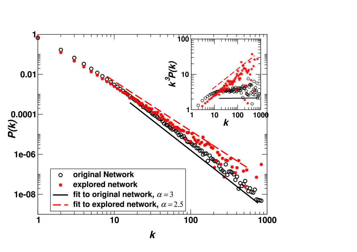
Figure 1: Degree distribution for a Barabási-Albert network grown with $m=1$, with $10^{5}$ nodes. Circles: original network; stars: explored network with $p=0.5$. The best fit to the original network is with $\gamma\simeq 3$, and to the explored network with $\gamma\simeq 2.5$. Inset: rescaled degree distribution $k^{3}P(k)$, such that the data for the original network are constant, and the residual power-law behavior of the explored network is more evident.

The first step in our analysis is to build a BA network, whose degree distribution is shown in Fig.1. Then, starting from a node (we choose a highly connected node) we begin our exploration procedure: 1) each edge connecting that node to its neighbors is followed with probability $p$; edges that are lost at this stage are lost forever 2) from each of the reached nodes, repeat step 1) until no new nodes are reachable. In this procedure, edges to nodes that have already been reached are not followed. The result of this algorithm is a network that has fewer nodes than the original one, and, on the average, fewer links per node, and that is, topologically, a tree. The intuitive result would be that every node sees just a fraction $p$ of its edges, so that all degrees should be reduced of a factor $p$, without consequences on the power-law behavior of $P(k)$. Actually the effects of the probability $p$ are much more dramatic. As it can be seen from our simulations (Fig.1), the measured exponent $\gamma_{m}$ actually changes. For a network grown with $m=1$ and explored with $p=0.5$ the measured exponent is close to $\gamma_{m}=2.5$. We can therefore wonder whether this is a crossover effect, and the correct exponent is recovered for very large networks, or whether this change of exponent is real. A simple analytical argument in favour of this second interpretation can be formulated using the lack of correlations in the BA model. Indeed, since there is no correlation between the degree of a site and the degrees of its neighbors, due to (1) there is no correlation between the age of a node and the age of its neighbors. This allows us to look at exploration during the growth of the network. In particular we can say that, in a growing network formalism, any time a new node is added to the network, we label it as reachable if it connects to at least a reachable site through a followed connection (with probability $p$). We assume that the first site is reachable. Then, the density of reachable nodes at time $t$ is given by

$$\frac{dN(t)}{dt}=1-\left(1-p\int_{0}^{t}\frac{dN(t^{\prime})}{dt^{\prime}}q(t^{\prime})dt^{\prime}\right)^{m}$$ (2)

where $q(t^{\prime})$ is the probability to choose a node introduced in the network between $t^{\prime}$ and $t^{\prime}+dt^{\prime}$: the preferential attachment rule translates to $q(t^{\prime})=1/[2(t\cdot t^{\prime})^{1/2}]$ (this trick is similar to assigning to each node a hidden variable corresponding to the time $t^{\prime}$ at which it entered the network, with a connection probability that depends on the hidden variables of both the new and old nodes; for more details see below BPS03 ; CBS03 ). Since $N(t)$ can grow at most linearly, we make the assumption that $dN(t)/dt\sim t^{\alpha}$ with $\alpha$ expected to be negative. After some algebra, and keeping only the leading terms, we find $\alpha=(mp-1)/2$: as long as $mp<1$ the density of reachable nodes decreases in time. Then, the measured degree distribution can be again obtained from the relation $P_{m}(k)dk=\rho(\tau)d\tau$, with $\rho(\tau)\sim\tau^{\alpha}$, from which we obtain $P_{m}(k)\sim k^{-\gamma_{m}}$, with $\gamma_{m}=2+mp$ For $m=1$, $p=0.5$ we have $\gamma_{m}=2.5$, in agreement with simulations. We expect therefore that, as long as $mp<1$, the measured exponent could be different from the real one.

To check whether the distortion of the exponent is a feature only of BA networks, we have also studied networks generated according to the hidden variables model. Hidden variable networks are characterized by a quantity $x$ (the ”fitness”) assigned to every node and taken from some probability distribution $p(x)$; every pair of nodes $i$ and $j$ is connected then with a probability $q(x_{i},x_{j})$. As a consequence the average degree of a node of fitness $x$ is

$$k(x)=N\int_{U}q(x,x^{\prime})p(x^{\prime})dx^{\prime}$$ (3)

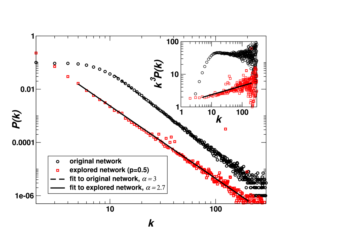
Figure 2: Degree distribution for a hidden variables network with $p(x)\sim x^{-3}$ and $q(x,x^{\prime})\propto x\cdot x^{\prime}$; $10^{5}$ nodes. Circles: original network; squares: explored network with $p=0.5$. The best fit to the original network is with $\gamma\simeq 3$, and to the explored network with $\gamma\simeq 2.7$. Inset: rescaled degree distribution $k^{3}P(k)$, such that the data for the original network are constant, and the residual power-law behavior of the explored network is more evident.

where $N$ is the number of nodes in the network and $U$ is the support of $p(x)$. Eq.3 gives a relation between $k$ and $x$ that can be used in $P(k)dk=p(x)dx$ to obtain $P(k)$. Suitable choices of $p(x)$ and of $q(x,x^{\prime})$ give SF networks. Here we use the same examples provided in CCDM02 , namely Zipf and exponential fitness distributions. Zipf distributed fitnesses are inspired by the idea that many quantities such as personal wealth, company size, city population and others are power-law distributed Zipf . In this case a connection probability $q(x,x^{\prime})\sim x\cdot x^{\prime}$ ensures that the resulting network is SF. Using $p(x)\sim x^{-3}$ we obtain $P(k)\sim k^{-3}$ and in Fig.2 we show that also this network’s exponent has changed following the exploration, with a value $\gamma_{m}\simeq 2.7$.

Next we look at SF networks obtaned using an exponential fitness distribution $p(x)=exp(-x)$ and a connection probability $q(x,x^{\prime})=\theta(x+x^{\prime}-x_{c})$, that is, a link between two nodes of fitness $x$ and $x^{\prime}$ is present only if the sum $x+x^{\prime}>x_{c}$. Eq.3 yelds $k(x)=Ne^{-x_{c}}exp(x)$ and as a consequence $P(k)\sim k^{-2}$ (see Fig.3) CCDM02 . The tree-like exploration of this network shows that, also in this case, the measured exponent can change, $\gamma_{m}\simeq 1.5$. We do not have at the moment an analytical derivation of the measured exponents. Indeed, degree-degree correlations between nearest neighbors and the lack of an explicit time evolution hinder the formulation of some equations similar to (2).

Interestingly, in all cases we have analysed, the measured exponent $\gamma_{m}<\gamma$, an indication that the exploration process penalizes nodes with small degree with respect to nodes with large degree. This is reasonable, since a node with few connections has fewer paths reaching it (and some bottlenecks, since all these paths have ultimately to flow through its few connections) than a high degree node. The final result is therefore that high degree nodes are fairly well represented in the final distribution, whereas the number of nodes with few connections is underestimated. This intuitive picture rationalizes our numerical and analytical finding that the measured exponent is smaller than the real one.

3 Edge-Picking Exploration of Erdös-Rényi and Complete Graphs

The last example is also a good example of how other link detection techniques can change the apparent topological properties of networks in an even more dramatic way, in particular if the probability to detect a link depends on some intrinsic properties of the nodes it connects. Indeed, we can interpret the generation of SF networks from hidden variables as the result of the exploration of complete or Erdös-Rényi ER (ER) networks. Starting from a complete or ER graph, we assign to each node $i$ a variable $x_{i}$ taken from a probability distribution $p(x)=exp(-x)$. Then, we prune the graph by discarding (that is, they are not detected) all those edges that join nodes $i$ and $j$ such that $x_{i}+x_{j}<x_{c}$, with $x_{c}$ a properly chosen threshold. This is tantamount to say that, during the exploration of the graph, the edge between nodes $i$ and $j$ is detected with probability $q(x_{i},x_{j})=\theta(x_{i}+x_{j}-x_{c})$, which brings us back to the formalism used above, that shows that the resulting network is scale-free with degree distribution $P(k)\sim k^{-2}$ (data shown in Fig.3, black symbols, refer to the procedure over a complete graph). Fig.4 (main panel) shows the results for a starting graph that is an Erdös-Rényi network of $12800$ vertices with a connection probability $p=0.025$, corresponding to a graph with average degree $<k>=320$; the threshold $x_{c}=13$. The resulting degrees are power-law distributed with exponent $\gamma\simeq 2$ (black thick line). The peak for large values is what is left of the Poisson distribution of the underlying ER network: whenever a node has a variable $x>x_{c}$, all of its connections are detected, and its degree is not distorted. Since in SF networks a special role is played by hubs, that is, nodes with a very large degree, we checked whether the hubs of the explored network fall into the Poisson cutoff or in the power-law distributed part. The result, shown in the inset of Fig.4 clearly shows that the distribution of the maximum degree nicely obeys a Frechet distribution $P_{max}(k)=(\gamma-1)k^{-\gamma}exp(-k^{-\gamma+1})$ MAA02 , with $\gamma=2.1(1)$. Such a Frechet distribution is indeed the expected distribution of the maxima of set of variables taken from a power-law distribution $k^{-\gamma}$. This implies that, apart from a $1\%$ of the networks (we show the distribution of $k_{max}$ over $10000$ networks), the maximum degree is almost always drawn from the power-law part of the degree distribution, an indication that typical networks can be considered genuinely scale-free.

4 Conclusions

The increase in the amount of real network data is prompting the community to study networks in more detail and to elaborate models able to predict qualitatively, but also quantitatively, the measured properties. Yet, before taking these data by face value, a thorough investigation of the measurement techniques is necessary to ascertain if and what kind of data distortion they could introduce. This is customary in physics, where systematic errors have always to be taken into account and possibly to be corrected, and the same kind of attention should be paid also to data from different disciplines. In this work we have shown, through simple examples, that tree-like explorations, inspired by the traceroute command, can indeed skew the data so that the measured exponent of the degree distribution of a scale-free network can change with respect to the real one. In the simplest case (BA networks), simulations and simple analytical arguments agree with each other. We have also shown that a recently proposed model of SF networks based on hidden variables can be interpreted as an exploration technique leading to the appearence of power-law degree distribution where the underlying network is topologically much simpler.

This work has been supported by the FET Open Project IST-2001-33555 COSIN, and by the OFES-Bern (CH).

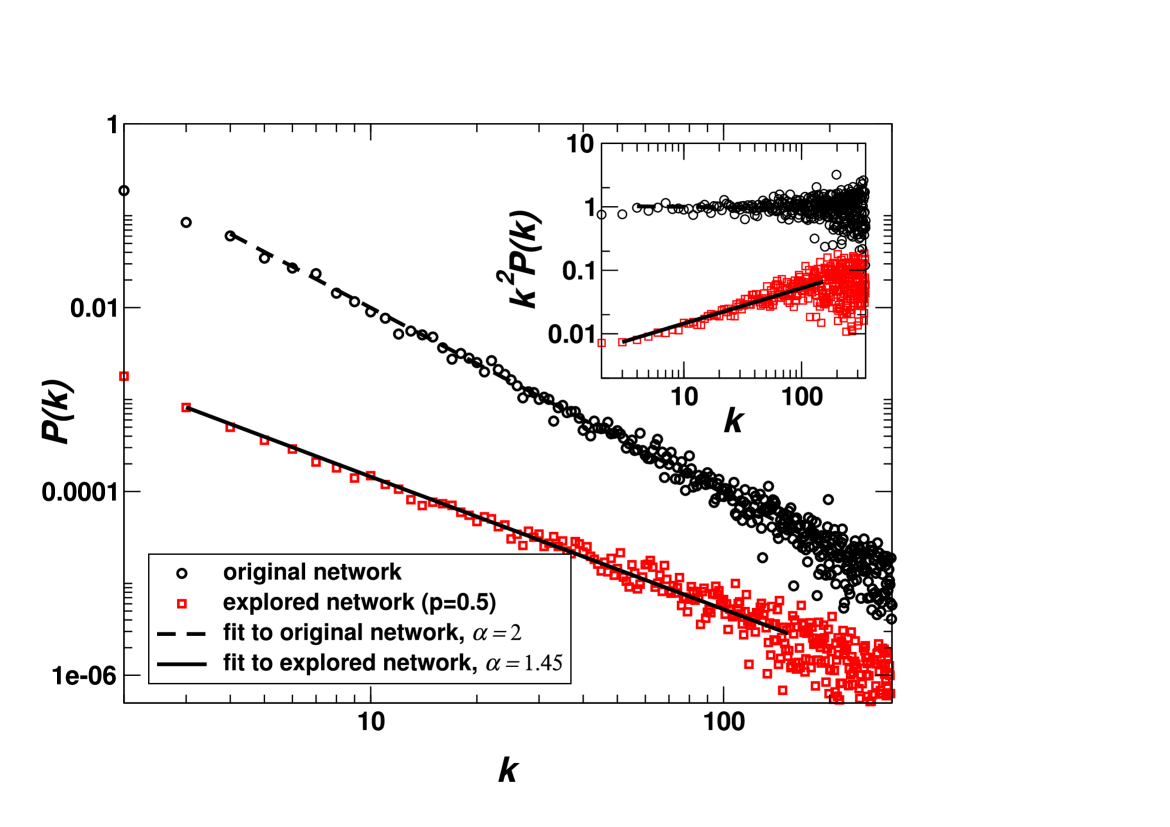
Figure 3: Degree distribution for a hidden variables network with $p(x)\sim e^{-x}$ and $q(x,x^{\prime})=\theta(x+x^{\prime}-x_{c})$; $10^{5}$ nodes. Circles: original network; squares: explored network with $p=0.5$. The best fit to the original network is with $\gamma\simeq 2$, and to the explored network with $\gamma\simeq 1.45$. Inset: rescaled degree distribution $k^{2}P(k)$, such that the data for the original network are constant, and the residual power-law behavior of the explored network is more evident.

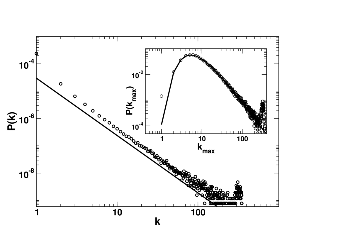
Figure 4: Main panel: Degree distribution for ER networks ($p=0.025$) of $N=12800$ nodes, where every node has been assigned a variable $x$ taken from an exponential distribution. A link between $i$ and $j$ is detected only if $x_{i}+x_{j}>x_{c}=13$; data are averaged over $10000$ realizations. The solid line is $k^{-2}$. Inset: maximum degree distribution for the $10000$ networks; the solid line is a Frechet distribution of exponent $2.1(1)$.

References

- (1) R. Albert and A.L. Barabási, Rev. Mod. Phys. 74, 47 (2002).
- (2) D.J. Watts and S.H. Strogatz, Nature (London) 393, 440 (1998).
- (3) A.L. Barabási and R. Albert, Science 286, 509 (1999).
- (4) G. Caldarelli, R. Marchetti and L. Pietronero, Europhys. Lett. 52, 386 (2000)
- (5) G. Caldarelli, A. Capocci, P. De Los Rios and M.A. Muñoz, Phys. Rev. Lett. 89 , 258702 (2002).
- (6) P.L. Krapivsky, S. Redner and F. Leyvraz, Phys. Rev. Lett. 85, 4629 (2000).
- (7) M. Boguña and R. Pastor-Satorras, Phys. Rev. E 68, 036112 (2003).
- (8) V.D.P. Servedio, G. Caldarelli and P. Buttà, cond-mat/0309659.
- (9) G.K. Zipf, Human Behavior and the Principle of Least Effort, (Addison-Wesley, Cambridge, 1949); M. Marsili and Y.-C. Zhang, Phys. Rev. Lett. 80, 2741 (1998).
- (10) P. Erdös and P. Rényi, Publ. Math. Inst. Hung. Acad. Sci. 5 ,17 (1960).
- (11) A.A. Moreira, J.S. Andrade Jr. and L.A.N. Amaral, Phys. Rev. Lett. 89, 268703 (2002).