Metastable States of the Classical Inertial Infinite-Range-Interaction Heisenberg Ferromagnet: Role of Initial Conditions

Abstract

A system of $N$ classical Heisenberg-like rotators, characterized by infinite-range ferromagnetic interactions, is studied numerically within the microcanonical ensemble through a molecular-dynamics approach. Such a model, known as the classical inertial infinite-range-interaction Heisenberg ferromagnet, exhibits a second-order phase transition within the standard canonical-ensemble solution. The present numerical analysis, which is restricted to an energy density slightly below criticality, compares the effects of different initial conditions for the orientations of the classical rotators. By monitoring the time evolution of the kinetic temperature, we observe that the system may evolve into a metastable state (whose duration increases linearly with $N$), in both cases of maximal and zero initial magnetization, before attaining a second plateau at longer times. Since the kinetic temperatures associated with the second plateau, in the above-mentioned cases, do not coincide, the system may present a three-plateaux (or even more complicated) structure for finite $N$. To our knowledge, this has never before been observed on similar Hamiltonian models, such as the XY version of the present model. It is also shown that the system is sensitive to the way that one breaks the symmetry of the paramagnetic state: different nonzero values for the initial magnetization may lead to sensibly distinct evolutions for the kinetic temperature, whereas different situations with zero initial magnetization all lead to the same structure.

and

1 Introduction

Physical systems characterized by long-range interactions and/or long-range microscopic memories have attracted the attention of many workers recently [1, 2, 3]. The main motivation remains on the fact that such systems present, during longstanding states, inconsistencies with the standard Boltzmann-Gibbs (BG) statistical-mechanics formalism. As an example, the ergodic hypothesis – known to be a pillar of the BG framework – may be violated: a breakdown of ergodicity, leading to a fractal (or even more complex) occupation of phase space, has been observed in some cases [4]. Also, some thermodynamic quantities – expected to increase linearly with the size of the system within the BG framework – like the internal or free energies, may exhibit a nonextensive behavior in these systems. It is becoming evident that a new statistical formalism – more general than the BG framework – should be used to describe such systems properly. Up to now, the most successful proposal appears to be nonextensive statistical mechanics [1, 2, 3], based on a generalization of the BG entropy as proposed in 1988 [5].

Among many interesting systems exhibiting nonextensive behavior, special attention has been dedicated to a classical Hamiltonian system, namely, the inertial long-range-interaction XY model, defined as an assembly of $N$ classical planar rotators interacting through a long-range potential [6, 7, 8, 9, 10, 11, 12, 13, 14, 15, 16, 17]. In the case of infinite-range interactions, i.e., in the limit where the mean-field approach becomes exact for the thermal equilibrium state, a well-known continuous phase transition occurs. If one considers a total energy close to and below the critical energy, there exists a basin of attraction for the initial conditions for which the system gets captured in a metastable state, whose duration increases with $N$, before attaining the terminal thermal equilibrium. Therefore, the particular order that one considers for applying the two relevant limits of this problem, namely, the thermodynamic ($N\rightarrow\infty$) and the long-time ($t\rightarrow\infty$) limits, is extremely pertinent. If one considers the thermodynamic limit before the long-time limit, the system will remain in the metastable state and will never reach the terminal equilibrium state. Moreover, in such a metastable state, the maximum Lyapunov exponent approaches zero (consequently so does the whole Lyapunov-exponent spectrum) [8, 11, 16], indicating that the system is not strongly chaotic. These effects strongly suggest a breakdown of ergodicity, revealing that the phase space will possibly not be equally and completely covered in the infinite-time limit.

As an extension of the above-mentioned system, the inertial classical Heisenberg ferromagnet has been investigated recently [18]. Such a system, which consists of a modification of the well-known Heisenberg model, where the spins are replaced by classical rotators, was considered in the limit of infinite-range interactions. It was studied numerically within the microcanonical ensemble, through a molecular-dynamics approach; the initial conditions used for the spin variables correspond to maximal magnetization, i.e., all rotators aligned along a given direction. Such a system has shown to be even more intriguing than its XY counterpart: the metastable state, observed in the corresponding XY model only near criticality, occurs, in the Heisenberg case, for a whole range of energies, which starts right below criticality and extends up to very high energies [18].

In the present work we investigate the role played by different initial conditions for the spin variables on the dynamical behavior of the inertial classical infinite-range-interaction Heisenberg ferromagnet. It is shown that the dynamical evolution of the kinetic temperature is directly related to the initial magnetization (consistently with what has been recently observed for the XY model [19, 20]). In the next section we define the model and the numerical procedure. In section 3 we present and discuss our results.

2 The Model and Numerical Procedure

The inertial classical infinite-range-interaction Heisenberg ferromagnet is defined through the Hamiltonian

$$H = K+V={1\over 2}\sum_{i=1}^{N}\sum_{\mu}L_{i\mu}^{2}+{1\over 2N}\sum_{i,j=1}^{N}(1-\vec{S}_{i}.\vec{S}_{j})$$ (2.1)

$$= {1\over 2}\sum_{i=1}^{N}\sum_{\mu}L_{i\mu}^{2}+{1\over 2N}\sum_{i,j=1}^{N}\left(1-\sum_{\mu}S_{i\mu}S_{j\mu}\right),$$

where the index $\mu$ ($\mu=x,y,z$) denotes Cartesian components and $L_{i\mu}$ represents the $\mu$-component of the angular momentum (or the rotational velocity, since we are assuming unit inertial moments) of rotator $i$. The rotators are allowed to vary their directions continuously on a sphere of unit radius, leading to the constraint

$$\sum_{\mu}S_{i\mu}^{2}=1\qquad(i=1,2,\cdots N).$$

Due to the close analogy of the above model to the standard classical Heisenberg ferromagnet, we shall, sometimes, refer to the one-dimensional inertial constituents (rotators) as spin variables (see [8] for a discussion about the presence of the factor $1/N$ in front of the potential term).

The BG canonical-ensemble solution of the present model may be worked out easily [18]. The internal energy per particle is given by

$$u={1\over\beta}+{1\over 2}(1-\vec{m}^{2}),$$

where $\beta=1/T$ (herein we work in units of $k_{B}=1)$. In the equation above, $\vec{m}$ represents the magnetization per particle, whose modulus may be calculated by solving the self-consistent equation

$$m\equiv|\vec{m}|={I_{3/2}(\beta m)\over I_{1/2}(\beta m)}={\rm cotanh}(\beta m)-{1\over\beta m},$$

with $I_{k}(y)$ denoting modified Bessel functions of the first kind of order $k$. This model exhibits a well-known continuous phase transition at $T_{c}=1/3$, i.e., $u_{c}=5/6$.

The molecular dynamics follows from a direct integration of the equations of motion

$$\dot{\vec{L}}_{i} = \vec{S}_{i}\times\left({1\over N}\sum_{j=1}^{N}\vec{S}_{j}\right)\qquad(i=1,2,\cdots,N),$$ (2.5a)

$$\dot{\vec{S}}_{i} = \vec{L}_{i}\times\vec{S}_{i}\qquad(i=1,2,\cdots,N),$$ (2.5b)

which correspond to a set of $6N$ equations to be handled numerically. For solving such a set of equations we have used a fourth-order Runge-Kutta-Merson integrator [21] with a time step of 0.05, leading, respectively, to the relative energy and spin-normalization conservations of $10^{-4}$ and $10^{-3}$, or better. The total initial kinetic energy was divided into three equal parts, each of them to be assigned to a given set of Cartesian components of angular velocities $\{L_{i\mu}\}\ (i=1,2,\cdots,N)$. We have always started the system with the so-called water-bag initial conditions [11, 15] for each set of components of angular velocities, i.e., each set $\{L_{i\mu}\}$ was extracted from a symmetric uniform distribution and then, translated and rescaled to have zero total momentum. In what concerns the spin variables, we have started our simulations with a certain configuration, associated with a given magnetization $m(0)$ at time $t=0$. The initial spin configurations employed are described below.

1) Maximal magnetization ($m(0)=m_{z}(0)=1$): all spins aligned along the $z$-axis, which corresponds to zero initial potential energy.

2) Spin directions chosen at random in the upper ($y,z$) semicircle ($z>0$): $m_{x}(0)=m_{y}(0)=0$; $m_{z}(0)=2/\pi$.

3) Spin directions chosen at random in the upper semisphere ($z>0$): $m_{x}(0)=m_{y}(0)=0$; $m_{z}(0)=1/2$.

4) Zero magnetization: $m_{x}(0)=m_{y}(0)=m_{z}(0)=0$. There are several possibilities for such an initial configuration, which differ from one another in the spin-component dispersions. We have used four different choices, listed below.

I) The polar and azimuthal angles, associated with each spin variable, chosen at random, $\theta\in[0,\pi]$, $\phi\in[0,2\pi]$. This corresponds to $\langle S_{x}^{2}\rangle=\langle S_{y}^{2}\rangle=1/4$; $\langle S_{z}^{2}\rangle=1/2$.

II) Spin directions chosen at random in ($x,y$) plane. In this case one has $\langle S_{x}^{2}\rangle=\langle S_{y}^{2}\rangle=1/2$; $\langle S_{z}^{2}\rangle=0$.

III) Spins uniaxially random ($z$ axis): $\langle S_{x}^{2}\rangle=\langle S_{y}^{2}\rangle=0$; $\langle S_{z}^{2}\rangle=1$.

IV) Spherically-symmetric spin distribution: $\langle S_{x}^{2}\rangle=\langle S_{y}^{2}\rangle=\langle S_{z}^{2}\rangle=1/3$.

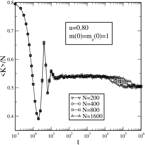
Figure 1: The microcanonical time evolution of $\langle K\rangle/N$ is represented for several system sizes. The initial conditions are water-bag for velocities and maximal magnetization for the spins. For the Hamiltonian defined in Eq. (2.1), energies are dimensionless quantities. The time is also dimensionless and each unit of (physical) time $t$ corresponds to 20 iterations of the equations of motion.

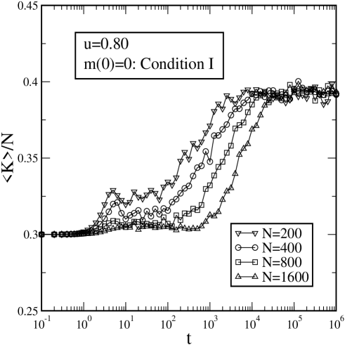
Figure 2: The microcanonical time evolution of $\langle K\rangle/N$ is represented for several system sizes. The initial conditions are water-bag for velocities and zero magnetization (condition I as described in the text) for the spins. For the Hamiltonian defined in Eq. (2.1), energies are dimensionless quantities. The time is also dimensionless and each unit of (physical) time $t$ corresponds to 20 iterations of the equations of motion.

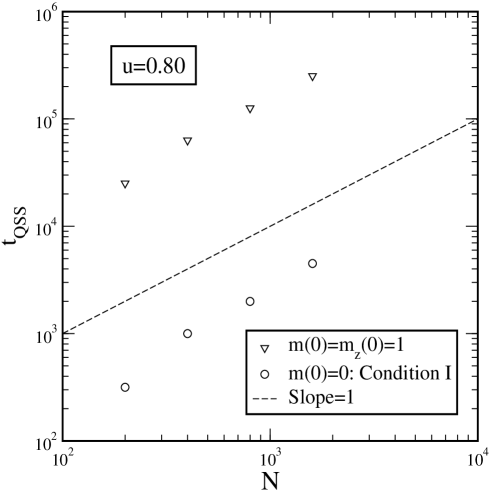
Figure 3: Log-log plots of the lifetime ($t_{\rm QSS}$) of the QSS as a function of $N$, for the two cases considered in Figs. 1 and 2. In both cases, the slope is very close to 1 (represented by the dashed line), in such a way that $t_{\rm QSS}\sim N$.

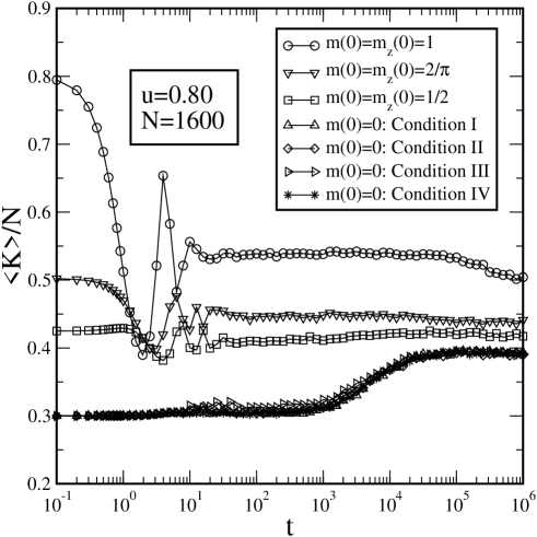
Figure 4: The microcanonical time evolution of $\langle K\rangle/N$ is represented for different initial conditions of the spin variables (see text for a description of such initial conditions). In all cases, the initial conditions for the velocities are water-bag. For the Hamiltonian defined in Eq. (2.1), energies are dimensionless quantities. The time is also dimensionless and each unit of (physical) time $t$ corresponds to 20 iterations of the equations of motion.

3 Results and Discussion

In the results that follow, our measured quantities correspond to averages over $N_{s}$ distinct samples, i.e., different initial sets of $\{L_{i\mu}\}$ and $\{S_{i\mu}\}$. We have considered $N_{s}=20$ ($N=200$), $N_{s}=16$ ($N=400$), $N_{s}=12$ ($N=800$), and $N_{s}=8$ ($N=1600$). Our simulations were carried up to a maximum time $t_{\rm max}=10^{6}$ and each unit of (physical) time corresponds to 20 iterations of the equations of motion. Herein, we restrict our analysis to an internal energy density $u=0.8$, which is slightly below the critical energy ($u_{c}=5/6=0.8333...$). We have investigated, within our microcanonical-ensemble molecular-dynamical approach, how $\langle K\rangle/N$ evolves in time (it should be mentioned that the quantity $\langle K\rangle/N$, which represents an average over different initial conditions of the kinetic energy per particle, when evaluated at the $t\rightarrow\infty$ equilibrium, is expected to be proportional to the temperature).

In Fig. 1 we present the time evolution of $\langle K\rangle/N$, for different values of $N$, in the case of maximal magnetization. One observes that, after a short transient, the system rapidly attains a metastable or quasistationary state (QSS), and only after a long time does the system reach a second state, characterized by a lower value of $\langle K\rangle/N$. A similar effect is observed in the case of zero initial magnetization (condition I as described above), as shown in Fig. 2. However, in the second case, there is no short transient before the QSS, i.e., the system is driven directly to the QSS at the initial time; in addition to that, the second state, obtained at longer times, presents a value of $\langle K\rangle/N$ that is higher than the one of the QSS. In both cases, the lifetime of the QSS ($t_{\rm QSS}$) clearly increases with the size of the system. By defining $t_{\rm QSS}$ as the time at which $\langle K\rangle/N$ presents its halfway between the values at the QSS and the second state, one concludes that such a quantity asymptotically increases, linearly with $N$, i.e., $t_{\rm QSS}\sim N$ for the two cases, as shown in Fig. 3. As a consequence of this, for the cases considered in Figs. 1 and 2, if the thermodynamic limit is performed before the long-time limit, the system will remain in the QSS forever.

In Fig. 4 we compare the time evolution of $\langle K\rangle/N$ for the various initial conditions of the spin variables described above (in all cases, we have considered the size $N=1600$). One observes that this property is not sensitive to the particular way one chooses for setting a zero magnetization at the initial time: all four conditions corresponding to $m(0)=0$ lead to the same time evolution of $\langle K\rangle/N$. However, each one of the three different choices of a nonzero $m(0)$ lead to a distinct time evolution of $\langle K\rangle/N$; this indicates that the time evolution of $\langle K\rangle/N$ is extremely dependent on the particular value chosen for the initial magnetization. Up to the maximal computational time ($t_{\rm max}=10^{6}$) considered in our numerical analysis, we have observed a two-plateaux structure only in the cases $m(0)=1$ and $m(0)=0$ (as shown in Figs. 1–3). However, for the two cases $m(0)=2/\pi$ and $m(0)=1/2$, such an effect is not so clear. An interesting point to stress is that the kinetic temperature is expected to coincide at an infinite time for all cases considered in Fig. 4, i.e., the terminal equilibrium should be independent of the particular initial conditions employed. Therefore, if one considers the $t\rightarrow\infty$ before the thermodynamic limit, there is a possibility of a three-plateaux (or even more complicated) structure for some of the initial conditions considered in Fig. 4.

¿From the results above, one concludes that the inertial infinite-range-interaction Heisenberg ferromagnet is even more intriguing than its XY counterpart. For the latter one has, for energies slightly below the critical energy, a QSS (whose lifetime diverges in the thermodynamic limit) followed by the corresponding terminal equilibrium state; for energies above the critical energy, such a QSS is not present (at least in a clear way). A similar picture to that of the XY model close to criticality occurs in the Heisenberg case for energies considerably higher than the critical energy [18]. Furthermore, close to criticality, the present Heisenberg model shows the possibility of a three-plateaux (or even more complicated) structure, for a fixed system size. The picture that emerges, for explaining such an effect, is that the system may get trapped initially in a small part of phase space; after some time, it will expand to a larger trap (which may, presumably, contain the first one), and so on, until it will finally explore the whole phase space. Obviously, a careful investigation of the properties of such a (possible) second QSS requires a high computational effort. However, if one considers the order of the two relevant limits of this problem in such a way as to perform the thermodynamic limit before the long-time limit, the system will remain in the first QSS forever; all further states – including other possible QSS’s, as well as the terminal equilibrium state – will not be accessible to the system. In this case, the only relevant state is the first QSS, which in the present Heisenberg model, may depend on the particular initial conditions employed.

References

- [1] Nonextensive Statistical Mechanics and Its Applications, edited by S. Abe and Y. Okamoto, Lecture Notes in Physics (Springer-Verlag, Heidelberg, 2001).
- [2] Classical and Quantum Complexity and Nonextensive Thermodynamics, Chaos Solitons and Fractals 13 (2002), edited by P. Grigolini, C. Tsallis, and B. J. West.
- [3] Nonextensive Entropy – Interdisciplinary Applications, edited by M. Gell-Mann and C. Tsallis (Oxford University Press, Oxford, 2004) in press.
- [4] F. Baldovin, E. Brigatti, and C. Tsallis, Phys. Lett. A 320, 254 (2004).
- [5] C. Tsallis, J. Stat. Phys. 52, 479 (1988).
- [6] M. Antoni and S. Ruffo, Phys. Rev. E 52, 2361 (1995).
- [7] V. Latora, A. Rapisarda, and S. Ruffo, Phys. Rev. Lett. 80, 692 (1998).
- [8] C. Anteneodo and C. Tsallis, Phys. Rev. Lett. 80, 5313 (1998).
- [9] V. Latora, A. Rapisarda, and S. Ruffo, Phys. Rev. Lett. 83, 2104 (1999).
- [10] V. Latora, A. Rapisarda, and S. Ruffo, Physica A 280, 81 (2000).
- [11] V. Latora, A. Rapisarda, and C. Tsallis, Phys. Rev. E 64, 056134 (2001).
- [12] M. A. Montemurro, F. A. Tamarit and C. Anteneodo, Phys. Rev. E 67, 031106 (2003).
- [13] A. Campa, A. Giansanti, and D. Moroni, Phys. Rev. E 62, 303 (2000).
- [14] A. Campa, A. Giansanti, D. Moroni, and C. Tsallis, Phys. Lett. A 286, 251 (2001).
- [15] V. Latora, A. Rapisarda, and C. Tsallis, Physica A 305, 129 (2002).
- [16] B. J. C. Cabral and C. Tsallis, Phys. Rev. E 66, 065101(R) (2002).
- [17] Y. Y. Yamaguchi, J. Barré, F. Bouchet, T. Dauxois, and S. Ruffo, cond-mat/0312480.
- [18] F. D. Nobre and C. Tsallis, Phys. Rev. E 68, 036115 (2003).
- [19] A. Pluchino, V. Latora, and A. Rapisarda, cond-mat/0303081.
- [20] A. Pluchino, V. Latora, and A. Rapisarda, cond-mat/0312425.
- [21] L. Lapidus and J.H. Seinfeld, Numerical Solution of Ordinary Differential Equations (Academic Press, London, 1971).