Topological percolation on a square lattice

Abstract

We investigate the formation of an infinite cluster of entangled threads in a (2+1)–dimensional system. We demonstrate that topological percolation belongs to the universality class of the standard 2D bond percolation. We compute the topological percolation threshold and the critical exponents of topological phase transition. Our numerical check confirms well obtained analytical results.

I Introduction

In this paper we would like to link together two different subjects, percolation and topology, which since now were considered separately in physical literature. The problem discussed below deals with entanglement of threads: we apply to the threads a random set of operators of ”windings” and check whether two initial sets of threads become mutually entangled. The transition between entangled and nonentangled states may be considered as a ”topological phase transition”. We investigate the critical properties of such transition and show that it can be mapped onto the percolation problem. We also numerically investigate the critical exponent of the topological percolation and demonstrate that it is equal to the one of the two dimensional percolation.

Let us remind the general formulation of the bond percolation problem. Consider a planar (for example, square) lattice of size $L\times L$ ($L\to\infty$) with elementary cell of size $1\times 1$. Each bond on the lattice is occupied with the probability $p$ independently on all other bonds (i.e. with the probability $1-p$ the bond is left empty). There exists a critical value $p=p_{c}$ at which the infinitely large connected cluster of occupied bonds is formed. In other words, above $p_{c}$ at least two bonds belonging to opposite sides of the lattice are connected by a path of occupied bonds. It is known that for the two dimensional bond percolation $p_{c}=\frac{1}{2}$ SA . The 2D percolation has been extensively studied during last decade. The scaling behavior of crossing probability (the probability to percolate in, say, horizontal direction as a function of $p$) in the vicinity of $p_{c}$ is defined by the correlation length exponent HL1 ; HL2 ; HL3 . A deep insight of scaling at the critical point has been achieved using the conformal approaches Lang1 ; Lang2 ; Lang3 ; Cardy0 ; Cardy1 ; Watts .

The problem discussed below deals with entanglement of threads of finite length growing from a two-dimensional substrate. Apparently for the first time the continuous version of the same problem has been treated in Alava1 . Let us specify the model under consideration. Consider the two-dimensional square lattice of size $L\times L$, serving as the ”substrate” from which the threads start to grow. Each time moment one pair of nearest neighboring (along $x$– or $y$–axes) lines on the lattice may produce the full-turn entanglement. We assign the ”generators” $g_{x},\,g_{x}^{-1}$ to the full clockwise and counterclockwise turns along $x$–axis, and $g_{y},\,g_{y}^{-1}$ to the full clockwise and counterclockwise turns along $y$–axis, and as it is schematically shown in the figure 1.

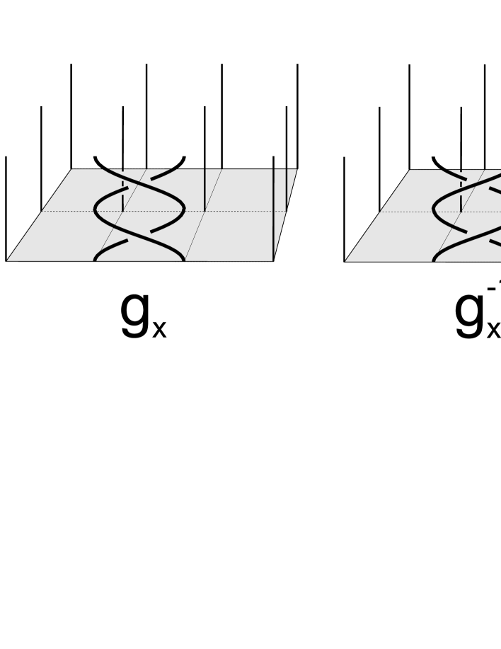
Figure 1: Generators of elementary entanglements of neighboring threads.

Let us choose randomly any pair of nearest neighboring threads on the lattice and entangle them with the probability $q$; with the probability $1-q$ we leave the pair of threads unentangled. If we decide to entangle the threads, then we do that clockwise with the probability $r^{+}$ and counterclockwise with the probability $r^{-}=1-r^{+}$. Later on we shall consider only two extremal cases: i) $r^{+}=1$, meaning that all neighboring threads are entangled clockwise overall the lattice, and ii) $r^{+}=\frac{1}{2}$, denoting the situation when each entanglement may be either clockwise or counterclockwise with equal probabilities. Let us stress that for any $r^{\pm}\neq 1$ there is the possibility to unwind the neighboring threads, what essentially complicates the problem. The general structure of the bunch of entangled directed threads is shown in the Fig.2.

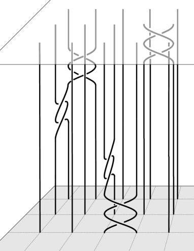
Figure 2: Bunch of entangled threads.

Now we are in position to formulate the main question of our interest. Suppose that each time step we apply randomly one clockwise or counterclockwise winding to the top ends of randomly chosen pair of neighboring threads on the lattice of size $L\times L$. When time passes, more and more threads become topologically connected (entangled). We would like to compute the typical (critical) number of applied windings at which the threads on the opposite sides of the substrate form the topologically connected cluster, i.e. become entangled. This model sets the concept of ”topological percolation”.

II Entanglements and the locally free group

The generators $g_{x},\,g_{x}^{-1},\,g_{y},\,g_{y}^{-1}$ of full turns are defined for each pair of nearest neighboring threads and, hence, should depend on the lattice coordinate (in Fig.1 the corresponding lattice indices are omitted for simplicity): $g_{x}(i,j)$ – a clockwise ($+$)–generator and $g^{-1}_{x}(i,j)$ – a counterclockwise ($-$)–generator of threads $(i,j)$ and $(i+1,j)$ along $x$–axis; $g_{y}(i,j)$ – a clockwise ($+$)–generator and $g^{-1}_{y}(i,j)$ – a counterclockwise ($-$)–generator of threads $(i,j)$ and $(i+1,j)$ along $y$–axis. The pair of indices $(i,j)$ is attributed to the $(x,y)$ coordinates of a left or a bottom threads in a pair; $i$ and $j$ run along $x$ and $y$ axes correspondingly.

The whole set of generators $\{g_{x}(i,j),\,g_{x}^{-1}(i,j),\,g_{y}(i,j),\,g_{y}^{-1}(i,j)\}$ (for all $1\leq\{i,j\}\leq N-1$) sets the surface locally free group ${\cal LF}_{2D}$ paris ; ne_bi . It is known ve_ne_bi that each generator $g$ can be represented in a form $g=\sigma^{2}$ (we have omitted indices for brevity), where $\sigma$ is the braid group generator. The generators $g$ obey the following commutation relations:

$$\left\{\begin{array}[]{llll}g^{s}_{x}(i,j)g^{s}_{x}(i^{\prime},j^{\prime})&=&g^{s}_{x}(i^{\prime},j^{\prime})g^{s}_{x}(i,j)&\mbox{if $|i-i^{\prime}|>1$ or $|j-j^{\prime}|>0$}\vskip 6.0pt plus 2.0pt minus 2.0pt\\ g^{s}_{y}(i,j)g^{s}_{y}(i^{\prime},j^{\prime})&=&g^{s}_{y}(i^{\prime},j^{\prime})g^{s}_{y}(i,j)&\mbox{if $|i-i^{\prime}|>0$ or $|j-j^{\prime}|>1$}\vskip 6.0pt plus 2.0pt minus 2.0pt\\ g^{s}_{x}(i,j)g^{\pm s}_{y}(i^{\prime},j^{\prime})&=&g^{\pm s}_{y}(i^{\prime},j^{\prime})g_{x}(i,j)&\mbox{if $i-i^{\prime}\neq 0,1$ or $j^{\prime}-j\neq 0,1$}\vskip 6.0pt plus 2.0pt minus 2.0pt\\ g^{s}_{x}(i,j)g^{-s}_{x}(i,j)&=&g^{s}_{y}(i,j)g^{-s}_{y}(i,j)=1&\end{array}\right.$$ (1)

where we have attributed $s="+"$ for $g$ and $s="-"$ for $g^{-1}$.

We can reformulate our geometrical problem of entanglement of threads in terms of random walk on the group ${\cal LF}_{2D}$. Consider the square lattice of size $L\times L$. There are $N=2L^{2}$ threads passing through the vertices of the lattice along $z$–direction normal to the plane $(xy)$. Here and later we assume the square geometry, but we can consider any other lattices in the same way. We generate the random word in terms of ”letters”–generators of the group ${\cal LF}_{2D}$. Namely, we randomly apply one after another generators of ${\cal LF}_{2D}$ (with appropriate probabilities) to the open ends of threads, respecting the commutation relations (1). Let us repeat that the generators acting along $x$– and $y$–axes have equal probabilities. The ($+$) and ($-$)–generators have correspondingly the probabilities $r^{+}$ and $r^{-}=1-r^{+}$.

When a random sequence of $M$ ”letters” is generated, we check whether there are at least two threads on opposite sides of the lattice which are topologically connected to each other (i.e. whether they belong to the same cluster of entangled lines). We are interested in statistics of such cross–lattice entanglements averaged over different realizations of random sequences of ”letters”. As one sees later, this problem has straightforward relation to the two-dimensional bond percolation on the same lattice.

III Geometry of entanglements and bond percolation

Let us describe a simple geometric model which visualizes the commutation relations (1) of the surface locally free group, making them very transparent. We associate the ”white” cells to the generators $g_{x}(i,j)$ and $g_{y}(i,j)$ and ”black” cells to the inverse generators $g_{x}^{-1}(i,j)$ and $g_{y}^{-1}(i,j)$. We drop cells randomly, one cell per each time step. The commutation relations (1) specify the geometry of the heap constituted by falling cells. For example, if the falling cell and one of the previous cells have only one common edge, the upper cell remains on the lower one; if however the cell falls strictly on the cell with opposite color, these two cells annihilate. The figure (3) shows the particular example of two pairs of non-commuting (left) and commuting (right) generators.

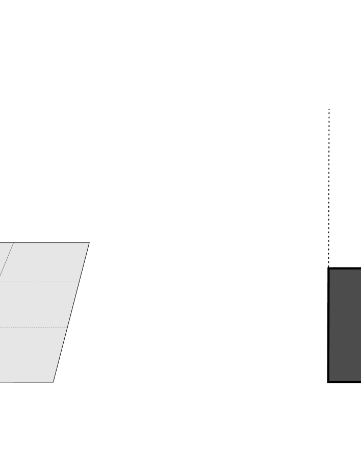
Figure 3: Visualization of some commutation relations in the group ${\cal LF}_{2D}$.

The general view of growing heap of white–black cells is shown in Fig.4. This picture demonstrates the typical configuration of cells for the system size $L=10$ and $r^{+}=0.5$.

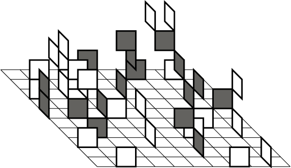
Figure 4: Typical heap of colored cells representing clusters of entangled threads.

Remind that any white (black) cell corresponds to the full clockwise (counterclockwise) turn of neighboring vertical threads. The empty horizontal intervals between cells mean that the threads in these intervals are not entangled.

Consider now the projection of the heap of cells onto the horizontal $xy$–plane (the base surface). In this projection the single thread is represented by a dot (a lattice site). Each falling cell corresponds to the bond between two neighboring sites. If at least one cell in a projection (independent on the cell color) covers some bond, we close this bond. Otherwise we leave this bond open.

It is not difficult to establish the bijection between entanglements and the standard percolation. Two distant threads are linked together (entangled) by some sequence of full turns of nearest neighboring threads if and only if the lattice sites corresponding to these threads belong to the same connected cluster of closed bonds. Otherwise these distant threads are not entangled. Thus, if a cluster of connected sites touches the opposite sides of the lattice, then we can always find two threads on opposite sites of the lattice entangled to each other.

There are two formulations of the classical theory of bond percolation: canonical and grand canonical. In the canonical approach the averaging is performed over configurations with preserved number of closed bonds $S$ on the lattice and, hence, the normalized concentration of closed bonds $s=\frac{S}{N}$ is also fixed. In the grand canonical approach only the probability $p$ of a bond to be closed is fixed, while the concentration $s$ fluctuates near the average value $\left<s\right>=p$. These two formulations are linked together in a simple way. If we know, for example, the crossing probability in the horizontal direction, $\pi_{h}(S)$, for the canonical distribution, we can obtain the same quantity in the grand canonical formalism by averaging $\pi_{h}(S)$ over the Binomial distribution

$$\pi_{h}(p,L)=\sum\limits_{S=0}^{N}P_{b}(S;p,N)\pi_{h}(S,L)$$ (2)

where $P_{b}(S;p,N)$ is the probability to have exactly $S$ closed bonds on the lattice of size $L$ with $N=2L^{2}$ bonds for fixed value of the bond closure probability $p$:

$$P_{b}(S;p,N)=\frac{N!}{S!(N-S)!}\,p^{S}(1-p)^{N-S}$$ (3)

Here and below we assume that a function of the argument $S$ (or of $s$) corresponds to the canonical distribution, while a function of the argument $p$ corresponds to the grand canonical distribution. The capital letters $S$ and $M$ denote the number of closed bonds and number of dropped cells for the entire lattice, while the letters $s=\frac{S}{N}$ and $m=\frac{M}{N}$ denote the same quantities normalized per number of bonds.

In Refs. NZ1 ; NZ2 ; NZ3 the relation (2) has been used for very efficient numerical simulation of the grand canonical crossing probability by using the canonical one, which is more fast and simple in practical applications.

Let us note that eq.(2) sets the general relation between two different ensembles (grand canonical and canonical) and we shall exploit this relation for our goals to establish connection between the standard grand canonical formulation of crossing probability and our canonical formulation of percolation produced by growing heap. Namely, in our model for each lattice size $L$ and specified value $r^{+}$ we randomly add each time moment the new cell to the heap and stop at the time moment when $M$ cells are added. After that we check the horizontal spanning property of obtained configuration of closed bonds by using the Hoshen-Kopelman algorithm HK . Then we perform averaging over $10^{4}$ different configurations and obtain the topological crossing probability $\pi_{t}(M;r^{+},L)$. The only difference from the usual crossing probability $\pi_{h}(p,L)$ is that we generate each configuration of closed bonds by adding cells to the heap instead of closing each bond independently. The crucial difference appears for $r^{+}\neq 0;\,1$, i.e. when annihilation is allowed. Let us remind that for topological percolation each closed bond is the projection of one (or several) cells from the heap to the base surface.

Figure 5: The topological crossing probability $\pi_{t}(m;r^{+},L)$ as a function of $m=M/N$ for $r^{+}=1;\,0.5$ and crossing probability $\pi_{h}(s;L)$ of bond percolation, canonical case.

In the Fig.5 we have plotted the topological crossing probability $\pi_{t}(m;r^{+},L)$ as a function of $m=\frac{M}{N}$ for two cases $r^{+}=1;\,0.5$. In the same figure the crossing probability $\pi_{h}(s;L)$ of the standard bond percolation is plotted for comparison as a function of $s$. The graph for the usual percolation $\pi_{h}(s;L)$ crosses the horizontal line $0.5$ at the critical point $s_{\rm c}=\frac{1}{2}$. The slop of $\pi_{h}(s;L)$ is maximal at the critical point. The same construction can be used for the topological crossing probability. The graph $\pi_{t}(m;r^{+},L)$ for $r=1$ crosses the horizontal line $s_{\rm c}\frac{1}{2}$ at the point with the maximal slop, and the graphs for different lattice sizes $L$ cross each other at that point. As we see later, this is the critical point of topological percolation for $r^{+}=1$. The the similar behavior (however with different critical point) is valid for $r=0.5$.

We can express the topological probability $\pi_{t}(M;r^{+}=1,L)$ via the crossing probability $\pi_{h}(M;L)$ in the way similar to eq. (2). Thus our next goal is to find the probability distribution $P_{t}(S;M,N)$ of having $S$ closed bonds on the $N$–bond lattice if we have added $M$ cells to a heap. This probability distribution $P_{t}(S;M,N)$ plays the same role for the topological percolation as the binomial distribution $P_{b}(S;p,N)$ plays the role for the percolation in the ”canonical” consideration. To begin with, let us consider only clockwise local turns ($r^{+}=1$) because in this case there are no cancellations of opposite turns, and the problem becomes essentially more simple. We denote this case ”the irreversible topological percolation”.

Consider some particular configuration on the lattice with $S$ closed bonds and apply the mean–field consideration. Adding one extra cell to a heap, we see that with probability $s=\frac{S}{N}$ this cell hits closed already bond and does not change the number of closed bonds. However with probability $1-s$ the new cell hits the open bond and closes it increasing the number of closed bonds by one. Therefore, we can write down the master equation for $P_{t}(S;M,N)$ on the lattice $L$:

$$P_{t}(S+1;M+1,N)=\frac{S+1}{N}P_{t}(S+1;M,N)+\left(1-\frac{S}{N}\right)P_{t}(S;M,N)$$ (4)

with the following initial and boundary conditions:

$$\left\{\begin{array}[]{l}P_{t}(S=0;M=0,N)=1\\ P_{t}(S=0;M\geq 1,N)=0\\ P_{t}(S=1;M=1,N)=1\\ P_{t}(S=1;M\neq 1,N)=0\end{array}\right.$$ (5)

It is easy to solve this problem by the method of generating functions. Define

$$Q(t,z)=\sum_{M=0}^{\infty}\sum_{S=0}^{\infty}P(S;M,N)t^{S}z^{M}$$ (6)

Eqs. (4)–(5) in terms of $Q(t,z)$ read

$$\frac{1}{N}\frac{\partial Q(t,z)}{\partial t}=\frac{1-tz}{tz(1-t)}Q(t,z)-\frac{1}{tz(1-t)}$$ (7)

The solution of (7) (properly normalized) is as follows

$$Q(t,z)=(1-t)^{\frac{N(1-z)}{z}}\,{{}_{2}F_{1}}\left(-\frac{N}{z},1+N-\frac{N}{z},1-\frac{N}{z},t\right)$$ (8)

where ${{}_{2}F_{1}}(...)$ is the standard hypergeometric function—see, for example abramowitz .

Now we can straightforwardly compute the mathematical expectation $\left<S(M,N)\right>$ and the dispersion $\left<\Delta S^{2}(M,N)\right>=\left<S^{2}(M,N)\right>-\left<S(M,N)\right>^{2}$:

$$\begin{array}[]{rll}\left<S(M,N)\right>&=&\displaystyle\frac{1}{2\pi i}\oint_{C}\frac{dz}{z^{M+1}}\left[\frac{dQ(t,z)}{dt}\bigg{|}_{t=1}\right]=N\left\{1-\left(\frac{N-1}{N}\right)^{M}\right\}\vskip 6.0pt plus 2.0pt minus 2.0pt\\ \left<S(M,N)(S(M,N)-1)\right>&=&\displaystyle\frac{1}{2\pi i}\oint_{C}\frac{dz}{z^{M+1}}\left[\frac{d^{2}Q(t,z)}{dt^{2}}\bigg{|}_{t=1}\right]\vskip 6.0pt plus 2.0pt minus 2.0pt\\ &=&\displaystyle N(N-1)\left\{1-2\left(\frac{N-1}{N}\right)^{M}+\left(\frac{N-2}{N}\right)^{M}\right\}\end{array}$$ (9)

where the contour $C$ surrounds the point $z=0$. Therefore

$$\begin{array}[]{lll}\left<\Delta S^{2}(M,N)\right>&=&\left<S(M,N)(S(M,N)-1)\right>+\left<S(M,N)\right>-\left<S(M,N)\right>^{2}\vskip 6.0pt plus 2.0pt minus 2.0pt\\ &=&\displaystyle N(N-1)\left(\frac{N-2}{N}\right)^{M}-N^{2}\left(\frac{N-1}{N}\right)^{2M}+N\left(\frac{N-1}{N}\right)^{M}\end{array}$$ (10)

Let us evaluate the normalized expectation $\left<s(m,L)\right>=\frac{\left<S(M,N)\right>}{N}$ and the dispersion $\left<\Delta s^{2}(m,L)\right>=\frac{\left<\Delta S^{2}(M,N)\right>}{N^{2}}$, where $N=2L^{2},\;m=\frac{M}{N}$. In the asymptotic regime, where $N\gg 1,\,M\gg 1$ and $m=\frac{M}{N}={\rm const}$, we can rewrite (9) for normalized quantities in the limit $L\to\infty$ as follows

$$\left<s(m,N)\right>\equiv\frac{\left<S\right>}{N}=1-\lim_{N\to\infty}\left[\left(1-\frac{1}{N}\right)^{N}\right]^{m}=1-e^{-m}$$ (11)

and

$$\frac{\left<S^{2}\right>}{N}=\lim_{N\to\infty}\left[(N-1)\left(1-\frac{2}{N}\right)^{Nm}-N\left(1-\frac{1}{N}\right)^{2Nm}+\left(1-\frac{1}{N}\right)^{Nm}\right]=e^{-m}-(1+m)e^{-2m}$$ (12)

On the basis of (12) we expect for all $r^{+}$

$$\left<\Delta s^{2}(m;r^{+},L)\right><\frac{\rm const}{N}=\frac{\rm const}{2L^{2}}$$ (13)

Now we are in position to attack the ”reversible topological percolation”, i.e. the case $r^{+}=0.5$ when both clockwise and counterclockwise turns are allowed. First of all we estimate the maximal number of annihilated cells. In ne_bi the average number $\left<H\right>$ of the most top cells (called ”the roof”) of the heap in the stationary regime $M\gg N$ has been analytically computed. Only those cells are accessible for cancellations. We reproduce here the result of ne_bi :

$$\left<h(m,N)\right>=\frac{\left<H(M,N)\right>}{N}=\frac{1}{7}$$ (14)

For convenience we have reproduced in Appendix the derivation of this expression.

Following the methods developed in the works ne_bi ; ne_des ; des one can also compute the dependence $\left<h(M,N)\right>$ in the intermediate regime $M<N$. The function $\left<h(m,N)\right>$ in all regimes is well approximated by the curve

$$\left<h(m,N)\right>=\frac{1}{7}(1-e^{-7m})$$ (15)

The analytic derivation of this expression is presented in Appendix. To verify (15) we compare in Fig.6 the data of numerical simulations for the average size of the roof $\left<h(m;r^{+},L)\right>$ for $r^{+}=0.5$, $L=128$ with eq.(15). One sees that the function $\left<h(M,N)\right>=\frac{1}{7}(1-e^{-7m})$ perfectly fits the data.

Figure 6: Dependence the size of the roof of the heap $h(m;r^{+},L)$ for $r^{+}=0.5$ and $L=128$ in comparison with $\frac{1}{7}(1-e^{-7m})$.

Let us make one step back and demonstrate that for $r^{+}=1$ we can arrive at eq. (11) in a simple way. Suppose that some configuration of cells covers the base surface. If we put one more cell, it hits the empty bond and increases the number of closed bonds by one with the probability $1-s$, while it hits the closed bond and does not change the number of closed bonds with the probability $s$. These conditions are summarized in the table below:

$$\Delta s(m,r^{+}=1)=\left\{\begin{array}[]{rl}+1&\mbox{with the probability $1-s$}\vskip 6.0pt plus 2.0pt minus 2.0pt\\ 0&\mbox{with the probability $s$}\end{array}\right.$$ (16)

So, we have

$$\left\{\begin{array}[]{l}\displaystyle\frac{d\left<s(m,r=1)\right>}{dm}=1-s(m)\vskip 6.0pt plus 2.0pt minus 2.0pt\\ s(m=0)=0\end{array}\right.$$ (17)

The solution to this equation is (11).

We modify now eq. (17) to catch the ”reversible topological percolation” ($r^{+}=0.5$), taking into account the annihilation. We have stressed that the annihilation of cells occurs in the roof only. Each bond of the roof is either black or white with the probability $\frac{1}{2}$. Hence the total probability of annihilation is about $\frac{1}{2}\left<h(m;r^{+},L)\right>$. Moreover, the bond in the base surface becomes ”open” if and only if the cell of the roof is single in the corresponding column, i.e. below the given roof’s cell there are no other cells in the same column. The probability to have empty set of $1-\left<s(m)\right>$ columns is given by the solution of eq.(17): $1-\left<s(m)\right>=e^{-m}$. Hence, the probability $p_{\rm cond}$ of annihilation of the roof’s cell under the condition that below this roof’s cell there are no other cells in the same column (assuming the uniform distribution of the roof’s cells and empty columns), is given by the product:

$$p_{\rm cond}=\frac{1}{2}\left<h(m;r^{+}=0.5)\right>\times e^{-m}=\frac{e^{-m}}{14}(1-e^{-7m})$$ (18)

Therefore

$$\Delta s(m,r^{+}=0.5)=\left\{\begin{array}[]{rl}-1&\mbox{with the probability $\frac{e^{-m}}{14}(1-e^{-7m})$}\vskip 6.0pt plus 2.0pt minus 2.0pt\\ 0&\mbox{with the probability $s-\frac{e^{-m}}{14}(1-e^{-7m})$}\vskip 6.0pt plus 2.0pt minus 2.0pt\\ +1&\mbox{with the probability $1-s$}\end{array}\right.$$ (19)

Hence, we can write

$$\left\{\begin{array}[]{l}\displaystyle\frac{d\left<s(m),r^{+}=0.5\right>}{dm}=1-s(m)-\frac{e^{-m}}{14}\left(1-e^{-7m}\right)\vskip 6.0pt plus 2.0pt minus 2.0pt\\ s(m=0)=0\end{array}\right.$$ (20)

The solution to eq. (20) reads

$$\left<s(m;r^{+}=0.5)\right>=1-\frac{e^{-8m}}{98}-\frac{97\,e^{-m}}{98}-\frac{m\,e^{-m}}{14}$$ (21)

Figure 7: Comparison of $\left<s(m;r^{+},L)\right>$ for $r=1,0.5$ and $L=128$ with the approximation functions.

In Fig.7 we plot the numerical data for $\left<s(m;r^{+},L)\right>$ for $r^{+}=1,0.5$ and $L=128$ (crosses). We see, that data for $r^{+}=1$ is in the excellent agreement with eq. (11). For comparison, in the same figure we plot also the analytic expression (21) for the ”reversible topological percolation”. As one sees, this curve fits rather well the corresponding numerical simulations.

Let us introduce the probability distribution for normalized quantities $P_{t}(m,s,L)=2L^{2}\,P_{t}(2L^{2}s,2L^{2}m,2L^{2})$. We can write (at least for the critical region) the scaling expression for the crossing probability

$$\pi_{h}(s,L)\simeq f\left((s-s_{c})L^{1/\nu}\right)$$ (22)

where $\nu=\frac{4}{3}$ is the critical exponent of the correlation length for the percolation. Therefore

$$\left.\frac{\partial^{2}\pi_{h}(s,L)}{\partial s^{2}}\right|_{s\to s_{c}}\simeq L^{2/\nu}\,f^{\prime\prime}((s-s_{c})L^{1/\nu})$$ (23)

For $S\gg 1$, $N\gg 1$ we have

$$\begin{array}[]{lll}\pi_{t}(m_{c},L)&=&\displaystyle\sum_{S=0}^{N}P_{t}(S;M_{c},N)\pi_{h}(S/(2L^{2}),L)\simeq\int_{0}^{1}P_{t}(s;m_{c},L)\pi_{h}(s,L)ds\vskip 6.0pt plus 2.0pt minus 2.0pt\\ &\simeq&\displaystyle\int_{0}^{1}P_{t}(s;m_{c},L)\left(\pi_{h}(s_{c},L)+\left.\frac{\partial\pi_{h}(s,L)}{\partial s}\right|_{s=s_{c}}\Delta s+\left.\frac{\partial^{2}\pi_{h}(s,L)}{\partial s^{2}}\right|_{s=s_{c}}\Delta s^{2}+o(\Delta s^{2})\right)ds\vskip 6.0pt plus 2.0pt minus 2.0pt\\ &\simeq&\displaystyle\pi_{h}(s_{c},L)+\left.\frac{\partial^{2}\pi_{h}(s,L)}{\partial s^{2}}\right|_{s=s_{c}}\left<\Delta s^{2}(m,L)\right>\simeq\pi_{h}(s,L)+L^{2/\nu-2}f^{\prime\prime}(s-s_{c}))+o(L^{2/\nu-2})\end{array}$$ (24)

where $\Delta s=s-s_{c}$, $s_{c}=1-e^{-m_{c}}$ and the function $f(s-s_{c})$ is regular in the vicinity of the point $s_{c}$. We use the condition (13) for the dispersion $\left<\Delta s^{2}(m,L)\right>$. Hence for large lattices one has

$$\lim_{L\to\infty}\pi_{t}(m;\,r=1,\,L)=\pi_{h}\Big{(}1-e^{-m},\,L\Big{)}$$ (25)

The bond percolation on infinite square lattice occurs at the concentration of bonds $s_{c}=p_{c}=\frac{1}{2}$. Hence, using (11), we get the critical concentration of local turns (or falling cells) $m_{\rm c}=\frac{M_{\rm c}}{N}$ at the percolation threshold in the limit $L\gg 1$ for irreversible (($r^{+}=1$) and reversible ($r^{+}=0.5$) cases:

$$\left\{\begin{array}[]{ll}\displaystyle m_{\rm c}(r^{+}=1)=\ln 2\simeq 0.693&\quad\mbox{for $r^{+}=1$}\vskip 6.0pt plus 2.0pt minus 2.0pt\\ \displaystyle m_{\rm c}(r^{+}=0.5)\approx 0.734&\quad\mbox{for $r^{+}=0.5$}\end{array}\right.$$ (26)

These solutions are obtained from eqs. (11) and (21) correspondingly:

$$\left\{\begin{array}[]{l}s_{\rm c}=\frac{1}{2}=1-e^{-m_{\rm c}}\vskip 6.0pt plus 2.0pt minus 2.0pt\\ s_{\rm c}=\frac{1}{2}=1-\frac{e^{-8m_{\rm c}}}{98}-\frac{97\,e^{-m_{\rm c}}}{98}-\frac{m\,e^{-m_{\rm c}}}{14}\end{array}\right.$$

The values (26) are in good agreement with the data of numerical simulations shown in Fig.5.

Figure 8: The topological crossing probability $\pi_{t}(s;r^{+},L)$ as a function of the average number of the closed bonds $s=1-\exp(-m)$ for $r=0.5,1$ and crossing probability $\pi_{h}(s;L)$ of bond percolation, canonical case.

In the Fig.8 we show by symbols the topological crossing probability $\pi_{t}$ as a function of a variable $s=1-\exp(-m)$ for $r^{+}=1,0.5$ and $L=32,64,128$. In the same figure we plot the crossing probability of bond percolation $\pi_{h}(s;L)$ for the canonical case by lines. One sees that the symbols for $r^{+}=1$ lie on the appropriate lines. Our investigation allows us to conclude that the topological percolation belongs to the universality class of the two dimensional percolation. We confirm this statement numerically. Namely, we extract the correlation length exponent $\nu=4/3$ from the numerical data shown in the Fig.8. The outline of our construction is as follows. The eq.(22) allows us to conclude that the derivative of the crossing probability at the critical point scales with the lattice size as

$$\pi^{\prime}_{h}(s_{c},L)\simeq f^{\prime}(0)L^{1/\nu}$$ (27)

Now we define numerically the derivative of the crossing probabilities. We approximate the data for $\pi_{t}(m;r^{+},L)$ in the vicinity of the critical point $0.5-0.05\leq\pi_{t}(m;r^{+},L)\leq 0.5+0.05$ by the linear function $0.5+a(r,L)(m-m_{c}(r^{+},L))$. We perform this procedure for grand canonical and canonical distributions of usual percolation (crossing probabilities $\pi_{h}(p,L)$ and $\pi_{h}(s,L)$) as well as for the topological percolation $r^{+}=1,0.5$ (crossing probability $\pi_{t}$). Then we plot the derivative of the crossing probability at the critical point $\pi^{\prime}(s_{c},r,L)=a(r,L)$ as a function of the lattice size $L$ for grand canonical and canonical distributions for the standard percolation, as well as for irreversible ($r^{+}=1$) and reversible ($r^{+}=0.5$) topological percolation. The corresponding results are shown in Fig.9.

Figure 9: Extraction of the inverse critical exponent of the correlation length form the derivative of the crossing probability at the critical point.

The data depicted in Fig.9 are approximated by the function $aL^{1/\nu}$. The result of approximation is plotted in the Fig.9 by lines. One sees that the numerical values of the inverse correlation length length $1/\nu$ coincide with the analytical value $\frac{3}{4}$ within accuracy of the approximation.

IV Conclusion

We have investigated the topological phase transition in the bunch of randomly entangled directed threads. Specifically we pay the most attention to the determination of the minimal number $M_{\rm c}$ of local turns necessary to produce the fully topologically connected cluster of threads. Namely, below $M_{\rm c}$ the opposite side of the square lattice of threads are disjoined, while above $M_{\rm c}$ the opposite sides belong to the single cluster of connected threads. Two models of topological percolation are considered: ”irreversible” and ”reversible”. In the irreversible case ($r^{+}=1$) all local turns are only clockwise, while in the reversible case both clockwise and counterclockwise local turns are available with equal probabilities ($r^{+}=0.5$).

We map the problem of topological percolation onto the standard two-dimensional percolation and relate the above defined value $M_{\rm c}$ (normalized per the number of lattice bonds) to the critical value $p_{\rm c}$ of the percolation threshold on the square lattice. The consideration of the reversible topological percolation demands special care. We give the corresponding estimate for the critical value $M_{\rm c}$ considering the reversible topological percolation as the growth of the random heap of pieces. In particular we estimate the probability to ”open” the bond of the base surface from the probability of cancellation of a piece in a growing heap.

In addition, we find numerically the critical exponent for the topological percolation and show that is is equal the correlation length exponent $\nu=\frac{4}{3}$ of the standard two-dimensional bond percolation.

Appendix A

The process of growth of a heap (i.e. the random walk on the surface locally free group ${\cal LF}_{2D}$) consists in adding step-by-step new ”black” or ”white” blocks to the roof. The dynamics of a heap is controlled by the dynamics of a roof. For a particular configuration of a heap we define the number $H$ of most top segments in a heap (i.e. the ”size of a roof”) as well as the number ”non-roof’s” segments, $L_{i}$, having exactly $i$ neighboring roof’s segments— see ne_bi . (Remind that there are $N=2L^{2}$ lattice bonds on the lattice). For the values $H,\,L_{i}$ the following conditions hold:

$$\left\{\begin{array}[]{l}L_{0}+L_{1}+L_{2}+H=2L^{2}+2L\\ 6H-8(L+1)\leq L_{1}+2L_{2}\leq 6H\end{array}\right.$$ (28)

If $L\gg 1$ one can neglect the boundary conditions and rewrite (28) is simpler form

$$\left\{\begin{array}[]{l}L_{0}+L_{1}+L_{2}+H=2L^{2}\\ L_{1}+2L_{2}=6H\end{array}\right.$$ (29)

For a given configuration the local dynamics of a size of a roof reads

$$\left\{\begin{array}[]{ll}\Delta H=1&\mbox{with the probability $\frac{L_{0}}{2L^{2}}$}\\ \Delta H=0&\mbox{with the probability $\frac{L_{1}+H}{2L^{2}}$}\\ \Delta H=-1&\mbox{with the probability $\frac{L_{2}}{2L^{2}}$}\end{array}\right.$$ (30)

Equations (30) allow to write the following equation for the expectation $\left<H(M)\right>$:

$$\frac{d\left<H(M)\right>}{dM}=\frac{L_{0}-L_{2}}{2L^{2}}$$

This equation can be rewritten for the normalized quantities $\left<h(m)\right>=\frac{\left<H\right>}{2L^{2}}$ and $m=\frac{M}{2L^{2}}$ in the closed form with the help of (29). We get:

$$\left\{\begin{array}[]{l}\displaystyle\frac{d\left<h(m)\right>}{dm}=1-7h\vskip 6.0pt plus 2.0pt minus 2.0pt\\ \left<h(m=0)\right>=0\end{array}\right.$$ (31)

The solution to (31) reads

$$\left<h(m)\right>=\frac{1}{7}(1-e^{-7m})$$ (32)

The derivation of (32) is the basis for the approximation (15). In a stationary case (i.e. for $m\to\infty$) we have $\left<h(m)\right>=\frac{1}{7}$. This expression coincides with (14).

References

- (1) D. Stauffer and A. Aharony, Introduction to Percolation Theory, 2-nd edition, (Taylor and Francis, London, 1992)
- (2) Ch.-K. Hu, C.-Yu Lin, J.-A.Chen, Phys. Rev. Lett. 75, 193 (1995)
- (3) Ch.-K. Hu, Chai-Yu Lin, Phys. Rev. Lett., 77 8 (1996)
- (4) C.-Yu Lin, Ch.-K. Hu, Phys. Rev. E, 58 1521 (1998)
- (5) R.P. Langlands, C. Pichet, P. Pouliot, and Y. Saint-Aubin, J. Stat. Phys., 67 533 (1992)
- (6) R. P. Langlands, M.-A. Lewis, Y. Saint-Aubin, J. Stat. Phys. 98 No. 1/2
- (7) R.P. Langlands, Ph. Pouliot, Y. Saint-Aubin, Bull. AMS, 30 1 (1994)
- (8) J.L. Cardy, Nucl. Phys. B, 275 200 (1986)
- (9) J.L. Cardy, J. Phys.(A): Math. Gen., 25 L201 (1992)
- (10) G.M.T. Watts, J. Phys.(A): Math. Gen., 29 (1996) L363
- (11) V. Petaja, M. Alava, H. Rieger, e-print: cond-mat/0302509
- (12) L.Paris, D.Rolfsen, Geometric subgroups of surface and braid groups, preprint No.115 (1997) [Lab. Topologie Université de Bourgogne]
- (13) R. Bikbov, S. Nechaev, Phys. Rev. Lett., 87 150602 (2001)
- (14) A.M. Vershik, S. Nechaev, R. Bikbov, Comm. Math. Phys., 212 469 (2000)
- (15) M.E.J. Newman and R.M. Ziff, Phys. Rev. Lett., 85 4104 (2000)
- (16) M.E.J. Newman and R.M. Ziff, Phys. Rev. E, 64 016706 (2001)
- (17) R.M. Ziff and M.E.J. Newman, Phys. Rev. E, 66 016129 (2002)
- (18) O.A. Vasilyev, Phys. Rev. E, 68 026125 (2003)
- (19) J. Hoshen and R. Kopelman, Phys. Rev. B, 14 3438 (1976).
- (20) Handbook of mathematical functions, eds. M. Abramowitz, I. Stegun, Appl.Math.Ser., 55 (1964)
- (21) J. Desbois, S. Nechaev, J. Phys. (A): Math. Gen., 31 2767 (1998)
- (22) J. Desbois, J. Phys. (A): Math. Gen., 34 1959 (2001)