Abstract

In this paper we study dynamical aspects of the two-dimensional (2D) gonihedric spin model using both numerical and analytical methods. This spin model has vanishing microscopic surface tension and it actually describes an ensemble of loops living on a 2D surface. The self-avoidance of loops is parameterized by a parameter $\kappa$. The $\kappa=0$ model can be mapped to one of the six-vertex models discussed by Baxter and it does not have critical behavior. We have found that $\kappa\neq 0$ does not lead to critical behavior either. Finite size effects are rather severe, and in order to understand these effects a finite volume calculation for non self-avoiding loops is presented. This model, like his 3D counterpart, exhibits very slow dynamics, but a careful analysis of dynamical observables reveals non-glassy evolution (unlike its 3D counterpart). We find, also in this $\kappa=0$ case, the law that governs the long-time, low-temperature evolution of the system, through a dual description in terms of defects. A power, rather than logarithmic, law for the approach to equilibrium has been found.

UB-ECM-PF-03/38

December 2003

1 Introduction

The gonihedric spin model that we are going to study in this paper was first introduced by Savvidy in higher dimensions as a discretized model for tensionless string theory [1, 2]. Very soon the spin model gained interest by itself in its three dimensional version. Also its extension to self-interacting surfaces (parameterized by a self-avoidance parameter $\kappa$) led to a family of models with different critical behavior and interesting dynamical properties. Extensive numerical and theoretical work appeared [3, 4, 5, 6, 7], showing that the behavior of this 3D model turns out to be glassy [8, 9, 10, 11, 12] even if no disorder is present. The 2D version of the model turns out to have trivial thermodynamics but rather peculiar dynamical properties and this is the reason that motivated us to investigate this model in detail. To our knowledge, the only existing study of this 2D version is some work [13] related to the fluctuation-dissipation theorem. It has been suggested that an experimental realization of this type of models (see e.g. [3]) could be of application to magnetic memory devices.

The Hamiltonian for the gonihedric spin model adapted to a 2D embedding space is the following

$${\mathcal{H}}_{gonih}^{\textit{\tiny 2D}}=-\kappa\sum_{<i,j>}\sigma_{i}\sigma_{j}+\frac{\kappa}{2}\sum_{\ll i,j\gg}\sigma_{i}\sigma_{j}-\frac{1-\kappa}{2}\sum_{[i,j,k,l]}\sigma_{i}\sigma_{j}\sigma_{k}\sigma_{l}$$

where $\sigma_{i}$ are spin variables on the sites of a 2D square lattice, $<i,j>$ means sum over nearest neighbor pairs, $\ll i,j\gg$ means sum over next to nearest neighbor pairs, and $[i,j,k,l]$ means sum over groups of four spins forming elementary plaquettes in the lattice. The coupling constants of this model are very finely tuned. The dynamics of models with nearest-neighbor and next-to-nearest-neighbor interactions only have been studied elsewhere [14]. A competing nearest- and next-to-nearest-neighbor model is obtained for $\kappa=1$, where the plaquette term is absent, but it turns out that the gonihedric $\kappa=1$ case lies just outside the parameter space they analyzed. The geometric interpretation is missing in the choice of couplings of [14].

The energy landscape of this family of models is very peculiar in any number of dimensions, due mainly to the large amount of symmetry of the ground state. This symmetry consists, in the 2 dimensional case, in the possibility of flipping all spins contained in one row or one column of the lattice without changing the energy of the ground-state. This symmetry reveals a huge degeneracy of the ground state. This fact together with the dynamically generated energy barriers that the system encounters then cooling down provides the ingredients to exhibit glassy behavior, and the 3-dimensional model indeed does exhibit that type of behavior [11, 12].

The $\kappa$ parameter regulates the self-avoidance of the interface (lines in 2 dimensions) of up and down spins. We focus our attention on the properties of the interface between up and down spins, because in the bulk we know that there is no excess energy. As can be seen in fig.1 these interface form loops that may have self-crossings.

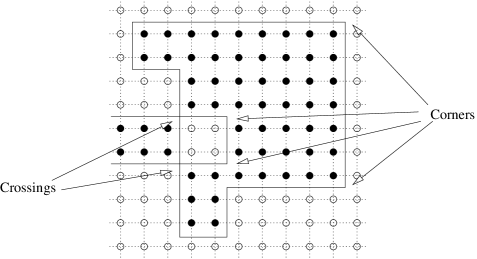
Figure 1: Example of the correspondence between spins and loops. All the energy is concentrated in the corners and crossings of the loops.

By looking at the energy of the loop model it is not difficult to see that it can be written as $E=n_{2}+4\kappa n_{4}$, where $n_{2}$ is the number of bending points of the loops formed by the interface, and $n_{4}$ is the number of self-crossings. That means that $\kappa\to 0$ is the limit for the non-self-avoiding loops, and the $\kappa\to\infty$ is the completely-self-avoiding limit, in which no crossing of loops can exist. Thus the system likes flat interfaces. This is the main reason for the creation of energy barriers while cooling. The system tends to flatten its interface at a first stage, but this process favors configurations where square domains of any size appear, and at low temperature those configurations are very stable.

In the next section we review the main thermodynamical features of the model. Section 3 is dedicated to a numerical study of the dynamics of this models at low temperature in order to determine whether there is glassy behavior in the 2 dimensional gonihedric model as it is actually the case in the 3 dimensional one. In Section 4 we carry out an analytical study of the behavior of the system at low temperatures and long times that we then proceed to compare to a numerical analysis. Our conclusions are collected in section 5. We relegate some technical details to two appendices.

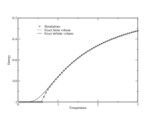
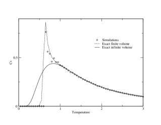
Figure 2: (a) Energy function and (b) specific heat of the system for $\kappa=0$. The exact function at infinite volume, at finite volume, and the Monte-Carlo simulations are plotted.

2 Thermodynamics of the model

Let us begin with the simplest case $\kappa=0$ that is exactly solvable in the infinite volume limit and can be reduced to an easy-computable sum for finite volume (see appendix A). The exact solution for the model with $\kappa=0$ [18] shows that there is no phase transition at finite temperature. If we take a look at fig.2 we will see the infinite volume energy function and specific heat compared to the numerical results and to the exact finite volume calculation. All discrepancies between simulations and the infinite volume calculations are due to finite volume effects as we can see comparing the simulations with the exact finite volume calculations.

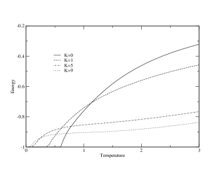
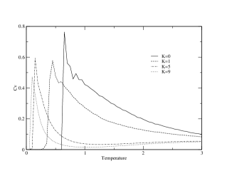
Figure 3: (a) Energy function and (b) specific heat of the system for different values of $\kappa$. Only simulations are plotted. Signals of the non-monotonic behavior can be seen for the $\kappa=5$ and $\kappa=9$ case in the high temperature region of the plot.

For the other case with $\kappa\neq 0$ there is no exact infinite volume solution or easy-computable finite-volume expression, but the simulations do not show marked differences with the $\kappa=0$ case, so we are forced to conclude that there is no ordered phase at low temperature (see fig.3). The maximum in the specific heat seen in the $\kappa=0$ case is still present at the same point (as it should, because it reveals the temperature where the first excitations appear in the bulk) and behaves in the same way. The only remarkable difference is the appearance of a second structure for sufficiently large $\kappa$ (An indication for this can be seen in fig.3b in the non-monotonic behavior of the specific heat for $\kappa=5$ and $9$. Notice the rescaling of the data mentioned in the footnote). This second structure can be interpreted as the appearance of a new state for the plaquette variables whose energy grows with $\kappa$. No volume dependence of this structure has been found, so there is no evidence of phase transition. In figures 4a and 4b we can actually see the formation of this secondary structure and its independence on the volume, respectively.

Figure 4: Closer look to the secondary structure. In (a) there is the evolution of the structure with $\kappa$. Remember that all the data has been rescaled to make the comparison between them easier. In (b) the dependence of this structure with the volume is tested for $\kappa=9$. The conclusion is that it is not dependent on the volume.

The same model but in 3 dimensions exhibits a quite complex phase space, with a thermodynamical transition at a temperature $T_{c}$ between two distinct phases that happens to change from first order to second order when the value of $\kappa$ crosses some critical value [6]. Also a dynamical transition is present in the 3 dimensional model at a temperature $T_{g}\leq T_{c}$.

The fact that there is no phase transition in this spin model can be eventually traced back to the fine tuning of the parameters in the Hamiltonian. Since there is only one phase, no useful order parameter can be constructed. This makes impossible the analysis of the dynamics of this model along the conventional lines of domain growth used in [15]. The dynamical properties of this 2D model will be discussed in the next section.

3 Dynamical analysis of the model

As we have mentioned above our motivation in studying this model is to determine if the dynamical behavior that it exhibits glassy features, as its 3D counterpart, or just signs of very slow evolution. The technique we shall use in this section will be based on two-time correlation functions [16, 17]. Before entering into details let us stop for a moment to understand which are the main features of the evolution of the system.

3.1 Thinking about dynamics

For this qualitative analysis we are going to use the loop language. As we have seen, all the energy is concentrated in the corners of the loop and in the crossing of one loop with each other. To simplify the reasoning we are going to use the $\kappa=0$ limit where the loops can freely cross each other, but the same conclusions can be obtained with $\kappa\neq 0$. We are going to study the evolution at low temperatures, so we have to accept that thermal fluctuations are rare.

Figure 5: Examples of loop configurations. (a) A disordered one, before evolution takes place. (b) After some evolution the loops have reduced the number of corners and have found a metastable configuration.

A disordered configuration (fig.5(a)) will try to evolve by straightening the boundaries of the domains in order to minimize the number of corners. After this first thermalization, the system will end up with some long lines glued together with some corners in a non-optimal way (see fig.5(b)). In general, by decreasing the energy in every step, the loop is going to get trapped in some very stable states whose energy cannot decrease further without increasing it temporarily. The first phase of the evolution is really fast due to the fact that almost all moves decrease the energy.

From this point on, the evolution is quite slow because there are energy barriers to jump over that the system has created during the first fast evolution.

3.2 Is there a dynamical transition?

Let us make now a more detailed quantitative analysis of the dynamical behavior of the model. The magnitude we are going to use is the autocorrelation function of the energy per plaquette $e_{i}$

$$C(t,t_{w})=\frac{1}{N}\sum_{i}e_{i}(t_{w})e_{i}(t)\quad,\qquad t>t_{w}$$ (1)

where the sum runs over all the plaquettes in the lattice. To avoid over-counting the bonds, we have taken the following definition for the energy per plaquette. For each plaquette we will count the energy coming from the plaquette term, the two next to nearest neighbor terms, and two of the four nearest neighbor terms in such a way that one bond is horizontal and the other is vertical.

Let us now describe the results from our numerical analysis. All simulations shown here have been performed with a metropolis-like Monte Carlo algorithm with periodic boundary conditions. The volume is $100^{2}$ in all the data, unless otherwise indicated. The data presented in this section correspond to averaging over 25 independent systems.

We start by studying two different waiting times like for example $t_{w}=100,1000$ and a few temperatures. We can easily see that there are some temperatures where the autocorrelation function $C(t,t_{w})$ depends only on $t-t_{w}$, a good indication that the system has reached equilibrium (unlike for instance in a glassy phase), while at lower temperatures the autocorrelation function happens to depend on $t$ and $t_{w}$ independently. In figure 6 we can see an example of this.

Figure 6: Autocorrelation function for different temperatures. (a) At this temperatures the autocorrelation function depends only on $t-t_{w}$. The fits to the data are plotted with lines. (b) At these lower temperatures the autocorrelation looks dependent of $t_{w}$ and $t$ independently.

This behavior could hint to the existence of some kind of dynamical transition like the same model in 3D. To make it clearer we can look at the form of the autocorrelation function above $T^{*}$, where the supposed dynamical transition would take place. We can attempt a fit to this data with an stretched exponential

$$A\exp\bigg{[}-\bigg{(}\frac{t-t_{w}}{\tau}\bigg{)}^{c}\bigg{]}$$ (2)

It’s clear from the plots in fig.6a that the fits are apparently very satisfactory.

If we extract $\tau$ from the fits and make a plot as a function of the temperature, we will see that $\tau$ grows when we decrease the temperature. This would suggest that the $\tau$ could diverge at some finite temperature, so we try to fit it with a power-like divergence function. The fitting function we have used is

$$\frac{K}{(T-T^{*})^{b}}$$ (3)

The fit is shown in figure 8 (solid curve), and it provides a value for $T^{*}$. The problem is that the value the fit delivers is around $0.57$, while looking at fig.(6) we expected something between 0.8 and 0.9, exactly where we are beginning to see $t_{w}$ dependence. The procedure is thus not self-consistent and we need some explanation for this discrepancy.

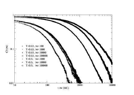
Figure 7: Exploring longer waiting times $t_{w}$ we can see the slow approximation to equilibrium of the autocorrelation function. Two different temperatures are plotted. In the lower temperature ($T=0.5$) the equilibrium is not yet reached, but the range where the dependence in $t_{w}$ is not manifest grows with $t_{w}$.

Let’s explore much longer waiting times. If we do that, we will be able to understand exactly what is happening. In figure 7 we discover that at longer waiting times the dependence in $t_{w}$ disappears, leaving only a function of $t-t_{w}$. This is an indication that the system is not in a putative glassy phase but is just exhibiting an extremely slow relaxation to equilibrium.

Once we have reached the equilibrium at lower temperatures we can fit and extract the autocorrelation time. Adding this new data to the $\tau$ vs. temperature plot we realize that the previous fit is not satisfactory with this new data, so we are lead to make a new fit. After this new fit with more data is performed, the new value for $T^{*}$ happens to be much lower than the previous estimation (see fig. 8, doted curve).The new value of $T^{*}$

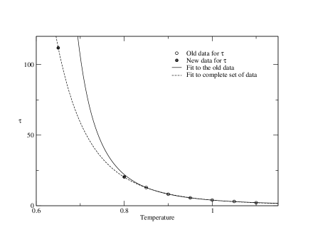
Figure 8: New data and new fit of the autocorrelation time in terms of temperature.

decreases to $0.29$. Thus supposing that we can go on equilibrating the system at any temperature for large but finite values of $t_{w}$, we must conclude that the $T^{*}$ parameter will get closer to zero with each new point we include in the data. We conclude that there is no dynamical transition to a glassy phase, even though that was the case in the 3 dimensional version of the model.

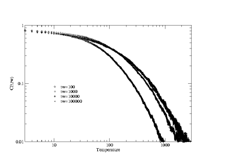
Figure 9: Example for $\kappa=9$ of the approximation to the equilibrium of the autocorrelation function at temperature $T=0.7$

The autocorrelation function at low temperatures depends on $t_{w}$ but when we increase the value of $t_{w}$ this dependence disappears completely. In this example the two last sets of data for $T=0.65$ coincide, so we can declare that it is independent of $t_{w}$ for $t_{w}>10^{4}$ (at this temperature). We have not reached the complete equilibrium in the $T=0.5$ case, but we can see that for $t_{w}=10^{4}$ and $t_{w}=10^{5}$ the coincidence has grown considerably. So the conclusion is that the autocorrelation is approximating to some equilibrium shape. For $\kappa\neq 0$ the analysis follows exactly the same steps, and the same conclusion is reached. We can see in fig.9 that the same kind of behavior is present in $\kappa=9$.

We can take a look at other observables like the two time overlap function $Q(t_{w}+t,t_{w}+t^{\prime})$, or the autocorrelation of the local magnetization $C_{m}(t_{w}+t,t_{w})$ [17]. Suppose we let a system evolve through a time $t_{w}$, then we make two copies of the system and evolve them independently $t$ and $t^{\prime}$ respectively, then the observables are defined as

$$Q(t_{w}+t,t_{w}+t^{\prime}) = \frac{1}{N}\sum_{i}\sigma^{(1)}_{i}(t_{w}+t)\sigma^{(2)}_{i}(t_{w}+t^{\prime})$$ (4)

$$\qquad C_{m}(t_{w}+t,t_{w}) = \frac{1}{N}\sum_{i}\sigma_{i}(t_{w})\sigma_{i}(t_{w}+t)$$ (5)

where the upper-index indicates which is the copy that the spin belongs to.

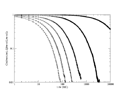
Figure 10: The autocorrelation function of the local magnetization $C_{m}(t_{w}+t,t_{w})$ (Symbols) and the overlap function $Q(t_{w}+t/2,t_{w}+t/2)$ (lines). Lines are $C_{m}$ and symbols are $Q$ data. From left to right, $T=1.1$($\bigcirc$), $T=1.0$($\square$), $T=0.9$($\Diamond$), $T=0.8$($\triangle$), $T=0.65$(+), $T=0.5$($\times$). Formula (6) is clearly verified.

In equilibrium (that is when the autocorrelation is independent of $t_{w}$) they should satisfy

$$Q(t_{w}+t,t_{w}+t)=C_{m}(t_{w}+2t,t_{w}).$$ (6)

We can see in figure 10 that the relation (6) is fully accomplished by our system. Another indication of the non-glassiness of our model (for $\kappa=0$ in this case). The same behavior is present in $\kappa\neq 0$.

4 Analytical results for the evolution

One of the differences between glassy and non-glassy evolution is the fact that for the former, logarithmic growth of domains dominates the evolution of the system at long times. Then we are used to talk in terms of domains and domain walls, velocity of the domain growth, or the energy contained in a domain wall.

The reason that the domain growth concepts cannot be applied to the gonihedric model in 2 dimensions, unlike traditional Ising-type models, is that there is no good local order parameter that allows us to say when a piece of ‘ordered’ system is in one ground-state or the other, so we cannot distinguish domains with different ground-state configuration in its bulk.

In the gonihedric spin model there are so many different ground states that we can travel around a plaquette without crossing any extra accumulation of energy, and yet find extra energy in the plaquette we have been surrounding. This would not be possible if a domain wall would have existed. Here rather than domains we have to talk about point-like defects. In figure 11 we can see an example for $\kappa=0$ and for $\kappa\neq 0$ where an isolated defect (accumulation of energy) is marked with a big $\times$.

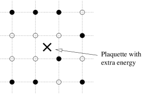
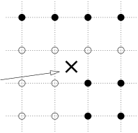
Figure 11: Examples of isolated defects for (a) $\kappa=0$ and (b) $\kappa\neq 0$

4.1 Defect dynamics at very long times

From now we are going to consider the case $\kappa=0$. Already in [13] Buhot and Garrahan defined the dual version of the gonihedric model we are going to use in this section. This duality is just a change of variables, from spins to plaquette variables, where the plaquette variable can be defined in the way

$$\tau_{[i,j,k,l]}=\frac{1-(\sigma_{i}\sigma_{j}\sigma_{k}\sigma_{l})}{2}$$ (7)

i.e., the plaquette dual variable is zero when there is no extra energy accumulated on it and is equal to $+1$ when there is a defect there. Then the extra energy of the system will be just the sum of the $\tau$ variables, or the number of defects.

But the dual model is not just a model of defects. The fact that the defects are defined in terms of spin configurations of an interacting spin model is essential, and provides the defect model an special constrained dynamics. There are some rules in order to move, create or annihilate defects: One defect on its own can’t move, it is stable as it is, the only way it can move is through the creation of two more defects, that means to climb up an energy barrier $\Delta E=2$. In contrast, two neighboring defects can freely move, but only in one direction (horizontal pairs move vertically and vertical pairs move horizontally). The only way defects can disappear is by meeting four defects in a square pattern, or when a moving pair collides with an isolated defect, then the moving pair will disappear moving the isolated defect as a result. This description in terms of moving defects will allow us to find an analytical expression for the energy decay at very long times.

The energy is related with the number of defects as we mentioned before, so we would like to know how defect density evolve in time. To do that we need to understand which is the leading mechanism that make defects disappear.

Our starting point will be a system that has relaxed from a disordered configuration to a low temperature for a long time. So at that moment we have to consider that all the defects are isolated. In these conditions, the movement of all those defects is really slow, because to move they have to create a pair of defects, i.e. overcome an energy barrier. The probability to do this is $\sim\exp(-2/T)$, where $T$ is the temperature. The characteristic time will this be $\sim\exp(2/T)$. For low temperatures, this will be very long time, and we can neglect the possibility of two pairs of defects being created successively.

Let us assume that a pair of defects has been created (see the first diagram of Fig. 12). After this creation, two defects will move freely in horizontal or vertical direction. Because the move of the pair is much faster than the creation of the next pair, the process may conclude in two ways: either the pair returns to the defect it just left behind and returns to the original configuration, or it finds in its random-walk-like movement another defect, collides with it, and disappears, resulting in a move for the secondary defect too. The first case leaves the final configuration unchanged so it represents a frustrated trial of moving an isolated defect, while the second ends up with two defects displaced by one lattice step. In figure 12 there is an sketch of that process.

Figure 12: Sketch of the leading process that allows defects to move. In the first step an isolated defect transforms in three complementary defects, then two of them move in a random walk like way until they find a second defect to combine and disappear.

Thus as we are not sure that creating that extra pair is going to provide a move of the defect because of the frustrated trials, we cannot compute the average time for the traveling pairs of defects to reach a given distance $d$. In fact this average is divergent. We have to compute instead the probability of a success in colliding with a different defect once a pair is created. The inverse of this probability will give to us (by the same argument as before) the characteristic time for the successful move to happen.

The probability of creating a pair is already known and is $\sim\exp(-2/T)$, the probability of a successful move of the pair i.e. reaching another defect, can be easily determined by considering a random walk with an absorbing wall at the origin, and computing the probability of arriving at a distance $d$ for the first time [19]. Some details are given in Appendix B. The result is $1/d$. Thus the final probability for an isolated defect to move one step is

$$\mathcal{P}\sim\frac{\exp(-2/T)}{d}$$ (8)

But the distance $d$ can be parameterized in terms of the density of defects $\rho$ like $d\sim 1/\rho$ so

$$\mathcal{P}\sim\rho\exp(-2/T)$$ (9)

and clearly the number of MC steps needed to move one site a given defect is

$$\tau_{1}\sim\mathcal{P}^{-1}\sim\frac{\exp(2/T)}{\rho}$$ (10)

Now, we know the probability of an isolated defect to move one step in the lattice. The next thing we need to know is how often two defects meet each other and become a pair. This is interesting because once they become a pair they will move freely and will easily find a third defect to decay with. Only at this point and not before we have decreased in two units the number of defects. Let’s do the calculation.

As the move of a pair is very fast, we only need to know the time needed for one defect to meet another one. The move of defects is a slow random walk with a characteristic time click $\tau_{1}$. Unlike in the previous case the probability of one defect meeting another one is $1$, and the characteristic time needed to travel a distance $d$ will be proportional to $d^{2}$, so finally the characteristic time $\tau$ needed for two defects to meet is

$$\tau\sim\tau_{1}\bigg{(}\frac{1}{\rho}\bigg{)}^{2}\sim\frac{\exp(2/T)}{\rho^{3}}$$ (11)

Now we can set the differential equation of the evolution of the number of defects

$$\frac{\textrm{d}\rho}{\textrm{d}t}\sim\frac{-2}{\tau}\rho\sim-2\rho^{4}\exp(-2/T)$$ (12)

This differential equation is valid only for low temperatures and long times (because there are only isolated defects), and low density of defects (because we considered large distances between defects), but this condition is implicit if we demand low temperatures and very long times.

Solving (12) we find that the density of defects should evolve in time like $\rho\sim t^{-\frac{1}{3}}$ and as a consequence the energy evolves in the same way. In the next section we are going to perform a simulation of the energy at very long times and compare the way it evolves with our prediction.

4.2 Long times simulation

To compare with the analytical result we performed long simulations at very low temperatures. For this purpose we started with a disordered initial configuration and let it evolve with a Monte Carlo algorithm at very low temperatures like $0.4$ or $0.33$. The final data is the average of 20 independent evolutions from 20 different initial states.

In figure 13 we can see the evolution in time of the defect concentration, closely related to the energy density through the relation $\rho=(E+1)/2$ where the energy density is defined here as $E=-\frac{1}{N}\sum_{i}(\sigma\sigma\sigma\sigma)_{\Box_{i}}$

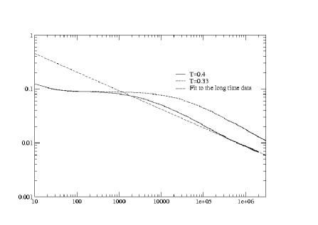
Figure 13: Defect concentration in function of time in a log-log plot. The slope at the latest stage of evolutions around 0.34 for $T=0.4$.

The plateau starts when [13] the system has already reached an stable configuration and finds energy barriers that makes difficult to decrease the energy. As we have seen before those energy barriers cost an energy $\Delta E=2$, so the time needed to reactivate the evolution will be of order $\sim\exp(2/T)$. After the plateau the evolution contains only isolated defects and spontaneous fluctuations in form of pairs of defects that appear when an isolated defect is trying to move. So this should be the range of validity of our calculation, or in other words, in this region the evolution should be like $\rho\sim t^{-\frac{1}{3}}$. Note that this behavior should set in rather slowly (see AppendixB) and therefore it should be apparent only for very low concentration of defects. Note also that the evolution depends only on the concentration of defects once we are in the activated regime.

Indeed when we look at plot of the data (see fig.13) it is clear that in the activated regime in a logarithmic scale, the behavior is approximately linear. However the slope changes slightly with the concentration of defects, which we understand as a signal of the slow setting in of the asymptotic regime which we just discussed. At this very late stage (beyond $\sim 5\times 10^{5}$ Monte-Carlo steps for $T=0.4$) the slope stabilizes to a value close to $-0.34$; that is really close to the one we predicted. Note that the bulk of the data lies precisely in this region (for this temperature we have run up to $2\times 10^{6}$). For $T=0.33$ we have not yet reached the region where the fit of the slope becomes stable, in spite of having run up to $3\times 10^{6}$ sweeps; however we have compared the slopes at similar values of the concentration of defects with the $T=0.4$ case and found quite similar values. From this we conclude that for enough long times we would obtain a value for the slope compatible with the $-0.33$ we expect.

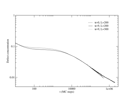
Figure 14: Defect concentration in function of time in a log-log plot for $T=0.4$. Two different volumes for $\kappa=9$ and one for $\kappa=0$ are compared.

For $\kappa\neq 0$ it is harder to know exactly what is the law for the evolution of the defects at long times and low temperatures. Some simulations have been made. In figure 14 we compare a long time simulation of $\kappa=0$ and $\kappa=9$. It can be seen that the $\kappa=9$ case does not seem to follows a power law (two different volumes for $\kappa=9$ are shown to reflect that the plot is volume independent). At very long times the evolution, though rather similar, it is actually faster, since the defect concentration is reaching lower values in shorter times. This is expected due to the lack of a pure geometrical interpretation in the $\kappa\neq 0$.

5 Conclusions

In this work we have analyzed the dynamical behavior of a two dimensional spin model with very ‘geometric’ couplings. The microscopic surface tension is zero and the energy is concentrated on the corners of the loops separating regions of different ferromagnetic states (ferromagnetic states are not the only ground states, the degeneracy of the ground state is $2^{2\ell}$ or $2^{\ell}$ depending on whether the self-avoidance parameter $\kappa$ is turned on or not).

The model has rather trivial thermodynamic properties for non self-avoiding loops. It can actually be mapped to an exactly solvable six-vertex model, albeit exhibiting rather remarkable finite size effects. When the self-avoidance parameter is turned on, no phase transition or thermodynamic singularity is found.

On the contrary, the dynamical properties of the system are rather interesting. Its 3D counterpart does exhibit logarithmic growth of domains and quite clear glassy behavior below a certain temperature. We do find slow dynamics, but they rather correspond to a power law ($\kappa=0$) or faster ($\kappa\neq 0$), and definitely there is no sign of glassy dynamics —at least down to the rather low temperatures we have explored.

Appendix A The 2D finite size partition function for $\kappa=0$

The partition function for our model with $\kappa=0$ is,

$$\mathcal{Z}=\sum_{\{\sigma\}}e^{-\beta{\mathcal{H}}_{\kappa=0}}$$ (13)

where $\{\sigma\}$ is the set of all possible configurations of spins, and ${\mathcal{H}}_{\kappa=0}$ is the $\kappa=0$ rescaled Hamiltonian

$${\mathcal{H}}=-\sum_{[i,j,k,l]}\sigma_{i}\sigma_{j}\sigma_{k}\sigma_{l}=-\sum_{\Box}\sigma\sigma\sigma\sigma$$ (14)

the last step just being a simpler form of writing the Hamiltonian, with the notation $\Box$ meaning spins forming a plaquette in the lattice.

We can transform the expression (13) in the following way

$$\mathcal{Z}=\sum_{\{\sigma\}}e^{-\beta{\mathcal{H}}}=\sum_{\{\sigma\}}\prod_{\Box}e^{\beta\sigma\sigma\sigma\sigma}$$ (15)

$$\quad=(\cosh(\beta))^{N}\sum_{\{\sigma\}}\prod_{\Box}\Big{\{}1+x\,\sigma\sigma\sigma\sigma\Big{\}}$$ (16)

where $x\equiv\tanh(\beta)$ Expanding the product and performing the summation over configurations only terms with an even power on each spin will survive. It’s not difficult to see that this summation can be mapped into another combinatorial problem.

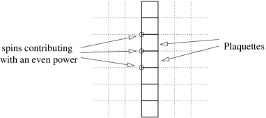
Figure 15: one column of plaquettes. Each spin appears 2 times so this term contributes to the sum with a weight $x^{\ell}$.

Consider that we have a term that contains one plaquette. This term will not contribute unless some of the plaquettes beside it appear also in that term. We have two ways to make this term contribute, either we take also the plaquettes above and below it or the plaquettes at the right side and the left side. In any case we still have problems with four spins (two spins of each new plaquette), so if we continue adding plaquettes in the same direction we will complete a vertical row of plaquettes or an horizontal one (see fig.15) with the help of the boundary conditions. That means that the simplest combination of plaquettes that is going to contribute to the summation will be a column or an horizontal line of plaquettes, and its weight will be $x^{\ell}$ where $\ell$ is the length of the row ($N=\ell^{2}$)

Then we have to count all possible combinations of vertical and horizontal lines, multiplying their weights. Only two more things have to be taken into account. When a term contains horizontal and vertical lines some plaquettes have to be removed because if not their spins would have an odd power (see fig.16). The plaquettes that we have to remove are the ones on the crossings of vertical and horizontal lines. Finally an overall $1/2$ factor has to be used to compensate the over-counting, because each spin configuration has two possible representations in this combinatorial problem.

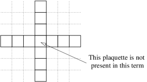
Figure 16: An example of a term with vertical and horizontal lines. This term contributes with a weight $x^{2\ell-2}$.

All this has been made to transform the expression

$$\sum_{\{\sigma\}}\prod_{\Box}\Big{\{}1+\sigma\sigma\sigma\sigma x\Big{\}}$$ (17)

in

$$2^{N}\frac{1}{2}\sum_{v=0}^{\ell}\sum_{h=0}^{\ell}\binom{\ell}{v}\binom{\ell}{h}x^{\ell(h+v)-2hv}$$ (18)

that is much more simple at least in the computational sense. The combinatorial factor $\binom{\ell}{v}$ is the number of different configurations for $v$ vertical columns of plaquettes, and the same for the horizontal. Working a little bit more we can simplify this expression one step further performing one of the summations and find its final form

$$\mathcal{Z}_{\ell}=(2\cosh(\beta))^{N}\frac{1}{2}\sum_{v=0}^{\ell}\binom{\ell}{v}\Big{[}x^{v}+x^{\ell-v}\Big{]}^{\ell}$$ (19)

where is now clear the over-counting if you realize that each term is invariant under $v\to\ell-v$.

Now this expression can be calculated easily at any temperature with a computer for any square lattice. Also in the limit $\ell\to\infty$ we can calculate exactly the sum in (19) (which is equal $2$ for any temperature different from zero) and recover the exact expression for the infinite volume partition function

$$\mathcal{Z}_{\infty}=(2\cosh(\beta))^{N}$$ (20)

Now from this expressions for the partition functions we can extract information like the energy or the specific heat that we plot in section 2.

Appendix B Probability of a pair of defects meeting a third one

The magnitude we want to calculate is the probability for a pair of defects following a random walk with an absorving wall at $x=0$ to reach a distance $x$, where the pair is absorbed, starting at point $x_{0}$. We call this probability $f_{n}$. In the asymptotic limit where the number of random walk steps $n$ is large, the probability of traveling from $x_{0}$ to $x$ in $n$ steps is

$$Q_{n}^{0}(x,x_{0})=\frac{e^{-(x-x_{0})^{2}/2n}}{(2\pi n)^{1/2}}.$$ (21)

The index zero denotes that this is an unrestricted random walk. Now we need to find the probability of going from $x_{0}$ to $x$ in $n$ steps with an absorbing wall at the origin. We shall use the method of images in order to subtract the random walks that are forbidden because of the wall with an auxiliary walker that starts his walk at position $-x_{0}$. The probability we are interested in is

$$Q_{n}^{W}(x,x_{0})=Q_{n}^{0}(x,x_{0})-Q_{n}^{0}(x,-x_{0})$$ (22)

To take into account that the pair is absorved at point $x$, we have to exclude random paths where $x$ is visited more than once. Let the generating function for the probabilities $Q_{n}^{W}(x,x_{0})$ be

$$\mathcal{P}(z)=\sum_{n=1}^{\infty}Q_{n}^{W}(x,x_{0})z^{n}=\sum_{n=1}^{\infty}p_{n}z^{n}$$ (23)

and consider the generating function of the probabilities $Q_{n}^{W}(x,x)$

$$\mathcal{R}(z)=\sum_{n=1}^{\infty}Q_{n}^{W}(x,x)z^{n}=\sum_{n=1}^{\infty}r_{n}z^{n}$$ (24)

The probability we have after $f_{n}$ obeys the relation

$$p_{n}=f_{n}+f_{n-1}r_{1}+f_{n-2}r_{2}+\cdots+f_{1}r_{n-1}$$ (25)

or, in terms of generating functions,

$$\mathcal{F}(z)=\frac{\mathcal{P}(z)}{\mathcal{R}(z)}$$ (26)

Finally,

$$\mathcal{P}(z)=\frac{e^{-x\sqrt{2y}}}{\sqrt{2y}}[e^{x_{0}\sqrt{2y}}-e^{-x_{0}\sqrt{2y}}],$$ (27)

$$\mathcal{R}(z)=\frac{1}{\sqrt{2y}}[1-e^{-2\sqrt{2y}}],$$ (28)

where we have taken $z=e^{-y}$, and the condition $z<1$ is needed to perform the integrations. From these two results and eq.26,

$$\mathcal{F}(z)=\frac{\mathrm{sinh}x_{0}\sqrt{2y}}{\mathrm{sinh}x\sqrt{2y}}$$ (29)

This generating function evaluated at the particular point $z=1^{-}$ gives us the desired probability

$$\sum_{n=1}^{\infty}f_{n}=\mathcal{F}(1^{-})=\frac{x_{0}}{x}.$$ (30)

References

-
[1]
R.V: Ambartzumian, G.S. Sukasian, G.K. Savvidy and K.G. Savvidy, Phys. Lett. B275 (1992) 99;
G.K. Savvidy and K.G. Savvidy, Int. J. Mod. Phys. A8 (1993) 3393;
G.K. Savvidy and K.G. Savvidy, Mod. Phys. Lett. A8 (1993) 2963. -
[2]
G.K. Savvidy and F.J. Wegner, Nucl. Phys. B413 (1994) 605;
G.K. Savvidy and K.G. Savvidy, Phys. Lett. B324 (1994) 72;
G.K. Savvidy, K.G. Savvidy and F.J. Wegner, Nucl. Phys. B443 (1995) 565;
J. Ambjorn, G. Koutsoumbas and G.K. Savvidy, Europhys.Lett. 46 (1999) 319 (cond-mat/9810271). - [3] G.K.Savvidy, The system with exponentially degenerate vacuum state (cond-mat/0003220).
- [4] G. Koutsoumbas and G.K. Savvidy, Three–dimensional gonihedric spin system Mod.Phys.Lett. A17 (2002) 751 (cond-mat/0111590).
- [5] G. Koutsoumbas, G.K. Savvidy and K.G. Savvidy, Phys.Lett. B410 (1997) 241 (hep-th/9706173).
-
[6]
M. Baig, D.Espriu, D. Johnston and R.P.K.C. Malmini,
J.Phys. A30 (1997) 7695
(hep-lat/9703008).
D.Espriu, M. Baig, D.A.Johnston, R.K.P.C.Malmini, J.Phys. A30 (1997) 405 (hep-lat/9607002). - [7] D.A. Johnston and R.P.K. Malmini, Phys.Lett. B378 (1996) 87, (hep-lat/9508026).
- [8] A.Lipowski, D.Johnston and D.Espriu, Phys.Rev. E62 (2000) 3404 (cond-mat/0004466).
- [9] M.R. Swift, H. Bokil, R.D.M. Travasso and A.J. Bray, Phys.Rev. B62 11494 (2000) (cond-mat/0003384).
- [10] A. Lipowski, J. Phys. A30 (1997) 7365.
-
[11]
A. Lipowski and D. Johnston, J.Phys. A33, 4451 (2000)
(cond-mat/9812098).
A. Lipowski and D. Johnston, Phys.Rev. E61, 6375 (2000)(cond-mat/9910370).
A. Lipowski and D. Johnston, Phys.Rev. E64, 041605 (2001)(cond-mat/0105602). - [12] P. Dimopoulos, D. Espriu, E. Jane, A. Prats. Phys.Rev.E 66:056112, 2002. (cond-mat/0204403)
- [13] A. Buhot, J.P.Garrahan, Phys. Rev. Lett. 88, 225702, (2002)(cond-mat/0111035)
- [14] J.D. shore, M. Holzer, J.P.Sethna, Phys.rev. B46 11376, (1992)
- [15] Z. W. Lai, G. F. Mazenco, Phys.Rev. B37 9481, (1988)
- [16] D. Alvarez, S.Franz, F.Ritort, Phys.Rev. B54 9756, (1996)
- [17] A. Barrat, R. Burioni, M.M zard, J. Phys. A29 (1996) 1311 (cond-mat/9509142)
- [18] R. J. Baxter, Exactly Solved Models in Statistical Mechanics (Academic Press, London, 1982)
- [19] M. E. Fisher Walks, Walls, Wetting & Melting J.Stat.Phys. 34 667 (1984)