The anisotropic conductivity of two-dimensional electrons on a half-filled high Landau level

Abstract

We study the conductivity of two-dimensional interacting electrons on the half-filled $N$th Landau level with $N\gg 1$ in the presence of the quenched disorder. The existence of the unidirectional charge-density wave state at temperature $T<T_{c}$, where $T_{c}$ is the transition temperature, leads to the anisotropic conductivity tensor. We find that the leading anisotropic corrections are proportional to $(T_{c}-T)/T_{c}$ just below the transition in accordance with the experimental findings. Above $T_{c}$ the correlations corresponding to the unidirectional charge-density wave state below $T_{c}$ result in the corrections to the conductivity proportional to $\sqrt{T_{c}/(T-T_{c})}$.

1. Introduction. Two-dimensional electrons in a perpendicular magnetic field was a subject of intensive studies, both theoretical and experimental, for several decades AFS ; QHE . It has been found that the properties of two-dimensional electrons in the magnetic field are strongly affected by the presence of electron-electron interaction as well as by impurities. The behaviour of the system in a strong magnetic field where only the lowest Landau level is occupied has been investigated in great details QHE . But only several attempts were made to consider the system in a weak magnetic field (large number of Landau levels $N\gg 1$ are occupied) where the Coulomb energy at distances of the order of the magnetic length exceeds the cyclotron energy Attempts .

The progress in understanding the clean two-dimensional electrons in a weak magnetic field was achieved by Aleiner and Glazman who, by using the small parameter $1/N\ll 1$, have derived the successive theory that describes electrons on the partially filled $N$th Landau level  AG . By treating the effective electron-electron interaction on the $N$th Landau level within the Hartree-Fock approximation, Koulakov, Fogler, and Shklovskii KFS predicted a unidirectional charge-density-wave (UCDW) state (stripe phase) for the half-filled high Landau level at zero temperature and in the absence of disorder. Moessner and Chalker MC showed the existence of the UCDW state on the half-filled high Landau level without disorder below some temperature $T_{0}$. In the presence of disorder the UCDW state on the half-filled high Landau level can exist if the Landau level broadening $1/2\tau$ does not exceed the critical value $1/2\tau_{c}=4T_{0}/\pi$ Burm1 (see Fig. 1). (We use the system of units with $\hbar=1$, $c=1$ and $k_{B}=1$ throughout the Letter.)

The anisotropic magnetoresistance discovered near half-fillings of Landau levels at low temperatures was attributed to the existence of the UCDW state  Exp . This stimulates an extensive study of the properties of two-dimensional electrons in a weak magnetic field Fogler . However up to date, the magnetoresistance of the UCDW state have been theoretically considered in the zero temperature limit only where stripes have well-defined edges Fogler .

The main objective of the present Letter is to present the results for the conductivity tensor of the UCDW state developed on the half-filled high Landau level in the presence of the quenched disorder just below the transition temperature $T_{c}$ where the expansion in the CDW order parameter $\Delta$ is justified.

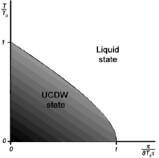
Figure 1: Phase diagram on a half filled high Landau level.

2. UCDW state. The two-dimensional electrons in a weak perpendicular magnetic field $H$ occupy large number ($N\gg 1$) of the Landau levels. We assume that disorder is weak so it leads to the Landau level broadening $1/2\tau$ that satisfies the condition $1/2\tau\ll\omega_{H}$, where $\omega_{H}=eH/m$ is the cyclotron frequency with $e$ and $m$ being the electron charge and the effective electron mass respectively. As the temperature decreases the second-order transition from the homogeneous state to the UCDW state occurs (see Fig. 1). Vector Q that characterizes a period of the UCDW can be oriented along spontaneously chosen direction. Usually, the orientation is fixed either by the intrinsic anisotropy of the crystal or by the small external in-plane magnetic field Fogler . Hereinafter, we assume that the vector Q is directed under angle $\phi$ with respect to the $x$ axis. The period of the UCDW is seemed to be of the order of the cyclotron radius $R_{c}=l_{H}\sqrt{2N+1}$, where $l_{H}=1/\sqrt{m\omega_{H}}$ denotes the magnetic length. More precisely, the modulus of the vector Q equals $Q=r_{0}/R_{c}$, where $r_{0}\approx 2.4$ is the first zero of the zeroth order Bessel function of the first kind $\mathcal{J}_{0}(z)$ KFS ; Burm1 .

The temperature $T_{c}$ of the second-order transition from the homogeneous to UCDW state is determined as the solution of the following equation Burm1 ,

$$\frac{T_{c}}{T_{0}}=\frac{2}{\pi^{2}}\zeta\left(2,\frac{1}{2}+\frac{1}{4\pi T_{c}\tau}\right),$$ (1)

where $\zeta(2,z)$ is the generalized Riemann zeta function and $T_{0}$ the transition temperature in the clean case ($1/\tau=0$). We notice that Eq.(1) has the solution for $T_{c}$ only if the Landau level broadening is smaller than the critical one $1/2\tau\leq 1/2\tau_{c}=4T_{0}/\pi$ as it is shown in Fig. 1. According to Refs. KFS ; MC ,

$$T_{0}=\frac{r_{s}\omega_{H}}{4\pi\sqrt{2}}\left[\ln\Bigl{(}1+\frac{c}{r_{s}}\Bigr{)}-\frac{c}{\sqrt{2}+r_{s}}\right],\quad\frac{1}{N}\ll r_{s}\ll 1$$ (2)

where $c=1/(\sqrt{2}r_{0})\approx 0.3$, and $r_{s}=\sqrt{2}e^{2}/\varepsilon v_{F}\ll 1$ with $v_{F}$ and $\varepsilon$ being the Fermi velocity and the dielectric constant of a media respectively. It is worth mentioning that the $T_{0}$ is determined by the characteristic energy $e^{2}/R_{c}\sim r_{s}\omega_{H}\ll\omega_{H}$ of the screened electron-electron interaction on the $N$th Landau level, cf. Eq.(16).

3. Results. The conductivity tensor $\sigma_{ab}$ of the two-dimensional electrons on the half-filled high Landau level above the transition temperature $T_{c}$, i.e. in the homogeneous state, is known to be isotropic AFS . To this end we show that in the presence of the quenched weak disorder the existence of the UCDW state on the half-filled high Landau level below $T_{c}$ results in the anisotropic corrections to the isotropic conductivity tensor $\sigma_{ab}$. For the temperature slightly below $T_{c}$, where the condition $T_{c}-T\ll T_{c}$ is hold, the anisotropic corrections are given as

$$\left.\begin{array}[]{c}\delta\sigma_{xx}^{(\rm anis)}\\ \delta\sigma_{yy}^{(\rm anis)}\end{array}\right\}=\mp Nf\left(\eta_{c}\right)\mathcal{G}\left(\eta_{c}\right)\cos[2\phi]\frac{T_{c}-T}{T_{c}},$$ (3)

and

$$\left.\begin{array}[]{c}\delta\sigma_{xy}^{(\rm anis)}\\ \delta\sigma_{yx}^{(\rm anis)}\end{array}\right\}=Nf\left(\eta_{c}\right)\mathcal{G}\left(\eta_{c}\right)\sin[2\phi]\frac{T_{c}-T}{T_{c}}.$$ (4)

Here for convenience we introduce the dimensionless parameter $\eta_{c}=1/4\pi T_{c}\tau$ that we use throughout the Letter. The functions $f(z)$ and $g(z)$ are defined as

$$f(z)=\frac{32\mathcal{J}_{1}^{2}(r_{0})z^{3}}{\left(\frac{1}{2}+z\right)^{5}},\,\,g(z)=\frac{16\pi z}{\left(\frac{1}{2}+z\right)\left(z^{2}+\left(\frac{1}{2}+z\right)^{2}\right)},$$ (5)

where $g(z)$ will be used below. The other function $\mathcal{G}(z)$ is given as

$$\mathcal{G}(z)=\frac{\zeta(2,\frac{1}{2}+z)-z\zeta(3,\frac{1}{2}+z)}{-3\zeta(4,\frac{1}{2}+z)+4\Phi_{0}(z)+2\Phi_{2}(z)},$$ (6)

with

$$\Phi_{n}(z)=\frac{\zeta(2,\frac{1}{2}+z)}{z^{2}\mathcal{J}_{0}^{2}(nr_{0})}-\frac{\mathop{\rm Im}\psi(\frac{1}{2}+z+i\,z\mathcal{J}_{0}(nr_{0}))}{z^{3}\mathcal{J}_{0}^{3}(nr_{0})}.$$ (7)

The $\psi(z)$ stands for the digamma function and symbol $\mathop{\rm Im}$ denotes the imaginary part.

There are several features of the main results (3) and (4). First of all, the anisotropic corrections $\delta\sigma_{ab}^{(\rm anis)}$ are proportional to $(T_{c}-T)/T_{c}$. Although, the Eqs.(3) and (4) are derived only for the case of a short-range random potential (quenched disorder), it can be shown that the anisotropic corrections remain proportional to $(T_{c}-T)/T_{c}$ in the case of a long-range random potential as well Burm3 . We emphasize that such temperature dependence of the developing anisotropy in magnetoresistance was observed in the experiments Exp .

The angle dependence of the anisotropic correction (3) to conductivity $\sigma_{xx}$ has the minimum for $\phi=0$, that corresponds to the vector Q directed along the $x$ axis and stripe oriented along the $y$ axis. From Eq.(3) we see that the conductivity $\sigma_{yy}$ along the stripe is enhanced whereas the conductivity $\sigma_{xx}$ across the stripes (along the modulation of the order parameter) is suppressed as it should be according to the experiments Exp . In the same time, the anisotropic correction (4) to $\sigma_{xy}$ vanishes. If the vector Q is oriented at angle $\phi=\pi/4$ with respect to the $x$ axis, the anisotropic correction (3) to $\sigma_{xx}$ becomes zero due to the symmetry between $x$ and $y$ axes. Conversely, the anisotropic correction (4) to $\sigma_{xy}$ is attained the minimum .

The behavior of the anisotropic corrections (3) and (4) as the functions of the parameter $\eta_{c}$ for fixed temperature $T$ and angle $\phi$ are shown in Fig. 2.

In addition, the existence of the UCDW state on the half-filled high Landau level leads to the isotropic correction that for $T_{c}-T\ll T_{c}$ is as follows

$$\delta\sigma_{xx}^{(\rm isot)}=-\frac{N}{\pi}\left[g\left(\eta_{c}\right)+f\left(\eta_{c}\right)\right]\mathcal{G}\left(\eta_{c}\right)\frac{T_{c}-T}{T_{c}}.$$ (8)

The behavior of the isotropic correction (8) as the functions of $\eta_{c}$ for fixed temperature $T$ is shown in Fig. 2.

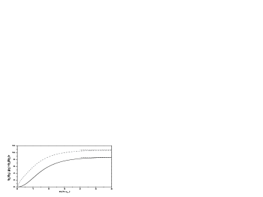
Figure 2: The $f(\eta_{c})\mathcal{G}(\eta_{c})$ and $[g(\eta_{c})+f(\eta_{c})]\mathcal{G}(\eta_{c})/\pi$ as functions of $\ln(1+\eta_{c})$.

4. Model. The grand canonical partition function of the two-dimensional interacting electrons in the random potential $V(\textit{{{r}}})$ subjected to the perpendicular constant magnetic field $H$ and the time-dependent external vector potential A is given by

$$\mathcal{Z}=\int\mathcal{D}[\Psi,\Psi^{\dagger}]\mathcal{D}[V]\,\mathcal{P}[V]\,\exp\mathcal{S}_{0}[\Psi,\Psi^{\dagger},V],$$ (9)

where the action $\mathcal{S}_{0}[\Psi,\Psi^{\dagger},V]$ in the Matsubara representation has the form

$$\mathcal{S}_{0}=\int\limits_{r}\Psi^{\dagger}(\textit{{{r}}})\Bigl{[}i\omega+\mu-\mathcal{H}_{0}+\hat{K}-V(\textit{{{r}}})\Bigr{]}\Psi(\textit{{{r}}})$$ (10)

$$-\frac{T}{2}\int\limits_{rr^{\prime}}\sum_{\alpha\nu_{n}}\Psi^{\dagger}(\textit{{{r}}})I^{\alpha}_{n}\Psi(\textit{{{r}}})\frac{e^{2}}{\varepsilon|\textit{{{r}}}-\textit{{{r}}}^{\prime}|}\Psi^{\dagger}(\textit{{{r}}}^{\prime})I^{\alpha}_{-n}\Psi(\textit{{{r}}}^{\prime}).$$

Here we use the matrix notation $\Psi^{\dagger}(\cdots)\Psi=\Psi^{\dagger\alpha}_{\omega_{n}}(\cdots)^{\alpha\beta}_{nm}\Psi^{\beta}_{\omega_{m}}$ for the electron annihilation $\Psi^{\alpha}_{\omega_{n}}(\textit{{{r}}})$ and creation $\Psi^{\dagger\alpha}_{\omega_{n}}(\textit{{{r}}})$ operators. Superscripts $\alpha,\beta=1,\cdots,2N_{r}$ stands for replica indices combined with spin ones. We introduce the replica indices in order to average over the random potential $V(\textit{{{r}}})$. The subscripts $\omega_{n},\omega_{m}$ denote the Matsubara fermionic frequencies $\omega_{n}=\pi T(2n+1)$. The one-particle hamiltonian $\mathcal{H}_{0}$ for a two-dimensional electron in the presence of the magnetic field $H=\epsilon_{ab}\partial_{a}A^{\rm st}_{b}$ is defined as $\mathcal{H}_{0}=-\textit{{{D}}}^{2}/(2m)$ with the covariant derivative $\textit{{{D}}}=\nabla-ie\textit{{{A}}}^{\rm st}$. The matrix $\omega$ has only diagonal elements $\omega_{nm}^{\alpha\beta}=\omega_{n}\delta^{\alpha\beta}\delta_{nm}$ that represent the Matsubara frequencies $\omega_{n}$. The matrix $I^{\alpha}_{n}$ with elements $(I^{\alpha}_{n})^{\beta\gamma}_{lm}=\delta^{\beta\alpha}\delta^{\gamma\alpha}\delta_{m-l,n}$ is a generator of the $U(1)$ gauge transformation. The time-dependent external vector potential A is involved through the matrix $\hat{K}=\sum_{\alpha,n}K(\nu_{n})I^{\alpha}_{n}$ where

$$K(\nu_{n})=-\frac{e}{m}\textit{{{A}}}(\nu_{n})\textit{{{D}}}+\frac{e^{2}}{2m}\sum_{\nu_{m}}\textit{{{A}}}(\nu_{n-m})\textit{ {{A}}}(\nu_{m}).$$ (11)

Here $\textit{{{A}}}(\nu_{n})$ is the Fourier component of the external vector potential A with frequency $\nu_{n}=2\pi Tn$.

We assume the white-noise distribution for the random potential $V(\textit{{{r}}})$

$$\mathcal{P}[V(\textit{{{r}}})]=\frac{1}{\sqrt{2\pi g}}\,\exp\left[-\frac{1}{2g}\int_{r}V^{2}(\textit{{{r}}})\right].$$ (12)

This distribution corresponds to a short-range random potential with the correlation length $d$ smaller than the magnetic field length $l_{H}$, $d\ll l_{H}$. In high mobility samples used in experiments Exp , however, the disorder potential has long-range correlations. In the case $d\gg l_{H}$ one should distinguish between the Landau level broadening $1/2\tau$ and the inverse transport time $1/\tau_{\rm tr}$. Therefore, the anisotropic (3) and (4) as well as isotropic (8) contributions will be determined by both energy scales $1/\tau$ and $1/\tau_{\rm tr}$ those ratio depends on the value of dimensionless parameter $d/l_{H}$ AFS . Nevertheless, the main result that the anisotropic as well as isotropic corrections to $\sigma_{ab}$ are proportional to $(T_{c}-T)/T_{c}$ will survive for a long-range random potential Burm3 .

5. Method. To proceed we integrate over the random potential $V(\textit{{{r}}})$ in Eq.(9). As usual, it leads to the quartic interaction that we decouple by introducing the matrix field $Q(\textit{{{r}}})$ ELK . The annihilation $\Psi(\textit{{{r}}})$ and creation $\Psi^{\dagger}(\textit{{{r}}})$ operators written in the basis of the eigenfunctions $\phi_{pk}(\textit{{{r}}})$ of the Hamiltonian $\mathcal{H}_{0}$

$$\Psi(\textit{{{r}}})=\sum_{p,k}\psi_{pk}\phi_{pk}(\textit{{{r}}}),\,\,\Psi^{\dagger}(\textit{{{r}}})=\sum_{p,k}\psi_{pk}^{\dagger}\phi_{pk}^{*}(\textit{{{r}}})$$ (13)

involve the electron states on all Landau levels. Therefore, the term with the electron-electron interaction in the action (10) contains the interactions of electrons from different Landau levels. In general, to treat the problem (10) analytically seems to be impossible. However, as it was shown in Ref. AG , if the $N-1$ Landau levels are filled whereas the $N$th Landau level is partially occupied, one can obtain the description of the system in terms of electrons on the $N$th Landau level only provided that the relative strength of the bare Coulomb interaction is small, $r_{s}\ll 1$, and the magnetic field is rather weak, $Nr_{s}\gg 1$.

Following the same strategy as in Ref. Burm2 , we obtain the grand canonical partition function $\mathcal{Z}$ as

$$\mathcal{Z}=\int\mathcal{D}[\Psi,\Psi^{\dagger}]\mathcal{D}[Q]\exp\mathcal{S}[\Psi,\Psi^{\dagger},Q],$$ (14)

where

$$\mathcal{S}=\int\limits_{r}\Psi^{\dagger}(\textit{{{r}}})\Bigl{[}i\omega+\mu-\mathcal{H}_{0}+\hat{K}+iQ\Bigr{]}\Psi(\textit{{{r}}})-\frac{1}{2g}\mathop{\rm Tr}Q^{2}$$

$$-\frac{T}{2}\int\limits_{rr^{\prime}}\sum_{\alpha\nu_{n}}\psi^{\dagger}(\textit{{{r}}})I^{\alpha}_{n}\psi(\textit{{{r}}})U_{\rm scr}(\textit{{{r}}},\textit{{{r}}}^{\prime})\psi^{\dagger}(\textit{{{r}}}^{\prime})I^{\alpha}_{-n}\psi(\textit{{{r}}}^{\prime}).$$ (15)

Here symbol $\mathop{\rm Tr}$ denotes the trace over the Matsubara, replica combined with spin and spatial indices. The electron-electron interaction is written in terms of electron operator $\psi(\textit{{{r}}})=\sum_{k}\psi_{Nk}\phi_{Nk}(\textit{{{r}}})$ on the $N$th Landau level only. The screened interaction $U_{\rm scr}(\textit{{{r}}})$ of electrons on the $N$th Landau level takes into account the effects of electrons on the other levels and has the following form  AG ; Burm2

$$U_{\rm scr}(q)=\frac{2\pi e^{2}}{\varepsilon q}\frac{1}{1+\displaystyle\frac{2\left(1-\frac{\pi}{6\omega_{H}\tau}\right)}{qa_{B}}\left(1-\mathcal{J}_{0}^{2}(qR_{c})\right)}.$$ (16)

It is worth mentioning that the range of the screened electron-electron interaction (16) is determined by the Bohr radius $a_{B}=\varepsilon/me^{2}$. We assume that the magnetic field is so weak that the condition $Nr_{s}^{2}\gg 1$ is hold. That means that the range $a_{B}$ of the screened electron-electron interaction (16) is much less than the magnetic length $l_{H}$. It allows us to treat the interaction in the Hartree-Fock approximation MC .

In the absence of the external vector potential A one can project the first line in Eq.(15) onto the $N$th Landau level, i.e. substitute $\Psi(\textit{{{r}}})\to\psi(\textit{{{r}}})$. Then the action becomes to involve electrons on the $N$th Landau level only and, evidently, it simplifies the analysis. The accuracy of such projection is of the order of $\max\{T,\tau^{-1}\}/\omega_{H}\ll 1$. It is worthwhile to mention that the correction $\pi/6\omega_{H}\tau\ll 1$ in the screened interaction (16) results in the correction of the same order to the $T_{0}$. For reasons to be explained shortly we neglect this effect. However, in order to investigate the response of the system to the external vector potential A such projection onto the $N$th Landau level is not appropriate. We should leave the action (15) as it stands because the matrix elements $D^{a}_{p_{1}p_{2}}=\int_{r}\phi_{p_{1}k}^{*}(\textit{{{r}}})D^{a}\phi_{p_{2}k}(\textit{{{r}}})$ of the covariant derivative $\textit{{{D}}}=(D^{x},D^{y})$ involve the electron states on the adjacent Landau levels. As the last thing we mention that the electrons on the $N$th Landau level should be regarded as spin-polarized according to the numerical findings WS .

The action (15) involves the unitary matrix field $Q(\textit{{{r}}})$. There exists the saddle-point solution $Q(\textit{{{r}}})=W^{-1}U_{\rm sp}W$ in the absence of the electron-electron interaction. Here the constant unitary matrix $W$ describes the global rotation, whereas $(U_{\rm sp})^{\alpha\beta}_{nm}=\delta^{\alpha\beta}\delta_{nm}\mathop{\rm sgn}\omega_{n}/2\tau$ with $1/2\tau=\sqrt{g/2\pi l_{H}^{2}}$. Being motivated by the form of the saddle-point solution we split the matrix field $Q(\textit{{{r}}})$ in transverse $W(\textit{{{r}}})$ and longitudinal $U(\textit{{{r}}})$ components as $Q(\textit{{{r}}})=W^{-1}(\textit{{{r}}})(U_{\rm sp}+U(\textit{{{r}}}))W(\textit{{{r}}})$. As it is well-known the transverse field $W(\textit{{{r}}})$ is responsible for weak localization corrections ELK but in the case of interest they are of the order of $\ln N/N\ll 1$. Therefore we eliminate the transverse field from the future considerations by formally putting $W(\textit{{{r}}})=1$. The transformation of the variable $Q(\textit{{{r}}})$ discussed above leads to the additional measure in the functional integral Pruisken

$$\ln I[U]\sim\int\limits_{r}\sum\limits_{\omega_{n}\omega_{m}}^{\alpha\beta}\left[1-\Theta(nm)\right]U_{nn}^{\alpha\alpha}(\textit{{{r}}})U_{mm}^{\beta\beta}(\textit{{{r}}}),$$ (17)

where $\Theta(x)$ stands for the Heaviside step function.

To describe the UCDW state we introduce the CDW order parameter $\Delta$ that is related with a distortion of the electron density on the $N$th Landau level

$$\langle\delta\rho(\textit{{{q}}})\rangle=2\pi l^{-2}_{H}F_{NN}(\textit{{{q}}})[\delta(\textit{{{q}}}-\textit{{{Q}}})+\delta(\textit{{{q}}}+\textit{{{Q}}})]\Delta,$$ (18)

where the $F_{p_{1}p_{2}}(\textit{{{q}}})$ is defined as

$$F_{p_{1}p_{2}}(\textit{{{q}}})=2\pi l_{H}^{2}\sum\limits_{k}\phi_{p_{1}k}^{*}(0)\phi_{p_{2}k}(\textit{{{q}}}l_{H}^{2})e^{i\frac{1}{2}q_{x}q_{y}l_{H}^{2}}.$$ (19)

In particularly, the form-factor $F_{NN}(q)\approx\mathcal{J}_{0}(qR_{c})$ for $qR_{c}\ll 2N$. The presence of the distortion of the electron density by the charge-density wave on the $N$th Landau level results in the additional periodic potential $\lambda(\textit{{{r}}})$ that is related with the UCDW order parameter as

$$\lambda(\textit{{{q}}})=(4\pi)^{2}T_{0}F_{NN}^{-1}(q)\Bigl{[}\delta(\textit{{{q}}}-\textit{{{Q}}})+\delta(\textit{{{q}}}+\textit{{{Q}}})\Bigr{]}\Delta.$$ (20)

After the Hartree-Fock decoupling FPA of the interaction term in the action (15) and integration over electrons, we obtain

$$\mathcal{Z}\sim\int\mathcal{D}[U]I[U]\exp\mathcal{S}[U],$$ (21)

where the action becomes

$$\mathcal{S}=-\frac{1}{2g}\mathop{\rm Tr}U^{2}+\mathop{\rm Tr}\ln\left(1+(iU+\hat{K}+P_{N}\lambda P_{N})G\right).$$ (22)

The projection operator $P_{N}(\textit{{{r}}},\textit{{{r}}}^{\prime})=\sum_{k}\phi_{Nk}(\textit{{{r}}})\phi_{Nk}^{*}(\textit{{{r}}}^{\prime})$ in the action (22) indicates that the potential $\lambda(\textit{{{r}}})$ exists on the $N$th Landau level only Foot1 . The saddle-point Green function $G^{\alpha\beta}_{nm}(\textit{{{r}}},\textit{{{r}}}^{\prime})$ is determined as

$$G^{\alpha\beta}_{nm}(\textit{{{r}}},\textit{{{r}}}^{\prime})=\delta^{\alpha\beta}\delta_{nm}\sum\limits_{pk}\phi_{pk}^{*}(\textit{{{r}}})\phi_{pk}(\textit{{{r}}}^{\prime})G^{-1}_{p}(\omega_{n}),$$

$$G^{-1}_{p}(\omega_{n})=i\omega_{n}+\omega_{H}(p-N)+i\frac{\mathop{\rm sgn}\omega_{n}}{2\tau},$$ (23)

We notice that the Green function (23) coincides with the Green function averaged over disorder in the self-consistent Born approximation AFS .

6. Conductivity tensor. With the action (22) in hands we can evaluate the contributions to the conductivity tensor $\sigma_{ab}$ due to the presence of the UCDW state on the half-filled Landau level. As one can verify the contributions of the first order in the UCDW induced potential $\lambda(\textit{{{r}}})$ vanish. In order to find the contributions to $\sigma_{ab}$ of the second order in $\lambda$ we should expand the action (22) upto the second order both in $\lambda$ and $K$. Then, integrating over the $U$ fields, we obtain several contributions. We present the diagrams that correspond to them in the standard perturbative technique in Fig. 3.

The first three diagrams (Fig. 3(a)) yield only the isotropic contribution

$$\sigma_{ab}^{(a)}(\nu_{n})=-T\sum\limits_{\omega_{n}}\frac{G_{N}^{3}(\omega_{n})}{1+g\pi^{\omega_{n}}(0,0)}\frac{T_{0}^{2}\Delta^{2}}{(1+g\pi^{\omega_{n}}(0,Q))^{2}}$$

$$\times\frac{4\pi\omega_{H}}{\nu_{n}}\left(\frac{2}{m}\sum\limits_{p}D_{Np}^{a}D_{pN}^{b}G_{p}(\omega_{n}+\nu_{n})-\delta_{ab}\right).$$ (24)

Here the polarization operator $\pi^{\omega_{n}}(\nu_{n},q)$ on the $N$th Landau level is defined as

$$\pi^{\omega_{n}}(\nu_{n},q)=-n_{L}G_{N}(\omega_{n}+\nu_{n})G_{N}(\omega_{n})F^{2}_{NN}(q).$$ (25)

The contribution of diagram Fig. 3(b) is seemed to be proportional to $\mathcal{J}_{0}(r_{0})$ and vanishes therefore. The last diagram Fig. 3(c) is as follows

$$\sigma_{ab}^{(c)}(\nu_{n})=\frac{8\pi\omega_{H}}{\nu_{n}m}T\sum\limits_{\omega_{n}}\frac{G_{N}^{2}(\omega_{n})G^{2}_{N}(\omega_{n}+\nu_{n})T_{0}^{2}\Delta^{2}}{(1+g\pi^{\omega_{n}}(0,Q))^{2}}$$

$$\times\sum\limits_{pp^{\prime}}G_{p}(\omega_{n})G_{p^{\prime}}(\omega_{n}+\nu_{n})\frac{D_{pN}^{a}D_{p^{\prime}N}^{b}I_{NpNp^{\prime}}(\textit{{{Q}}})}{1+g\pi^{\omega_{n}}(0,Q)},$$ (26)

where a single impurity line is written in the Landau level indices representation (see Fig. 4) as

$$I_{p_{1}p_{2}p_{3}p_{4}}(\textit{{{Q}}})=g\int_{q}F_{p_{1}p_{2}}(\textit{{{q}}})F_{p_{3}p_{4}}(-\textit{{{q}}})e^{-i\textit{{{q}}}\textit{{{Q}}}l_{H}^{2}}.$$ (27)

The contribution (26) contains the anisotropic as well as isotropic corrections to $\sigma_{ab}$. If we take $p=p^{\prime}=N\pm 1$ we obtain the anisotropic contribution due to the structure of matrix elements $D_{p_{1}p_{2}}^{a}$. The opposite case $p=N\pm 1$ and $p^{\prime}=N\pm 1$ results in the isotropic correction.

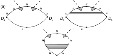
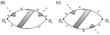
Figure 3: Diagrams for the corrections to $\sigma_{ab}$. The solid lines are the Green functions, the $N/p/p^{\prime}$ symbols denote the Landau level, the dashed lines are the UCDW induced potential $\lambda(\textit{{{r}}})$ and the shaded blocks are impurity ladders.

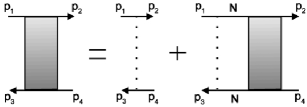
Figure 4: Fig. 4. The equation for the impurity ladder. The frequency $\omega_{n}+\nu_{n}$ runs to the right whereas the $\omega_{n}$ to the left.

Now with a help of the identities $I_{N,N\pm 1,N,N\pm 1}=ge^{\mp 2i\phi}\mathcal{J}_{1}^{2}(r_{0})$ and $I_{N,N\pm 1,N,N\mp 1}=g\mathcal{J}_{1}^{2}(r_{0})$ we perform the summation over the Landau level indices as well as over the Matsubara frequency. As the last step, we express the UCDW order parameter $\Delta$ via the temperature difference $T_{c}-T\ll T_{c}$ as Burm1

$$\Delta=\zeta\left(2,\frac{1}{2}+\eta_{c}\right)\sqrt{\mathcal{G}\left(\eta_{c}\right)}\sqrt{\frac{T_{c}-T}{T_{c}}}$$ (28)

and obtain the results (3),(4) and (8).

7. Fluctuations of the order parameter. The UCDW order parameter $\Delta$ involved in Eq.(22) can be thought of as a saddle-point solution for the plasmon field that appears in the Hubbard-Stratonovich transformation of the screened electron-electron interaction in the action (15). The expansions of physical quantities like free energy and linear response in $\Delta$ is legitimate if we can neglect the fluctuations of the UCDW order parameter $\Delta$. It was shown that they leads to the first order transition at lower temperature $T_{c}-\delta T$ where $\delta T/T_{c}\propto N^{-2/3}$ Burm1 . Therefore, in the considered case of the weak magnetic field ($N\gg 1)$ the effect of the fluctuations on the transition is negligible and the mean-field picture is well justified. There is a legitimate question about the effect of the fluctuations on the conductivity tensor above and below the transition temperature $T_{c}$. Below we consider the former case as more interesting.

At $T>T_{c}$ the mean-field order parameter $\Delta=0$ in average, but the average of its square $\langle\Delta^{2}\rangle$ is non-zero. It leads to the appearance of the corrections to the conductivity tensor $\sigma_{ab}$ above $T_{c}$ due to the presence of the CDW correlations. We can find the contributions of the order parameter fluctuations to $\sigma_{ab}$ by substituting $\langle\Delta^{2}\rangle$ for $\Delta^{2}$ in Eqs.(24) and (26).

Generally, the angle $\phi$ and modulus $Q$ of the CDW vector Q can fluctuate simultaneously foot2 . Naturally, only the isotropic correction can appear in this case. Then, the result for the correction one can obtain from Eq.(8) with a help of the following substitutions

$$\frac{T_{c}-T}{T_{c}}\to\frac{r_{0}}{4\pi N}\sqrt{\frac{T_{c}}{T-T_{c}}},$$ (29)

$$\mathcal{G}\left(z\right)\to\sqrt{\frac{\zeta^{-1}\left(2,\frac{1}{2}+z\right)}{\gamma\zeta\left(2,\frac{1}{2}+z\right)+\mathcal{J}^{2}_{1}(r_{0})z^{2}\zeta\left(4,\frac{1}{2}+z\right)}},$$

where $\gamma=\partial\ln T_{0}/\partial r_{0}\approx 2.58$. It is worthwhile to mention that these fluctuational contribution (29) to $\sigma_{ab}$ above $T_{c}$ is analogous to the correction for conductivity of a normal metal due to superconducting pairing AL . The fluctuation correction (29) has square-root divergence at $T\to T_{c}$. This fact indicates that the result (29) is not applicable in the vicinity of the transition temperature $T_{c}$. The limit of applicability is determined by the requirement that the fluctuational correction should be much smaller than $\sigma_{ab}$ itself.

8. Conclusion. Summarizing, we calculated the anisotropic as well as isotropic corrections to the conductivity tensor of the two dimensional electrons on the half-filled high Landau level just below the transition to the UCDW state. The corrections obtained are proportional to $(T_{c}-T)/T_{c}$ that is in agreement with that found in the experiments. Also we calculated the fluctuational correction to the conductivity tensor of the two-dimensional electrons above the transition.

I am grateful to M.A. Baranov, L.I. Glazman, M.V. Feigelman, P.M. Ostrovsky, M.A. Skvortsov for illuminating discussions. Financial support from Russian Foundation for Basic Research (RFBR), the Russian Ministry of Science, Forschungszentrum Jülich (Landau Scholarship), and Dutch Science Foundation (FOM) is acknowledged.

References

(1) For a review, see T. Ando, A.B. Fowler, and F. Stern, Rev. Mod. Phys.
54, 437 (1982).
(2) For a review, see The quantum Hall effect, ed.
by R.E. Prange and S.M. Girvin (Springer-Verlag, Berlin, 1987).
(3) A.H. MacDonald and S.M. Girvin, Phys. Rev. B 33, 4009
(1986); A.P. Smith, A.H. MacDonald and G. Gumbs, ibid 45, 8829 (1992); L. Belkhir and J.K. Jain, Solid State
Commun. 94, 107 (1995); R. Morf and N. d’Ambrumenil,
Phys. Rev. Lett. 74, 5116 (1995).
(4) I.L. Aleiner and L.I. Glazman, Phys. Rev. B 52, 11296
(1995).
(5) A.A. Koulakov, M.M. Fogler, and B.I. Shklovskii, Phys. Rev.
Lett. 76, 499 (1996), Phys. Rev. B. 54, 1853
(1996).
(6) R. Moessner and J.T. Chalker, Phys. Rev. B 54, 5006
(1996).
(7) I.S. Burmistrov and M.A. Baranov, Phys. Rev. B
68, 155328 (2003).
(8) M.P. Lilly, K.B. Cooper, J.P. Eisenstein, L.N. Pfeiffer, and
K.W. West, Phys. Rev. Lett. 82, 394 (1999); R.R. Du,
D.C. Tsui, H.L. Stormer, L.N. Pfeiffer, and K.W. West, Solid State
Commun. 109, 389 (1999); J.P. Eisenstein, M.P. Lilly,
K.B. Cooper, L.N. Pfeiffer, K.W. West, Physica E 9, 1
(2000).
(9) For a review, see M.M. Fogler in High Magnetic Fields: Applications in
Condensed Matter Physics and Spectroscopy, edited by C. Berthier,
L.-P. Levy, and G. Martinez (Springer-Verlag, Berlin, 2002).
(13) A.M.M. Pruisken, Nucl. Phys.
B 235, 277 (1984).
(14) X.-G. Wu and S.L. Sonhdi, Phys. Rev. B 51, 14725
(1995).
(15) H. Fukuyama, P.M. Platzman, and P.W. Anderson,
Phys. Rev. B 19, 5211 (1979).
(16) In general, the UCDW state on the th Landau level creates the
potential not only on the same level but also on the adjacent
ones. We neglect this effect since it results in the corrections
to the conductivity tensor of the order of
beside expressions (3),(4), and (8).
(17) In the presence of the strong crystal anisotropy
it is possible to imagine that fluctuations of the angle of
the CDW vector Q is suppressed.
Therefore, it may lead to anisotropic fluctuational corrections.
However, analisys of this case is out of the scope of the present
paper.
(18) L.G. Aslamasov and A.I. Larkin, Phys. Lett. A
26, 238 (1968).