Clustering and information in correlation based financial networks

Abstract

Networks of companies can be constructed by using return correlations. A crucial issue in this approach is to select the relevant correlations from the correlation matrix. In order to study this problem, we start from an empty graph with no edges where the vertices correspond to stocks. Then, one by one, we insert edges between the vertices according to the rank of their correlation strength, resulting in a network called asset graph. We study its properties, such as topologically different growth types, number and size of clusters and clustering coefficient. These properties, calculated from empirical data, are compared against those of a random graph. The growth of the graph can be classified according to the topological role of the newly inserted edge. We find that the type of growth which is responsible for creating cycles in the graph sets in much earlier for the empirical asset graph than for the random graph, and thus reflects the high degree of networking present in the market. We also find the number of clusters in the random graph to be one order of magnitude higher than for the asset graph. At a critical threshold, the random graph undergoes a radical change in topology related to percolation transition and forms a single giant cluster, a phenomenon which is not observed for the asset graph. Differences in mean clustering coefficient lead us to conclude that most information is contained roughly within 10% of the edges.

I Introduction

In a financial market the performance of a company is compactly characterised by a single number, namely the stock price. This is thought to be based on available information, although it is heavily debated what information it should reflect. In the world of business and finance, companies interact with one another, creating an evolving complex system santafe . Although the exact nature of these interactions is not known, as far as price changes are concerned, it seems safe to assume that they are reflected in the equal-time correlations. These are central in investment theory and risk management, and also serve as inputs to the portfolio optimisation problem in the classic Markowitz portfolio theoryMark .

Network theory barabasi provides an approach to complex systems with many interacting units where the details of the interactions are of lesser importance, it is their bare existence what is focused on. Recently this approach has proved to be extremely useful in a broad field of applications ranging from the Internet to microbiology. Obviously, the economy is a good hunting field to search for networks. caldarelli

In this paper we study a financial network where the vertices correspond to stocks and the edges between them to distances, which are transformed correlation coefficients. Mantegna was the first Man1 to construct networks based on stock price correlations and the idea was followed by a series of papers kull_ker_man ; short ; long ; bali ; Gio2 ; Gio . Recently, also time-dependent correlations were studied, resulting in a network of influence Kas . Here we deal with a network, which we have termed asset graph and introduced in intia . It is a natural extension to our previous work with asset trees short ; long ; bali , based on the idea by Mantegna Man1 .

We focus on the construction and clustering of the asset graph. We would like to emphasise that the important issue of information versus noise is closely related to our study. Although the estimated correlation matrix is a simple measure of coupling between stocks, it suffers from similar problems as the stock price on which it is based; due to a considerable degree of noise its information content is questionable. The general problem with empirical data is that the correlation matrix of $N$ assets is determined from $N$ time series of length $T$, and if $T$ is not very large compared to $N$, one should expect the resulting empirical correlation matrix to be dominated by measurement noise. The fact that a certain part of the asset tree is robust, i.e. changes very slowly in crash free times short ; long already points towards the existence of an information core. Here we would like to explore this issue further.

The problem of information content of the correlation matrix is central to portfolio theory. There have been several attempts to analyse this issue. One is based on the random matrix theory, which offers an interesting comparative perspective Mehta . The idea is that the properties of an empirical correlation matrix are compared to a null hypothesis of purely random matrix as can be obtained from a finite time series of strictly independent assets. It is postulated that deviations from the theoretical predictions are indicative of true information. The general finding is that empirical correlation matrices are dominated by noise Lal ; Ple . There have also been simulation-based approaches to study the effect of time series finiteness Paf , where the use of artificial data enables isolation of errors due to sources other than finite $T$. A different but intimately related approach has been preferred in the finance literature, namely the principal component analysis principal . Recently the independent component analysis, a different tool of multivariate statistical analysis has also been applied to such problems indep .

We would like to follow a more geometrical alternative, based on financial networks, which gives rise to an interesting parallelism with the previous line of work. Just as random matrix theory yields a benchmark by establishing a null hypothesis of a totally random matrix, random graph theory establishes a null hypothesis of a totally random graph. In other words, one can compare the results obtained for empirical graphs against those of random graphs, which are well known bollobas , and interpret deviations from random behaviour as information.

The paper is organised as follows. In Section 2 we recapitulate the methodology for constructing asset trees and asset graphs. In Section 3 we study their differences due the clustering observed in the asset graph but not in asset tree. In Section 4 we explore a sample asset graph further, and compare the results to a random graph. At the end of the section we briefly discuss the problem of noise versus information in the light of our results. Finally, we summarise the results of the paper in Section 5.

II Methodology for constructing asset graphs and asset trees

Earlier we have studied the time evolution of asset trees in short ; long ; bali and extended our approach to asset graphs in intia , where the two approaches were explicated and compared. Let us first recapitulate the two methodologies. Consider a price time series for a set of $N$ stocks and denote the closure price of stock $i$ at time $\tau$ (an actual date) by $P_{i}(\tau)$, and define the logarithmic return of stock $i$ as $r_{i}(\tau)=\ln P_{i}(\tau)-\ln P_{i}(\tau-1)$. We extract a time window of width $T$, measured in days and in this paper set to $T=1000$ (equal to four years, assuming 250 trading days a year), and obtain a return vector $\boldsymbol{r}_{i}^{t}$ for stock $i$, where the superscript $t$ enumerates the time window under consideration. Then equal time correlation coefficients between assets $i$ and $j$ can be written as

$$\rho_{ij}^{t}=\frac{\langle\boldsymbol{r}_{i}^{t}\boldsymbol{r}_{j}^{t}\rangle-\langle\boldsymbol{r}_{i}^{t}\rangle\langle\boldsymbol{r}_{j}^{t}\rangle}{\sqrt{[\langle{\boldsymbol{r}_{i}^{t}}^{2}\rangle-\langle\boldsymbol{r}_{i}^{t}\rangle^{2}][\langle{\boldsymbol{r}_{j}^{t}}^{2}\rangle-\langle\boldsymbol{r}_{j}^{t}\rangle^{2}]}},$$ (1)

where $\left\langle...\right\rangle$ indicates a time average over the consecutive trading days included in the return vectors. These correlation coefficients between $N$ assets form a symmetric $N\times N$ correlation matrix $\mathbf{C}^{t}$. The different time windows are displaced by $\delta T$, where we have used a step size of one month, i.e., $\delta T=250/12\approx 21$ days, which gives rise to interpreting the series of windows as a sequence of time evolutionary steps of a single tree or graph. Next we define a distance between each pair of stocks, and base the distance on the correlation coefficient. The transformation $d^{t}_{ij}=\sqrt{2(1-\rho_{ij}^{t})}$ is motivated by considerations of ultrametricity Man1 . For reasons of compatibility with the earlier work we will use this definition, but would like to point out that for our purposes any monotonically decreasing distance function of the correlation coefficient $\rho_{ij}^{t}$ would do. With the chosen transformation, the individual correlation coefficients are mapped from $[-1,1]$ to $[2,0]$, and the correlation matrix is mapped into a symmetric distance matrix $\mathbf{D}^{t}$.

Until now the method for constructing asset trees and asset graphs is identical, and the difference arises in the next step. Asset trees are constructed according to Man1 by determining the minimum spanning tree (MST) of the distances, denoted $\mathbf{T}^{t}$. The spanning tree is a simply connected acyclic graph that connects all $N$ nodes (stocks) and its size (number of edges) is fixed at $N-1$ such that the sum of all edge weights, $\sum_{d_{ij}^{t}\in\mathbf{T}^{t}}d_{ij}^{t}$, is minimum. The spanning tree, by definition, spans all $N$ vertices in the set $V$ in all time windows $t$ and is thus time independent, whereas the set of edges $E^{t}$ is time dependent, as is evidenced by our studies on tree robustness in short ; long ; bali . In contrast, asset graphs are created for the same set of vertices but the edges are inserted one by one, according to the rank of the corresponding element of the $\mathbf{D}$ matrix such that we start with the smallest (i.e., with the highest correlation). Therefore the asset graph can have any size between 0 and $N(N-1)/2$, corresponding to all vertices being isolated and the entire graph being fully connected, respectively. The size $n$ is controlled by the number of shortest edges already present in the graph. There is no acyclicity condition for asset graphs, neither do they need to be connected.

III Asset graph and asset tree comparisons

Let us now consider, as a special case, an asset graph of order $N$ (number of vertices or stocks), and of size $n=N-1$ (number if edges), so that it is comparable in this sense to the asset tree. In general, the elements included in the asset graph are much more optimal, i.e., shorter than those in the asset tree, as can be shown by examining their distributions, see intia . This is due to the fact that there are very strongly inter-connected clusters in the market, and they are reproduced in the asset graph, but not in the asset tree where the tree condition suppresses this feature. Thus some of the vertices form cliques, use up the available edges and create cycles in the process. On the other hand, the spanning criterion forces the tree to include weak connections which are naturally left out from the graph. For a visualisation of these differences see Figures 1 and 2 in intia .

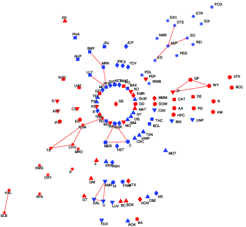
Figure 1: Sample graph of $N=116$ vertices and $n=20$ edges, corresponding to a connection probability $p=n/[N(N-1)/2]\approx 0.003$.

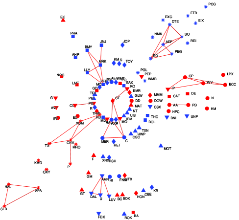
Figure 2: Sample graph for $n=40$ edges ($p\approx 0.006$).

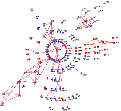
Figure 3: Sample graph for $n=80$ edges ($p\approx 0.012$).

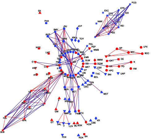
Figure 4: Sample graph for $n=160$ edges ($p\approx 0.024$).

Here we wish to focus more on the aspects of the growth and clustering for the same set of data, in particular for the asset graph. The most straight-forward way to see how the asset graph topology and clusters form is depicted as an example in Figures 1 to 4. Note that vertices are drawn using a variety of different markers, where the marker type and colour correspond to the company’s business sector as classified by Forbes forbes . For certain companies, such as those in the Energy Sector (marked by red asterisks) we would expect strong intra-business sector clustering, and for some, such as those in the Financial business sector (blue circles), we would expect strong inter-business sector clustering. There are also some stocks for which we would not expect graph clustering to correspond to the business sector labels (for a discussion on the correspondence between business sectors and asset tree clusters see long ).

Some observations and comments are in place.

(i) In Figure 1, after only $n=20$ edges have been added, already four cycles have formed. This makes it clear that asset tree and asset graph topologies start to diverge at an early stage, i.e., for small $n$.

(ii) In Figure 2, the additional 20 edges seem to reinforce the small clusters present in Figure 1. In general, it is interesting to note that the clusters created very early seem to become more and more strongly connected, and also grow by having new vertices attached to them as edges are added. It is not evident that the strongest connections (shortest edges) should define the clusters the way they do, as one could have a situation where a very strongly cliqued group of companies appears later on. However, moving from Figure 2 to 4, it is clear that this is what happens.

(iii) An asset tree defined on 116 vertices has 115 edges. In Figure 4, where the number of edges $n=160$ easily exceeds this, there are still several isolated vertices left. This turns out to be so even after 1000 edges have been added. The asset tree, however, would contain by definition those isolated vertices after the inclusion of $n=115$ edges. In this sense, although the asset tree can provide an overall taxonomy of the market, the connections it creates may be misinterpreted to be more meaningful than they are. As mentioned earlier and studied in intia , this due to the the minimum spanning tree criterion. Consequently, it is hardly surprising that an asset graph of the size of an asset tree is much more robust, since the weak connections contained in the tree are prone to breaking easily intia .

(iv) We can observe in Figure 4 that although some clusters are very heavily intra-connected, they are not yet inter-connected to other clusters. Two such examples are the energy cluster at the bottom left corner and the utilities cluster in the top right corner of Figure 4.

(v) In general, we see that there is good agreement between graph clusters and business sector definitions given by an outside institution.

(vi) Although the graph analysed here is just a sample, obtained by fixing the time, i.e., choosing a random value for the time superscript $t$, preliminary studies indicate that qualitatively similar clustering is observed throughout the time domain.

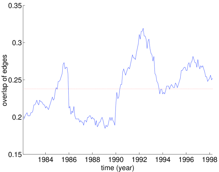
Figure 5: Overlap of edges in the asset graph $\mathbf{G}^{t}$ and asset tree $\mathbf{T}^{t}$ for $T=1000$ trading days as a function of time. The average value, roughly 24%, is indicated by the horizontal line.

As points (i) and (iii) above indicate, asset trees and asset graphs have clearly different topologies. Let us denote the asset graph more completely by its vertex and edge set as $\mathbf{G}^{t}=(V_{G},E_{G}^{t})$, and the asset tree similarly by $\mathbf{T}^{t}=(V_{T},E_{T}^{t})$. For statistically more reliable results, we have used a set of split-adjusted daily price data for $N=477$ NYSE traded stocks, time-wise extending from the beginning of 1980 to the end of 1999. This is the dataset we will use throughout the paper unless mentioned otherwise. We can learn about the overall topological differences between the asset graph and asset tree by studying the overlap of edges present in both as a function of time. The relative overlap is given by $\frac{1}{N-1}|E_{G}^{t}\cap E_{T}^{t}|$ where $\cap$ is the intersection operator and $|...|$ gives the number of elements in the set. As can be see from the plot in Figure 5, on average the asset graph and asset tree share about 24%, or roughly one quarter, of edges. This quantity is also fairly stable over time. Since the asset graph consists of the shortest possible edges and is optimal in this sense, whenever an edge in $E_{T}^{t}$ is not included in $E_{G}^{t}$, the sum of edges for the asset graph is increased above this optimum. Therefore, we can infer from Figure 5 that on average some 75% of the edges contained in the asset tree are not optimal in this sense. We drew a similar conclusion by comparing edge length distributions for the asset tree and asset graph in Figures 4 and 5 intia .

Motivated by observation (i) above, it is also of interest to study how this overlap of edges changes in the process of constructing asset graph and tree one edge at a time. In order to generate the minimum spanning tree, we use Kruskal’s algorithm. This consists of taking all of the distinct $N(N-1)/2$ distance elements from the distance matrix $\mathbf{D}^{t}$, and obtaining a sequence of edges $d_{1}^{t},d_{2}^{t},\ldots,d_{N(N-1)/2}^{t}$, where we have used a single index notation. The edges are then sorted in a nondecreasing order to get an ordered sequence $d_{(1)}^{t},d_{(2)}^{t},\ldots,d_{(N(N-1)/2)}^{t}$. We select the shortest unexamined edge for inclusion in the tree, with the condition that it does not form a cycle. If it does, we discard it, and move on to the next unexamined edge on the list. Apart from for the constraint on cycles, the algorithm is identical to the way asset graphs are generated. If we denote the size of graph in construction by $n$, where $n=1,2,\ldots,N-1$, then at least for small values of $n$ asset graphs and asset trees should contain the same set of edges, i.e., $E_{G}^{t}(n)=E_{T}^{t}(n)$ and, therefore, be identical in topology. It is expected that, starting from some value of $n=n_{c}$, the above equality no longer holds, and observation (i) above leads us to expect a small value for $n_{c}$. Once the equality breaks, the first cycle is formed and, consequently, for all $n\geq n_{c}$ the asset graph and tree differ topologically. This is demonstrated in Figure 6, where the relative overlap of edges, $\frac{1}{N-1}|E_{G}^{t}(n)\cap E_{T}^{t}(n)|$, has been plotted as a function of normalised number of edges, $\frac{n}{N-1}$, and the quantity has been averaged over time. The function decreases rapidly for small values of $\frac{n}{N-1}$, indicating that for the current set of data with $N=477$, only a few edges can be added before the first cycle is formed. As more and more edges are added, the plot converges to the 24% time average.

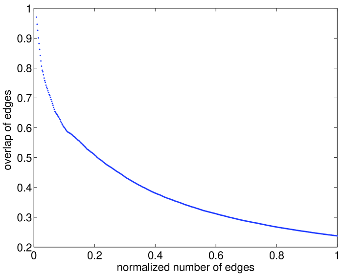
Figure 6: Overlap of edges $E_{G}^{t}(n)$ in the asset graph and $E_{T}^{t}(n)$ in the asset tree, where $n=1,2,\ldots,n$, as a function of normalised number of edges $\frac{n}{N-1}$, averaged over time.

IV Asset graph and random graph comparisons

We now leave asset trees behind and deal exclusively with asset graphs. We focus on our empirical sample graph $\mathbf{G}_{\text{emp}}$ evaluated from a distance matrix $\mathbf{D}^{t}$ for a randomly chosen time window location $t$. We then construct a random graph of the same size as the asset graph, and compare the results between the two. The fact the window is fairly wide at $T=1000$ means that the results are less sensitive to the time location $t$ of the window and, consequently, can be generalised to a greater extent than if a shorter window width was used. Time dependence of the quantities studied, as well as a more analytical approach in general, are postponed until a later exposition.

As should be clear from the earlier discussion, the asset tree approach as a simple, non-parametric classification scheme always produces a unique taxonomy. Because of the tree condition, the asset tree ignores some important correlations, and also fails to capture the strong networking present in the financial market. It is generally agreed that the correlation matrix contains both information and noise, and one is obviously interested in finding and studying the information rich part. In the extreme case of no information, one could find the minimum spanning tree for a completely random matrix of uncorrelated data. In this case one would also obtain a classification, but hardly a meaningful one. This indicates a possible drawback in the minimum spanning tree methodology.

Growth and clustering of asset graphs is an interesting problem in its own right, but it may also, as we believe, shed light on the information versus noise issue. We will now consider the size $n$ of the graph as a parameter and increase it, at least in theory, all the way up to the fully connected graph. If $d_{(n)}$ is the latest edge added, where $n=1,2,\ldots,N(N-1)/2$, we quantify the degree of graph completeness by $p=n/[N(N-1)/2]$, where $p\in[0,1]$. In practice, for our empirical data of $N=477$ stocks we do this for $p\in[0,0.25]$, corresponding to a maximum of 28,382 edges. In our experience this interval is sufficient, since most quantities beyond this become practically random anyway.

The random graph, or more specifically an Erdös-Rényi random graph, is denoted by $\mathbf{G}_{\text{ran}}$ and constructed as follows: Given $N$ labelled, isolated vertices, we consider all possible vertex pairs in turn and connect them with probability $p$. However, instead of generating the random graph explicitly from the definition, we obtain one by shuffling the elements in the distance matrix $\mathbf{D}^{t}$ and then add them, one edge at a time, to the graph. The graphs obtained at different stages of this process correspond to higher and higher connection probabilities $p$. This method enables us to compare graph construction for the empirical graph $\mathbf{G}(p)_{\text{emp}}$ and random graph $\mathbf{G}(p)_{\text{ran}}$ as a function of the connection probability $p$. Strictly speaking the results derived from the random-graph theory apply only in the limit when the number of nodes $N$ tends to infinity. Although the datasets we have studied have either $N=116$ or $N=477$, acknowledging the presence of finite size effects, one can consider the random graph as a benchmark against which deviations from random behaviour can be measured. As we will see, the financial network does not follow the predictions of the random graph theory and thus constitutes a complex network.

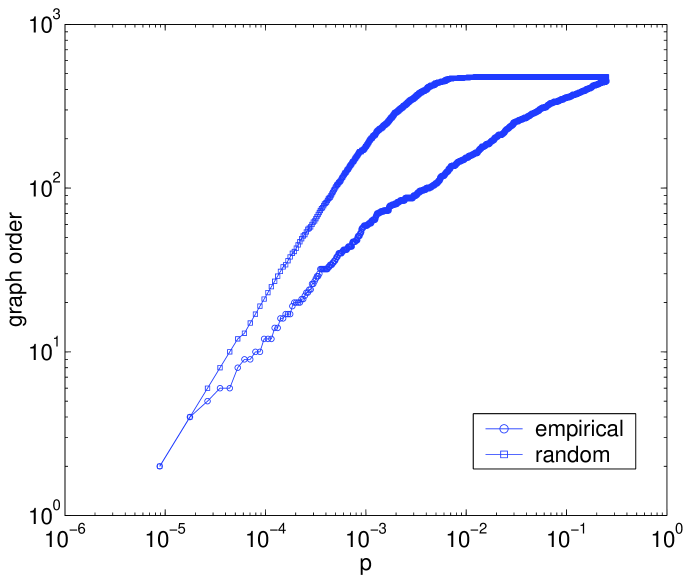
Figure 7: Spanned graph order for empirical and random data.

IV.1 Cluster growth and size

We start by studying what we call the spanned graph order. Whereas graph order indicates the number of vertices in the graph, we define spanned graph order as the number of vertices with vertex degrees greater than or equal to one, i.e., only those vertices are counted that have at least one edge connected to them. This distinction is needed because graph order itself is a constant for our graphs. Figure 7 plots spanned graph order for empirical and random data. We find that the random graph becomes fully connected very early on, i.e., its spanned graph order $\mathcal{S}(\mathbf{G_{\text{ran}}}(p^{\prime}))=N=477$ for $p^{\prime}\approx 0.012$, whereas for the empirical graph for the same value of $p$ we have $\mathcal{S}(\mathbf{G}_{\text{emp}}(p^{\prime}))=164$. In the empirical case, edges are used to create strong clusters and, therefore, the spanned graph order grows more slowly than for the random case, in which there is no systematic clustering present.

We can study some topological aspects of graph construction by considering four distinct types of growth that occur in the graphs. The division into these specific growth types is motivated by their intuitive appeal and relevance in this application context. These different types cause qualitatively different growth of graph clusters, and studying them can help us understand the differences we observe in greater detail. In the case of a financial network, edge clusters are more interesting than vertex clusters, because it is edges, i.e., correlations amongst stocks, that very naturally define clusters in the financial market, as Figures 1 to 4 show. A cluster, denoted by $\mathcal{C}_{i}=(V_{i},E_{i})$, is defined to be an isolated subgraph induced by a set of edges $E_{i}$, containing the vertices $V_{i}$. We also define cluster size of $\mathcal{C}_{i}$ simply as $|E_{i}|$. Similarly, cluster order for $\mathcal{C}_{i}$ is given by $|V_{i}|$. The four different growth types occurring upon the addition of a new edge $e_{ij}$, incident on vertices $v_{i}$ and $v_{j}$, are the following:

• Create a new cluster. This occurs when neither of the two vertices $v_{i}$ nor $v_{j}$, incident on the new edge $e_{ij}$, are part of an existing cluster. A new cluster is created, its spanned cluster order is two, and cluster size one.

• Add a node and an edge to an existing cluster. Adds vertex $v_{i}$ and the incident edge $e_{ij}$ to an existing cluster, when the other vertex $v_{j}$ already belongs to it. Spanned cluster order and cluster size are increased by one.

• Merge two clusters. Merge cluster $\mathcal{C}_{i}$ containing the vertex $v_{i}$ and cluster $\mathcal{C}_{j}$ containing the vertex $v_{j}$ by adding the incident edge $e{{}_{ij}}$ between them. If $|E_{i}|\geq|E_{j}|$, the cluster $\mathcal{C}_{i}$ survives and its new order is $|V_{i}|+|V_{j}|$ and new size $|E_{i}|+|E_{j}|+1$. Cluster $\mathcal{C}_{j}$ disappears as we have $E_{j}=\emptyset$ and $V_{j}=\emptyset$. Intuitively speaking, the larger cluster eats the smaller one.

• Add a cycle to an existing cluster. Add an edge to an existing cluster, thus creating a cycle and reinforcing the clustering. Spanned graph order is increased by one.

The cumulative occurrence of each growth type is plotted as a function of $p$ for random data in Figure 8 and for empirical data in Figure 9. Some observations. (i) The growth of the random graph starts linearly with type I and continues like that practically for two decades, as new clusters of one edge and two vertices are created. As a result, the number of vertices grows by two on each step, contributing to the rapid increase in spanned graph order for the random graph in Figure 7. Type I growth is clearly less dominant for the empirical graph, for which growth of other types starts earlier. (ii) In regard to clustering, type IV growth is most relevant and is observed roughly 1.5 decades earlier for the empirical data than for the random data. This finding is corroborated by Figures 1 to 4 and the related discussion. (iii) We observe that the number of types I and III growth almost converge as $p\to 1$. The convergence is to be expected since in moving towards a fully connected graph, all the separate clusters that have been formed will be merged at some point. Thus in the limit the number of mergers needs to equal the number of components to be merged minus one, since one cluster, the fully connected graph, remains. The convergence seems to take place an estimated 1.5 decades later for the empirical graph than for the random graph, indicating that the clusters observed for the empirical data remain separate or disconnected from the rest until much later.

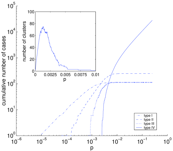
Figure 8: Growth types for the random graph. Inset: number of clusters for the random graph.

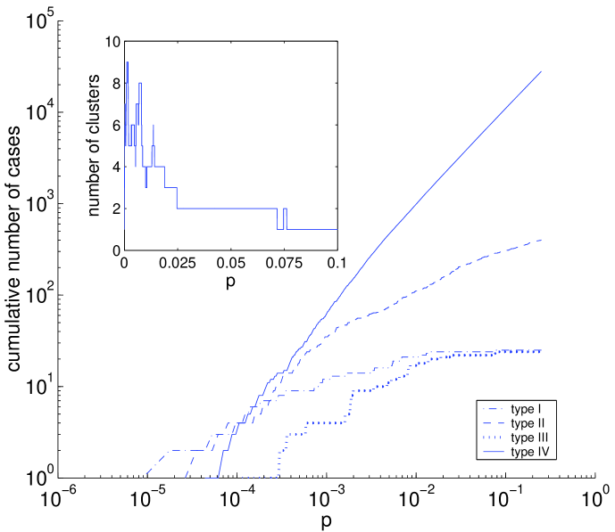
Figure 9: Growth types for the empirical graph. Inset: Number of clusters for the empirical graph.

Let us now study the number of clusters formed as a function of $p$. Of the four growth types analysed above, only type I and type III affect the number of clusters in the system, by either increasing or decreasing it by one, respectively. Therefore, the number of clusters for a given value of $p$ is given by the difference between type I and type III curves in Figures 8 and 9. This is more clearly shown on linear scales in the insets of the same figures (please note that the scales in the insets are different). The maximum number of clusters for the sample random graph is 75, occurring at $p\approx 0.0013$, whereas for the empirical graph it is 9, occurring at $p\approx 0.0011$. The high spanned graph order for the random graph due to type I growth, and relatively low mean clustering coefficient as compared to the asset graph (as seen later), leads to a large number of clusters that are relatively early combined to form one giant cluster. In contrast, the empirical graph has a much more slowly increasing spanned graph order, fewer clusters, and exhibits predominantly type IV growth to enhance the existing clusters (high mean clustering). Consequently, the maximum number of clusters is left small. It is interesting to note that in this case the maxima, although very different in value, happen for roughly the same value of $p$. Further studies are required to explain whether this is by chance or a systematic finding.

Let us now turn to cluster size distributions presented in Figures 10 and 11. For the random graph, the large number of clusters seem to disappear suddenly when the clusters are merged together, as the sudden jump in type III growth in Figure 8 indicates. This type of sudden transition is not present for the empirical graph, further supporting the conjecture that the behaviour of the asset graph is markedly different from the random graph.

The results we have obtained for the random graph are well explained by some basic random graph theory, from which we wish to review very briefly some important elementary findings barabasi . This will help not only to explain the random results, but may also help to understand why the empirical graph behaves so differently. The most central goal of random-graph theory is to determine at what connection probability $p$ a particular property of a graph will most likely arise. In most general terms, we can ask whether there is a critical probability that marks the appearance of arbitrary subgraphs and, as its important special cases, trees and cycles of a given order. The problem was solved by Bollobás bollobas . Consider a random graph with $N$ vertices connected by $n$ edges and assume that the connection probability $p(N)\propto N^{z}$, where the parameter $z\in(-\infty,0]$. For a random graph, the average degree is given by

$$\langle k\rangle=2n/N=p(N-1)\approx pN,$$

and this quantity has a system size independent critical value. When $z<-1$ such that the average degree of the graph $\langle k\rangle=pN\to 0$ as $N\to\infty$, the graph consists of disjoint trees. The appearance of these small trees is tied to some threshold values of $z$ such that below that value almost no graph has the given property, whereas for values above it almost every graph has the property. What is remarkable from our perspective is that for $z<-1$ there are no cycles present, but when $z=-1$, corresponding to $\langle k\rangle=$ constant, trees and cycles of all orders appear. We can find out about the size and structure of clusters for this particular case when $p\propto N^{-1}$. When $0<\langle k\rangle<1$, although there are cycles present, almost all nodes belong to trees, and the size of the largest tree is proportional to $\ln N$. The mean number of clusters is of order $N-n$, so in this range of $\langle k\rangle$ the number of clusters decreases by 1 as $n$ increases by 1, i.e., when a new edge is introduced in the graph. If $\langle k\rangle$ is increased to the threshold $\langle k\rangle_{c}=1$, corresponding to a critical probability $p_{c}\approx 1/N$, the topology of the graph changes suddenly. The small clusters are merged together to form a single giant cluster, or a giant component, and it has a fairly complex structure. Other clusters are small, and most of them are trees. As $\langle k\rangle$ is increased further, the small clusters are attached to the giant cluster. Therefore, for values below $p_{c}$ the graph is made up of isolated clusters, but for values above $p_{c}$ the giant cluster spans the graph. Given these theoretical considerations, the fact that cycles are found in the graphs in Figures 1 to 4, even for $p\approx 0.003$, underlines the highly correlated “non-random” nature of the financial network. Last, as a point concerning terminology, it should be mentioned that the emergence of the giant cluster is the same phenomenon as a percolation transition in infinite-dimensional (mean field) percolation. The difference in the behaviour around the emergence of the giant component between the random and empirical graph indicates that the transition in the latter is also of different nature.

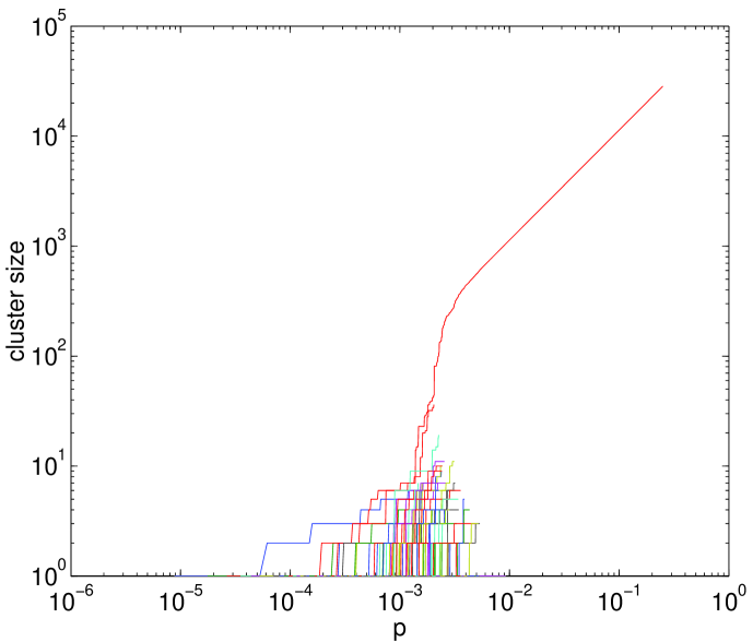
Figure 10: Cluster size for the random graph. Different curves correspond to different clusters. Since several clusters of size one overlap one another in this figure rendering them indistinguishable, one cannot count the total number of clusters from this plot.

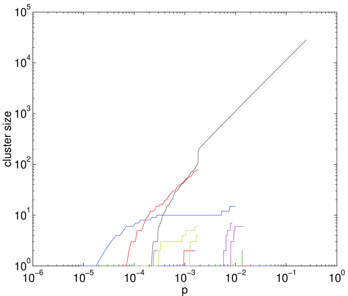
Figure 11: Cluster size for the empirical graph. See comment in Figure 10.

IV.2 Clustering coefficients and information

Finally, we will study the clustering coefficients for our smaller set of 116 S&P500 stocks. Clustering coefficient of vertex $i$ is defined as

$$C_{i}=\frac{2\Delta_{i}}{k_{i}(k_{i}-1)},$$

where $k_{i}$ is the number of incident edges of vertex $v_{i}$ (vertex degree), and $\Delta_{i}$ the number of edges that exist between the $k_{i}$ neighbours of vertex $v_{i}$. The normalisation in the definition is due to the fact that at most there can be $k_{i}(k_{i}-1)/2$ edges between the $k_{i}$ vertices, which would happen if they formed a fully connected subgraph. Thus the coefficient is normalised on the interval $[0,1]$. The value of clustering coefficient for each vertex $v_{1},v_{2},\ldots,v_{116}$ is plotted in Figure 12 for both the random graph and empirical graph, where the vertex index is given on the horizontal axes, the vertical axes give the value of $p$, and the shades corresponds to the value of the clustering coefficient. The two plots are strikingly different. For the random graph, overall there is a very smooth, rainbow-like transition from zero to unity. In addition, all vertices behave in a fairly homogeneous manner. For the empirical graph the transition towards unity is much faster and there is much greater heterogeneity present. Further, there are some very high clustering coefficient values observed for some vertices at low values of $p$.

Since much of our attention has focused on asset graph clusters, we calculated clustering coefficients of the sample graph for each cluster when $p\in[0,1]$. These are simply averages of the clustering coefficients $C_{i}$ of individual vertices belonging to a given cluster $\mathcal{C}_{i}$, i.e.,

$$C_{\mathcal{C}_{i}}=\frac{1}{|V_{i}|}\sum_{C_{i}\in\mathcal{C}_{i}}C_{i}.$$

In Figure 13 we show results for selected six clusters, namely, Transportation, Energy, Utilities, Basic Materials 1, Utilities / Healthcare, and Basic Materials 2. For values of $p\geq 0.05$ all other clusters coalesce into the Utilities / Healthcare cluster, which behaves very similarly to the mean clustering coefficient discussed shortly. The small deviations result from the fact that there are some isolated vertices which are not included in the coalesced cluster but are counted in the mean clustering coefficient. For purposes of visualisation only clusters with six or more edges are included in Figure 13, as for smaller clusters the clustering coefficient fluctuates wildly and makes the plot messy. Further, only those clusters with reasonably long life time in terms of $p$ are included.

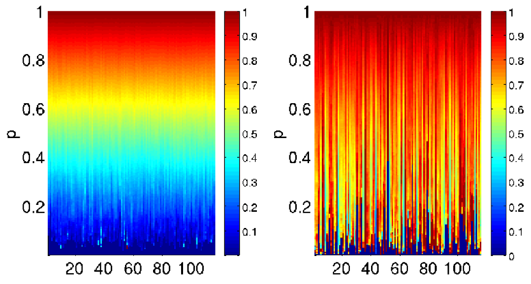
Figure 12: Clustering coefficient as a function of vertex index (horizontal axis) and $p$ (vertical axis). Left: random graph, right: empirical graph.

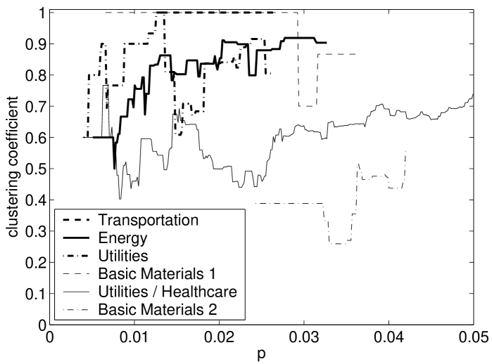
Figure 13: Clustering coefficients for selected clusters as a function of $p$.

In most cases each cluster consists of stocks that belong to different business sectors. The clusters are named after the dominating business sector, i.e., the business sector shared by a majority of the vertices in the cluster. Apart from one exception, a single business sector dominates for each value of $p$, indicating strong correspondence between cluster and business sector groups. The only exception is the largest cluster, i.e., Utilities / Healthcare, which was dominated by either Utilities or Healthcare stocks, depending on the value of $p$.

The four most highly connected clusters are Transportation, Basic Materials 1, Utilities, and Energy. The cluster-wise calculated clustering coefficients are more meaningful when examined in conjunction with Figures 1 to 4. One should also bear in mind that cluster sizes and cluster orders for the four clusters are different, and this needs to be taken into account when studying clustering coefficients. Although cluster sizes for these clusters are not reported in this paper for the particular set of data, it is clear that for larger clusters there is more jitter in the curves of Figure 13. The Transportation cluster consists, for the most part, of stocks AMR, DAL, U and LUV and is fully connected, as there is an edge between DAL and LUV, although poorly visible. Basic Materials 1 cluster consists of stocks IP, GP, WY and BCC, and they are also fully connected for $p\in[0.005,0.03]$, but clustering falls as new vertex is added to the cluster. The most striking examples, however, are Utilities and Energy clusters, both of which encompass several vertices. As Figure 4 shows, they are very strongly connected. Quite remarkably, both clusters are also very homogeneous in terms of their business sector makeup. These findings indicate that in the financial network there are clusters that are relatively separate from others, and yet their internal connectivity is high.

By averaging the clustering coefficients $C_{i}$ over all vertices $i$ one obtains the mean clustering coefficient $C_{\text{ran}}$ and $C_{\text{emp}}$, both plotted in Figure 14. From this plot the difference in the rate of change of the clustering coefficient for the random and empirical case is very obvious. For the random graph the mean clustering coefficient is zero up to and including $p^{\prime}=125/6670\approx 0.02$, whereas for the empirical graph for the same $p=p^{\prime}$ the mean clustering coefficient is 0.33. For the random graph, the zero value and low values at the beginning in general are again explained by type I growth leading to duple clusters (one edge, two vertices), for which the clustering coefficient is zero. For the empirical graph the early type IV growth creates several cycles of order three as can be seen, for example, in Figure 1. For these cycles the clustering coefficient is unity, and this contributes to the mean clustering coefficient. To visualise the empirical graph with 125 edges, one can mentally interpolate between Figures 3 and 4 to convince himself or herself of the high mean clustering coefficient value. Please note that the clustering coefficient results can directly be compared only with Figures 1 to 4, since for other random and empirical graph plots a different dataset was used.

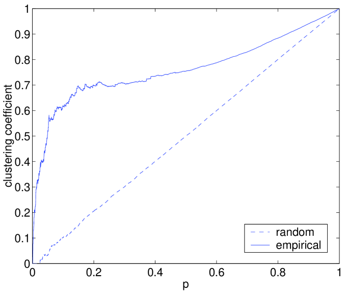
Figure 14: Mean clustering coefficients for the random and empirical graph as a function of $p$.

The mean clustering coefficient for the random graph, for all practical purposes, is linear with a slope of unity (except for the slight fluctuation for small $p$). This result is compatible with random graph theory, since for a random network, the probability of its two nearest neighbours being connected is the same as that for any two randomly picked vertices being connected. Therefore, the mean clustering coefficient for a random graph is

$$C_{\text{ran}}=p=\frac{\langle k\rangle}{N}.$$

We conjecture that comparing the mean clustering coefficient of an empirical asset graph against a random graph can be used to estimate the information content of the edges in the graph and, consequently, the information content of the corresponding correlation coefficients in the related correlation matrix. For a rough analysis of results we divide the empirical curve in Figure 14, based on its behaviour, into three sections along the horizontal axis. The first section of rapid growth covers the first 10% of edges ($p\in[0,0.1]$), during which the mean clustering coefficient increases very rapidly and, in particular, much faster than for the random graph. We interpret this significant deviation from the random case to imply that the first 10% of the edges add substantial information to the system. During the first part of the second section for roughly $p\in[0.1,0.2]$, the rate of change starts to slow down and reaches a sort of a plateau or saturation during the second part of this section for $p\in[0.2,0.3]$. We consider these findings to indicate that the edges added in this section for $p\in[0.1,0.3]$ are less informative. For the last section, from $p=0.3$ onwards, we believe the remaining 70% to be relatively poor in information content, possibly just noise. Although the curve becomes steeper as $p\to 1$, we do not consider this to reflect genuine information but to result from the boundary conditions of the problem, since for $p=1$ the mean clustering coefficient must be equal to unity.

We believe that the method of comparing empirical graph properties to random graph theory predictions can be used to address the information versus noise issue of the underlying correlation matrix. In spirit this is a similar argument to using random matrix theory to study the information content of empirical correlation matrices by comparing their properties, mainly eigenvalue spectra. In Lal , there was remarkable agreement between the theoretical prediction and empirical data concerning both the density of eigenvalues and the structure of eigenvectors for the correlation matrix. For their set of $N=406$ assets of the S&P 500 for $T=1309$ days, Laloux et al found 94% of the total number of eigenvalues to fall within the region predicted by the theory, leaving only 6% of the eigenvectors to appear to carry some information. This finding is compatible with the above discussion. We plan to repeat this analysis for a larger set of data in the near future and carry it out dynamically.

V Summary and Conclusion

In this paper we have recapitulated the methodology for constructing asset graphs and asset trees. Due to the tree condition, the asset tree fails to capture the strong clustering in the financial market, but this is clearly present in the asset graph. We have found the clusters in the asset graph to appear very early, i.e., for low connection probabilities, after which asset graph and asset tree topologies begin to differ. The two methodologies result in an approximate 25% overlap of edges over time, and the remaining 75% cause them to exhibit qualitatively very different behaviour. We have studied the asset graph further and compared the results to a random graph of the same size as a function of connection probability. We have divided the growth processes into four distinct growth types, and have found type I growth to be responsible for the fast growth in spanned graph order for the random graph. A study of growth types has also revealed how type IV growth, responsible for creating cycles in the graph, sets in much earlier for the asset graph, and thus reflects the networking present in the market. We have also found the number of clusters in the random graph to be one order of magnitude higher than for the asset graph. At a critical threshold, the random graph undergoes a radical change in topology, when the small clusters merge to form a single giant cluster. This phenomenon, equivalent to a percolation transition, is not observed for the asset graph. Finally, we have studied clustering coefficients and mean clustering coefficients, and found them to behave very differently for the asset and random graph. We have conjectured that this difference may be suitable for studying what fraction of edges in the graph, or correlation coefficients in the related correlation matrix, is information and what is noise. Based on this approach, only some 10% of the edges appear to carry genuine information. The results presented in this paper concerning asset and random graph comparisons have been carried out for a randomly selected but representative time window and a more rigorous study should be made to include the possible effects of time dependence.

Acknowledgements

We are thankful to A. Chakraborti who participated in earlier stages of this work. J.-P. O. is grateful to the Graduate School in Computational Methods of Information Technology (ComMIT), Finland. This research was partially supported by the Academy of Finland, Research Centre for Computational Science and Engineering, project no. 44897 (Finnish Centre of Excellence Programme 2000-2005).

References

- (1) W. B. Arthur, S. N. Durlauf and D. A. Lane (eds.), The economy as an evolving complex system II, Addison-Wesley, Reading, Massachusetts (1997).
- (2) H. M. Markowitz, Journal of Finance 7, 77 (1952).
- (3) R. Albert and A.-L. Barabási, Rev. Mod. Phys. 74, 47 (2002), S.N. Dorogovtsev and J.F.F. Mendes: Evolution of Networks: From Biological Nets to the Internet and WWW (Oxford UP, 2003).
- (4) G. Caldarelli, S. Battiston, D. Garlaschelli and M. Catanzaro, In "Complex Networks", Springer, 2004, Eds. E.Ben-Naim, H. Frauenfelder and Z. Toroczkai.
- (5) J.-P. Onnela, A. Chakraborti, K. Kaski, J. Kertesz, and A. Kanto, Phys. Scr. T 106, 48 (2003).
- (6) R. N. Mantegna, Eur. Phys. J. B 11, 193 (1999).
- (7) L. Kullmann, J. Kertész and R. Mantegna, Physica A 287, 412 (2000)
- (8) J.-P. Onnela, A. Chakraborti, K. Kaski and J. Kertész, Eur. Phys. J. B 30, 285 (2002).
- (9) J.-P. Onnela, A. Chakraborti, K. Kaski, J. Kertész, and A. Kanto, Phys. Rev. E 68, 056110 (2003).
- (10) J.-P. Onnela, A. Chakraborti, K. Kaski and J. Kertész, Physica A 324, 247 (2003).
- (11) G. Bonanno, F. Lillo and R. N. Mantegna, Quantitative Finance 1, 96-104 (2001).
- (12) G. Bonanno, N. Vandewalle and R. N. Mantegna, Phys. Rev. E 62, R7615 (2000).
- (13) L. Kullmann, J. Kertész and K. Kaski, Phys. Rev. E 66, 026125 (2002).
- (14) M. Mehta, Random Matrices, Academic Press, New York (1995).
- (15) L. Laloux et al., Phys. Rev. Lett. 83, 1467 (1999).
- (16) V. Plerou et al., Phys. Rev. Lett. 83, 1471 (1999).
- (17) S. Pafka and I. Kondor, Physica A 319, 487 (2003).
- (18) I.T. Joliffe: Principal Component Analysis (2002, Heidelberg, Springer), R. Brummelhuis, A. Cordoba, M. Quintanilla and L. Seco, Mathematical Finance 12, 23 (2002)
- (19) A. Hyvärinen, Neural Computing Surveys, 2, 94 (1999), A.D. Back and A. Weigend, International Journal of Neural System, 8, 473-484 (1997).
- (20) B. Bollobás, Random Graphs (2nd ed.), Cambridge University Press (2001).
- (21) Forbes at http://www.forbes.com/, referenced in March-April, 2002.