On ground states of interacting Composite Fermions with spin at half filling.

Abstract

The effects of interactions in a 2D electron system in a strong magnetic field of two degenerate Landau levels with opposite spins and at filling factors $1/2$ are studied. Using the Chern-Simons gauge transformation, the system is mapped to Composite Fermions. The fluctuations of the gauge field induce an effective interaction between the Composite Fermions which can be attractive in both the particle-particle and in the particle-hole channel. As a consequence, a spin-singlet (s-wave) ground state of Composite Fermions can exist with a finite pair-breaking energy gap for particle-particle or particle-hole pairs. The competition between these two possible ground states is discussed. For long-range Coulomb interaction the particle-particle state is favored if the interaction strength is small. With increasing interaction strength there is a crossover towards the particle-hole state. If the interaction is short range, only the particle-particle state is possible.

I Introduction

The Composite Fermion (CF) model for the fractional quantum Hall effect (FQHE) has been very successful in describing in a simple and intuitive way the basic filling factors at which this complex collective phenomenon occurs. Jain89 One route to CFs is the Chern-Simons (CS) gauge transformation which maps a system of interacting electrons in a Landau level (LL) at an even-denominator fractional filling into a weakly interacting Fermi liquid of CFs.SternHalp95 ; LF91 ; HLR93 This is achieved by formally attaching an even number of flux quanta to each electron. On the average, the CFs do not see the external magnetic field but a smaller effective one, which vanishes in mean field approximation at the even-denominator fractional filling considered. The Coulomb interaction between the electrons is in this model incorporated into a finite effective mass.Books The incompressible states responsible for the FQHE of the electrons can then be described in terms of integer quantum Hall states of the CFs. Experimental support for the model comes from measurements near filling factor one half.willett Theoretical expectations concerning the properties of the CFs HLR93 have been confirmed by surface-acoustic wavesaw and transport experiments in periodically modulated structuresanti and from cyclotron resonance.k02

The results obtained until now suggest that constructing compound quasi particle states made of charges and fluxes in such a way that the repulsive interaction is minimized is a very efficient way of dealing with strongly interacting many particle systems. Better understanding of such states may be of great importance beyond explaining the fractional quantum Hall effect. High-$T_{\rm c}$-superconductivitybm86 , the unique properties of heavy fermion systemsgs91 , and the recently discovered metal-insulator transition in low density two dimensional electron systemsks03 can be suspected to be candidate systems where the concept of compound charge-flux quasi particles may eventually turn out to be crucial for understanding the underlying correlations. Thus, one is led to conclude that studying the physics of charge-flux states is an important subject of research in its own right.

At high magnetic field one often can safely assume that the spins are frozen such that the quantum Hall states are spin polarized. However, due to the small value of the electron $g$-factor in GaAs ($\approx-0.4$), this assumption is not always valid, especially for the smaller magnetic field strengths sufficient to enter the region of the FQHE in the lowest Landau level for samples with low electron density. It has been experimentally established that, depending on the filling factor, FQHE states may be unpolarizedcetal89 ; eetal89 ; eetal90 ; eetal92 ($\nu=4/3,8/5,10/7,2/3$) or partially polarized ($\nu=3/5,7/5$).cetal89 ; eetal92 There are also crossovers between different polarizations when changing the Zeeman splitting by tilting the magnetic field, or when reducing the electron density. The spin polarization of several FQHE states has been optically determined Kukushkin at fixed filling factors as a function of the ratio between Zeeman and Coulomb energies,

$$\xi=\frac{E_{\rm Z}}{E_{\rm C}}\,$$ (1)

where

$$E_{\rm C}=\frac{e^{2}}{\epsilon l_{B}}$$ (2)

and $\epsilon$ and $l_{B}=\sqrt{\hbar c/eB}$ are respectively the dielectric constant and the magnetic length.

Crossovers between differently spin polarized ground states for the same FQHE filling factor have been detected. The spin polarization remains constant within large intervals of $\xi$. Near certain critical values $\xi_{\rm cr}$, the system undergoes a transition between differently spin-polarized CF states. A simple model of non-interacting CFs with spin with an effective mass that scales as the Coulomb interaction, i.e. $m^{*}\propto\sqrt{B}$, can explain the experimental data. The broad plateaus of constant spin polarization are due to the occupation of a fixed number of spin split LL of the CFs (CFLL). The crossovers occur when intersections of CFLLs with opposite spins coincide with the chemical potential.annalen

The optically determined spin polarizations, when extrapolated to zero temperature, show additional plateaus for flux densities near the centers of the crossovers. The corresponding polarizations are almost exactly intermediate between those in the neighboring broad plateaus within the experimental uncertainties. This indicates additional physics beyond the non-interacting CF model. The intermediate plateaus can be interpreted as the signature of new collective states since one can expect that if two CFLLs are degenerate, interactions between CFs become very important and cannot be treated perturbatively. In these optical experiments, the CFLL have been tuned to degeneracy by using the magnetic field dependence of the effective mass of the CFs. Intermediate plateaus have also been observed with NMR where $\xi$ was changed by tilting the magnetic field.fetal01

Recent experimental studies of the FQHE in GaAs/AlGaAs samples of densities $\approx 10^{11}$ cm^-2 revealed strong FQHE-structures at filling factors $\nu=4/11$ and $5/13$ and weaker structures at $6/17$, $4/13$, $5/17$ and $7/11$.petal03 The feature at $4/11$ is independent of an in-plane component of the magnetic field and is expected to be spin polarized. These new FQHE states cannot be explained within standard sequences of IQHE of CFs. It seems that rather they are signature of a FQHE of CFs. This could imply that interaction between CFs can be expected to be strong.

One may summarize the above observations by noting that on the one hand spin is an important ingredient of the physics of composite charge-flux quasi particles that must not be neglected, and on the other hand that the interactions between the quasi particles may lead to qualitatively new collective quantum states. Better understanding of the latter, especially in the presence of spin, seems imperative not only for explaining the rich phenomena of the physics of the FQHEm03 but could also lead eventually to new insights into the physics of low dimensional many body systems.

Without using the CF model, several possibilities for the states that could form under the above conditions have been discussed.Murthy00 ; a01 However, in order to systematically understand interaction-induced and spin polarization properties of the FQHE states, the CF model can be expected to be useful.pj98 The first step is to generalize the CS-transformation to include the electron spin. With this supplementary degree of freedom, useful analogies can be drawn with bilayer systems of spinless fermions, where the electrons carry a layer - instead of a spin - index. This generalization to 2-component systems of CFs with index $s=\uparrow,\downarrow$ (or $1,2$) can be achieved with models in which a doublet of Chern-Simons gauge fields is introducedlopfrad01 ; its Lagrangian contains a $2\times 2$ matrix $\Theta_{ss^{\prime}}$

$$\Theta=\left(\begin{array}[]{cc}\theta_{1}&\theta_{2}\\ \theta_{2}&\theta_{1}\end{array}\right)\,,$$ (5)

which controls the attachment of flux quanta to the two species of fermions [see (13) below for details]. In the spin case, with such an approach many of the FQHE wave functions proposed hitherto for FQHE systems, with their spin polarizations, have been reproduced.mr96

In the bilayer system at total filling factor 1, and such that in each layer $\nu=1/2$, it has been arguedketal01 ; m02 that for small layer distance a spin-polarized p-symmetric pair state can be formed that is equivalent to the so-called (1,1,1)-state proposed earlier.h83 This state consists of pairs of interlayer (or mutual v02 ; ye03 ) CFs: $\Theta$ is chosen in such a way ($\theta_{1}=0,\theta_{2}=1/2$) that an electron in one layer is attached to two flux quanta in the other layer and vice versa. In this language, the CFs are attractively interacting interlayer dipolar objects, due to the fluxes being equivalent to ”holes” in the electron system; this is believed to be a possible mechanism for the interlayer phase coherence recently found in experiments in this regime.sp00 In general, different choices of $\Theta$ that preserve the fermionic statistics of the original particles can be exploited to describe the system when the layer distance is varied: a diagonal attachment of 2 flux quanta ($\theta_{1}=1/2,\theta_{2}=0$) is thought to describe correctly the intermediate- and large- distance regime of bilayers.ketal01

In the single layer with spin, generalized CFs have been introduced by a non-unitary Rajaraman-Sondhiraj96 instead of the CS-transformation.m00 The effective interaction between them contains the repulsive long-range Coulomb part, a contribution due to the gauge field fluctuations and a non-Hermitian term that destabilizes the CF states. Neglecting the non-Hermitian term, it was found that due to the symmetry of the gauge field term in the electron-electron interaction, which enters here in first order, s-wave pairing is not possible in static mean field approximation. By estimating the condensation energies it was found that if a pair state at total filling factor 1/2 was realized it would be a spin polarized p-wave state. Due the static mean field character of the approximation used, off-diagonal terms in the matrix $\Theta$ are needed in this approach to couple the two spins.

In the present paper, we reconsider the effective interaction between CFs with spin. Especially, we concentrate on the competition between the formation of particle-particle (p-p) and particle-hole (p-h) pairs in the s-wave channel. We consider a spin degenerate lowest Landau level at filling factor unity and assume that $N$ electrons are distributed among the available states in such a way that exactly half of them have spin $\uparrow$ and the other half have spin $\downarrow$. This is equivalent to two degenerate half-filled LL with opposite spins such that for each the CS transformation can be applied in order to obtain CFs. We assume that only the diagonal parts of the coupling matrix are non-zero,

$$\Theta=\left(\begin{array}[]{cc}1/2&0\\ 0&1/2\end{array}\right)\,.$$ (8)

The two subsystems are then transformed to two Fermi seas with $\uparrow$ and $\downarrow$ coupled by the effective CF interaction. We show that under this condition, the CS gauge field fluctuations can mediate an attractive interaction between CF-particles. In order to obtain this interaction in lowest order, we need to take into account an RPA-like renormalization of the gauge field fluctuations by the coupling to the CFs. The attractive interaction can result in a spin-singlet s-wave bound state of pairs of CF particles.metal02 ; pss ; varenna Alternatively, CF-holes and CF-particles may be bound together, thus forming an excitonic spin-singlet state. We consider the competition between the latter exciton-like and the former Cooper pair-like pairings in the CF system. We determine the corresponding pair breaking energy gaps, and the ground state energies. We discuss the stability of the different phases. For Coulomb interaction between the electrons we find that when the interaction strength measured by the Coulomb energy $E_{\rm C}$ is small the Cooper pair-like phase is more stable. When $E_{\rm C}$ is large compared with the chemical potential, the exciton-like phase is more stable. For short range interaction, the Cooper pair-like phase has always the lowest energy. We conjecture that the paired singlet phases are very likely to approximate the ground state of the interacting electron system even if the lowest LL is only close to spin degeneracy. Then, at zero temperature, the energetically lower LL with, say, spin $\uparrow$ will be occupied. However, if the gain in the ground state energy by forming a pair exceeds the cost in energy for occupying a state in the LL with spin $\downarrow$, pairs will be formed and the system will condense into the spin-singlet ground state.

The above model does not exactly match the situations in the aforementioned optical experiments where CFLLs with opposite spins corresponding to different Landau quantum numbers coincide. However, the second generation CFs can provide the scheme for understanding the additional plateaus at intermediate spin polarizations.metal02 ; annalen In any case, we feel that the effect of the residual interactions between CFs and whether or not they can give rise to new features is an interesting problem in its own right and deserves intense studies.

The paper is organized as follows. In section II the methods used to determine the effective interaction and the ground state are described. In section III, the particle-particle (p-p) and the particle-hole (p-h) ground-state energies are calculated for Coulomb interaction. In section IV the results are provided for short-range interaction. The phase-diagrams for the ground states are derived. Discussion of the results and final remarks will conclude the paper.

II Effective interaction and ground state properties

We consider two half-filled LL with opposite spins at the same energy. The CS-transformation is used to construct two 2D Fermi seas of CFs with spin and a Fermi wave number $k_{\rm F}=\sqrt{2\pi\rho}$ ($\rho$ total average electron number density).HLR93 An effective interaction between the CFs can be obtained from the Lagrangian density of the two coupled Fermi systems of charge $e$ (units $\hbar=c=1$),

$${\cal L}({\bf r},t)={\cal L}_{\rm F}({\bf r},t)+{\cal L}_{{\rm CS}}({\bf r},t)+{\cal L}_{{\rm I}}({\bf r},t)$$ (9)

with the kinetic energy of the Fermions

$${\cal L}_{\rm F}({\bf r},t) = \sum_{s=\uparrow,\downarrow}\psi^{\dagger}_{s}({\bf r},t)\Big{\{}i\partial_{t}+\mu+ea_{0}^{s}({\bf r},t)\Big{.}$$

$$-\frac{1}{2m}\Big{[}i\nabla + e\Big{(}{\bf A}({\bf r})-{\bf a}^{s}({\bf r},t)\Big{)}\Big{]}^{2}\Big{\}}\psi_{s}({\bf r},t)$$ (10)

($m$ effective mass, $\mu$ chemical potential), the CS term

$${\cal L}_{{\rm CS}}({\bf r},t)=-\frac{e}{\phi_{0}}\sum_{s,s^{\prime}}\Theta_{ss^{\prime}}\,a_{0}^{s}({\bf r},t)\,{\bf\hat{z}}\cdot\nabla\times{\bf a}^{s^{\prime}}({\bf r},t)$$ (11)

($\phi_{0}=hc/e$ flux quantum, ${\bf\hat{z}}$ unit vector perpendicular to the 2D plane), and the contribution of the electron-electron interaction

$${\cal L}_{{\rm I}}({\bf r},t)=-{\frac{1}{2}}\sum_{s,s^{\prime}}\int d^{2}r^{\prime}\rho_{s}({\bf r},t)V({\bf r}-{\bf r}^{\prime})\rho_{s^{\prime}}({\bf r}^{\prime},t).$$ (12)

Here, $\rho_{s}({\bf r},t)\equiv\psi^{\dagger}_{s}({\bf r},t)\psi_{s}({\bf r},t)$ is the density of the Fermions with spin orientation $s$, ${\bf A}$ the vector potential of the external magnetic field, $(a_{0},{\bf a})$ the CS gauge field, and $V({\bf r})$ the electron-electron interaction potential. The attachment of flux quanta $\phi_{0}$ to each Fermion is achieved by the Chern-Simons term ${\cal L}_{{\rm CS}}$ as can be seen by minimizing the action with respect to the $a_{0}^{s}$-gauge field. This gives the constraint

$$\sum_{s^{\prime}}\Theta_{ss^{\prime}}{\bf\hat{z}}\cdot\nabla\times{\bf a}^{s^{\prime}}({\bf r},t)=\phi_{0}\rho_{s}({\bf r},t).$$ (13)

The flux attachment for the two species of Fermions is in this paper performed independently. This corresponds to assuming the coupling matrix to be diagonal:

$$\Theta=\left(\begin{array}[]{cc}\theta_{1}&0\\ 0&\theta_{1}\end{array}\right).$$ (16)

We assume $\theta_{1}=1/2$, such that the mean fictitious magnetic field cancels the external one at half filling, $\nu\equiv\rho\phi_{0}/2B=1/2$. We use the transverse gauge, $\nabla\cdot{\bf a}^{s}=0$. The Bosonic variables associated with the gauge field fluctuations are the transverse components of their Fourier transforms, $a_{1}^{s}({\bf q},\omega)\equiv{\bf\hat{z}}\cdot\hat{\bf q}\times[{\bf a}^{s}({\bf q},\omega)-\langle{\bf a}^{s}({\bf q},\omega)\rangle]$. From the terms linear in the charge $e$ and the momentum $-i\nabla$, one can extract the form of the vertices connecting two Fermions with one gauge field fluctuation operator $a_{\mu}^{s}({\bf q},\omega)$ ($\mu=0,1$)

$$v^{s}_{\mu}({\bf k},{\bf q})=\biggl{(}\begin{array}[]{c}e\\ \frac{e}{m}\,{\bf\hat{z}}\cdot\frac{{\bf k}\times{\bf q}}{|{\bf q}|}\end{array}\biggr{)}.$$ (17)

In addition, there is a Fermion-gauge field coupling term quadratic in the fluctuations $w_{\mu\nu}^{s}=-\delta_{\mu,1}\delta_{\nu,1}\,e^{2}/2m$.

By introducing the mean gauge field into ${\cal L}_{\rm F}$ the external field ${\bf A}$ is canceled. By Fourier transforming we find for the action $S=\int d{\bf r}dt{\cal L}({\bf r},t)$

$$S = \sum_{s}\frac{1}{(2\pi)^{3}}\int{\rm d}{\bf k}{\rm d}\omega\psi^{\dagger}_{s}({\bf k},\omega)(G^{0}_{s})^{-1}({\bf k},\omega)\psi_{s}({\bf k},\omega)+\sum_{\alpha,\mu,\nu}\frac{1}{2(2\pi)^{3}}\int{\rm d}{\bf q}{\rm d}\Omega a_{\mu}^{\alpha}({\bf q},\Omega)(^{0}\!D^{\alpha})^{-1}_{\mu\nu}({\bf q},\Omega)a_{\nu}^{\alpha\dagger}({\bf q},\Omega)+$$ (18)

$$+ \sum_{s,\mu}\frac{1}{(2\pi)^{6}}\int{\rm d}{\bf k}{\rm d}\omega{\rm d}{\bf q}{\rm d}\Omega\psi^{\dagger}_{s}({\bf k+q},\omega+\Omega)\psi_{s}({\bf k},\omega)a_{\mu}^{s}({\bf q},\Omega)v_{\mu}^{s}({\bf k,q})$$

with the Green functions of the free Fermions

$$G^{0}_{s}({\bf k},\omega)=\frac{1}{\omega-k^{2}/2m+\mu+i\delta{\rm sgn}\,\omega}\,.$$ (19)

The second term in (18) consists of ${\cal L}_{\rm CS}+{\cal L}_{\rm I}$ and describes the free gauge field. It is obtained by inserting the constraint (13) between the charge density and the gauge field into (12), introducing symmetric and antisymmetric combinations of the gauge field fluctuations ($\alpha=\pm$)

$$a_{\mu}^{\alpha}=\frac{a_{\mu}^{\uparrow}+\alpha a_{\mu}^{\downarrow}}{2}\,,$$ (20)

and defining

$$\!(^{0}\!D^{\alpha})^{-1}_{\mu\nu}({\bf q},\Omega)\!=\!\left(\!\!\begin{array}[]{ccc}0&&\frac{ieq}{\phi_{0}}\\ &&\\ -\frac{ieq}{\phi_{0}}&&-\frac{e^{2}\rho}{m}-\frac{q^{2}V(q)}{\phi_{0}^{2}}\,\delta_{\alpha,+}\\ \end{array}\!\!\right)$$ (21)

with the Fourier transformed interaction potential $V(q)$.

II.1 The effective interaction.

In the following, it turns out to be convenient to proceed with the finite temperature Matsubara formalism. Thus, we introduce imaginary time Green functions ($T_{\tau}$ time ordering operator)

$${\cal G}_{ss^{\prime}}({\bf k},\tau) = -\langle T_{\tau}\psi_{s}({\bf k},\tau)\psi_{s^{\prime}}^{\dagger}({\bf k},0)\rangle$$ (22)

$${\cal D}_{\mu\nu}^{\alpha}({\bf q},\tau) = -\langle T_{\tau}a_{\mu}^{\alpha}({\bf q},\tau)a_{\nu}^{\alpha\dagger}({\bf q},0)\rangle\,.$$ (23)

The effective CF interaction can then be obtained from the coupling terms in ${\cal L}_{\rm F}({\bf r},t)$. At imaginary time, one gets the kernel of the interaction in the frequency domain

$$V_{\mu\nu}^{s,s^{\prime}}({\bf k},{\bf k^{\prime}},{\bf q};\Omega_{n})=v^{s}_{\mu}({\bf k},{\bf q})\,v^{s^{\prime}}_{\nu}({\bf k^{\prime}},-{\bf q})$$

$$\qquad\times[{\cal D}^{+}_{\mu\nu}({\bf q},\Omega_{n})+(2\delta_{ss^{\prime}}-1){\cal D}^{-}_{\mu\nu}({\bf q},\Omega_{n})].$$ (24)

This describes scattering of CFs from states with spin $s$, $s^{\prime}$ and momenta ${\bf k}$, and ${\bf k^{\prime}}$ into states with $({\bf k}+{\bf q})$, $({\bf k^{\prime}}-{\bf q})$ by exchanging a gauge field quantum with momentum ${\bf q}$ and frequency $\Omega_{n}=2\pi nk_{\rm B}T$ ($n$ integer, $k_{\rm B}$ Boltzmann constant, $T$ temperature).

The effective interaction contains the RPA gauge field propagators ${\cal D}^{\alpha}_{\mu\nu}({\bf q},\tau)$. In terms of the current-current correlation functions for free Fermions at zero magnetic field, $\Pi^{0}_{\nu}\equiv\Pi^{0}_{\nu\nu}({\bf q},\Omega_{n})$ one has

$$({\cal D}^{-1})^{\alpha}_{\mu\nu}({\bf q},\Omega_{n})=\left(\begin{array}[]{cc}-\Pi^{0}_{0}&\qquad\frac{ieq}{\phi_{0}}\\ -\frac{ieq}{\phi_{0}}&\qquad\frac{q^{2}V(q)}{\phi_{0}^{2}}\delta_{+,\alpha}-\Pi^{0}_{1}\end{array}\right).$$ (25)

It can be shown that the dominant small-momentum small-energy contributions of the above symmetric and antisymmetric propagators correspond to $\mu=\nu=1$. Bonesteel96 For $\Omega_{n}\ll v_{{\rm F}}q\ll v_{{\rm F}}k_{{\rm F}}$, $\Pi^{0}_{0}\simeq e^{2}m/\pi$, $\Pi^{0}_{1}\simeq-(e^{2}q^{2}/12\pi+2|\Omega_{n}|e^{2}\rho/v_{{\rm F}}q)/m$, such that

$${\cal D}^{+}_{11}({\bf q},\Omega_{n}) \approx \frac{-q}{\alpha_{+}(q)\,q^{2}+\alpha_{-}q^{3}+\eta\,|\Omega_{n}|}$$

$${\cal D}^{-}_{11}({\bf q},\Omega_{n}) \approx \frac{-q}{\alpha_{-}\,q^{3}+\eta\,|\Omega_{n}|}$$ (26)

with the constants $\eta=2e^{2}\rho/mv_{{\rm F}}$, $\alpha_{-}=4\pi/3m\phi_{0}^{2}$. The function $\alpha_{+}=qV(q)/\phi_{0}^{2}$ depends on the nature of the interaction between the electrons. For Coulomb interaction, $V(r)=e^{2}/\epsilon r$, one has $V(q)=2\pi e^{2}/\epsilon q$. An estimate of the magnitude of this energy is given by $E_{\rm C}=e^{2}/\epsilon l_{\rm B}$. In this case, $\alpha_{+}(q)=const$; for small wave numbers and frequency $\Omega_{n}\to 0$, the subleading $\propto q^{3}$ term in the denominator of ${\cal D}^{+}_{11}({\bf q},\Omega_{n})$ can be neglected and the antisymmetric propagator ${\cal D}^{-}_{11}({\bf q},\Omega_{n})$ dominates. This can be physically understood considering that the long-range, Coulomb interaction strongly suppresses the in-phase density fluctuations described by $a^{+}$ in the long wavelength limit.ketal01

For a short range interaction of the form $V(r)=e^{-r/r_{0}}e^{2}/\epsilon r$, with $r_{0}\equiv q_{0}^{-1}$ the screening length, $V(q)=2\pi e^{2}/\epsilon\sqrt{q^{2}+q_{0}^{2}}$. In order to investigate the influence of the range of the interaction on the results, we consider below the zero-range limit $V(q\to 0)$. With this, $\alpha_{+}(q)\propto q$ and there is no subleading term in ${\cal D}^{+}_{11}$ of (II.1). The in-phase and out-of-phase propagators are of the same order.

II.2 The ground state energy.

The effective interaction (24) turns out to be attractive for Cooper pairs of CFs (${\bf k}=-{\bf k^{\prime}}$ and $s=-s^{\prime}$). This results in the formation of a condensate of spin singlet Cooper pairs of particles.metal02

However, the same interaction provides also the possibility of pairing between particles with momentum ${\bf k}$ and spin $s$ and holes with ${\bf k}^{\prime}={\bf k},s^{\prime}=-s$. The question arises about which of the two anomalous states is the ground state. In order to discuss this it is necessary to consider the energies of the two competing ground states. Below, we introduce two different matrix Green functions ${\cal G}$ for the p-p and p-h channels that describe the properties of the anomalous state they refer to.

The difference in ground state energies per unit area between the free ($E_{0}$) and the interacting ($E$) system described by ${\cal G}$ is obtained introducing a supplementary coupling constant $\lambda$. Passing to the retarded Green functions in the zero temperature limit one has the general expressionagd

$$E-E_{0} = -\int_{0}^{1}\frac{{\rm d}\lambda}{\lambda}\int\frac{{\rm d}{\bf q}}{(2\pi)^{2}}\int\frac{{\rm d}\epsilon}{2\pi}\Theta(-\epsilon)$$ (27)

$$\qquad\,\times{\rm Tr}\,G_{0}^{-1}({\bf q},\epsilon){\,\rm Im}G({\bf q},\epsilon;\lambda).$$

The variable $\lambda$ in the retarded Green function $G({\bf p},\epsilon;\lambda)$ enters as a switching-on parameter for the effective interaction $\lambda V^{s,s^{\prime}}_{\mu\nu}$ and $\Theta(-\epsilon)$ is the Heaviside step function.

II.3 The number of particles.

At zero temperature the total number of particles is related to the retarded Green function $G$ according toagd

$$N=-\frac{1}{\pi}\int{\rm d}\epsilon\int\frac{{\rm d}{\bf q}}{(2\pi)^{2}}{\rm Tr}\,{\rm Im}\,G({\bf q},\epsilon)\Theta(-\epsilon);$$ (28)

this implicitly defines the chemical potential $\mu$ in $G$.

In the next section we study the case of Coulomb interaction. We investigate the particle-hole condensate while recalling from earlier work the main results for the Cooper channel.metal02 ; pss ; varenna

III Long-range interaction

III.1 The particle-hole channel.

We calculate in this section the energy gap for the particle-hole channel using the Eliashberg technique Eliash in mean field approximation Khves93 . We introduce a Nambu field

$${\bf\Phi}({\bf k},\tau)=\left(\begin{array}[]{c}\psi_{\uparrow}({\bf k},\tau)\\ \psi_{\downarrow}({\bf k},\tau)\\ \end{array}\right)$$ (29)

with $\psi_{s}({\bf k},\tau)$ the Fermion annihilation operator for spin $s$ and momentum ${\bf k}$ at imaginary time $\tau$. It is assumed that terms of the form $\langle\psi_{\uparrow}\psi_{\downarrow}^{\dagger}\rangle$, the so-called anomalous averages that appear in the off-diagonals of the Green functions ${\cal G}({\bf k},\tau)=-\langle T_{\tau}\Phi({\bf k},\tau){\Phi}^{\dagger}({\bf k},0)\rangle$, are different from zero. The Green function ${\cal G}$ is a $2\times 2$ matrix that obeys the Dyson equation

$${\bf{\cal G}}^{-1}({\bf k},\omega_{n})={\bf{\cal G}}_{0}^{-1}({\bf k},\omega_{n})-{\mathit{\Sigma}}({\bf k},\omega_{n}).$$ (30)

with ${\cal G}_{0}({\bf k},\omega_{n})=\sigma_{0}(i\omega_{n}-k^{2}/2m+\mu)$ the Green function for free Fermions ($\sigma_{0}$=2$\times$2 identity matrix, $\omega_{n}=(2n+1)\pi k_{\rm B}T$ fermionic frequency). The dominant contribution to the Fock self-energy $\mathit{\Sigma}$ in terms of the effective interaction isKhves93 ; Nagaosa90

$$\mathit{\Sigma}_{ij}({\bf k},\omega_{n}) = k_{\rm B}T\!\!\int\frac{{\rm d}{\bf q}}{(2\pi)^{2}}\sum_{\Omega_{m}}{\cal G}_{ij}({\bf k-q},\omega_{n}-\Omega_{m})$$ (31)

$$\qquad\times[\delta_{ij}V_{11}^{s,s}({\bf k},{\bf k},{\bf q};\Omega_{m})$$

$$+(\delta_{ij}-1)V_{11}^{s,-s}({\bf k},-{\bf k},{\bf q};\Omega_{m})].$$

By analytical continuation to real frequencies, $\omega_{n}\to-i\epsilon$, and using the spectral representation of the Green function, one obtains implicit equations for the retarded self-energies $\Sigma_{11}$ and $\Sigma_{12}$ at zero-temperature

$$\Sigma_{11}({\bf k},\epsilon) = -\frac{e^{2}}{2\pi^{2}m^{2}}\int\!\!\frac{{\rm d}{\bf q}}{(2\pi)^{2}}\int_{-\infty}^{+\infty}\!\!{\rm d}\omega{\rm d}\epsilon_{1}$$

$$\times \!\frac{{\rm Im}\left[D_{11}^{+}({\bf k-q},\omega)+D_{11}^{-}({\bf k-q},\omega)\right]}{\omega+\epsilon_{1}-\epsilon-i\delta}$$

$$\times \!\frac{({\bf k}\times{\bf q})^{2}}{|{\bf k}-{\bf q}|^{2}}({\rm sgn}\epsilon_{1}+{\rm sgn}\omega){\rm Im}\,G_{11}({\bf q},\epsilon_{1}),$$

$$\Sigma_{12}({\bf k},\epsilon) = -\frac{e^{2}}{2\pi^{2}m^{2}}\int\!\!\frac{{\rm d}{\bf q}}{(2\pi)^{2}}\int_{-\infty}^{+\infty}\!\!{\rm d}\omega{\rm d}\epsilon_{1}$$

$$\times \!\frac{{\rm Im}\left[D_{11}^{+}({\bf k-q},\omega)-D_{11}^{-}({\bf k-q},\omega)\right]}{\omega+\epsilon_{1}-\epsilon-i\delta}$$

$$\times \!\frac{({\bf k}\times{\bf q})^{2}}{|{\bf k}-{\bf q}|^{2}}({\rm sgn}\epsilon_{1}+{\rm sgn}\omega){\rm Im}\,G_{12}({\bf q},\epsilon_{1})$$

where $G_{11},G_{12}$ and $D_{11}^{\pm}$ are the retarded Green functions continued analytically from ${\cal G}_{11},{\cal G}_{12}$ and ${\cal D}_{11}^{\pm}$, respectively. The self-energy matrix element $\mathit{\Sigma}_{12}=\mathit{\Sigma}_{21}$ is related to the pairing energy we are interested in. On the other hand, the diagonal terms of $\Sigma_{ij}$ describe usual self-energy corrections; in the approximation of constant $\mathit{\Sigma}_{11}=\mathit{\Sigma}_{22}$, they only describe corrections to the chemical potential.

For analytically estimating $\Sigma_{ij}({\bf k},\epsilon)$, we assume that ${k}\approx{k}_{\rm F}$, and that $\Sigma$ and consequently $G$ do not depend on the direction of the momentum. This corresponds to investigating only the s-wave pairing, which leads to the isotropy of the ground state. One gets

$$\Sigma_{ij}(\epsilon) = \!\!\int_{-\infty}^{+\infty}\!\!\!\!\!\!{\rm d}\epsilon_{1}\left[O^{+}(\epsilon,\epsilon_{1})+(-1)^{i+j}O^{-}(\epsilon,\epsilon_{1})\right]$$ (33)

$$\qquad\qquad\times\int_{0}^{\infty}\!\!\!\!{\rm d}q\,{\rm Im}\,G_{ij}(q,\epsilon_{1})$$

where $O^{+},O^{-}$ are the contributions from the symmetric and antisymmetric gauge field propagators. Their explicit form is given in the Appendix (65).

The form of Im$\,G$ is obtained from the Dyson equation (30) assuming negligible imaginary parts of $\Sigma_{ij}$:

$${\rm Im}G_{11}(q,\epsilon)=-\frac{\pi}{2}[\delta(\epsilon-\xi_{q}-\Sigma_{11}(q,\epsilon)-\Sigma_{12}{}(q,\epsilon))$$

$$+\delta(\epsilon-\xi_{q}-\Sigma_{11}(q,\epsilon)+\Sigma_{12}(q,\epsilon))]$$

$${\rm Im}G_{12}(q,\epsilon)=-\frac{\pi}{2}[\delta(\epsilon-\xi_{q}-\Sigma_{11}(q,\epsilon)-\Sigma_{12}{}(q,\epsilon))$$

$$-\delta(\epsilon-\xi_{q}-\Sigma_{11}(q,\epsilon)+\Sigma_{12}(q,\epsilon))].$$

It implies that the gap $\Delta$ is given by $\Delta=\Sigma_{12}$. Equations (33) have to be solved together with the constraint (28) that describes the dependence of the chemical potential on the self-energy, assuming $\Sigma_{11},\Sigma_{12}\approx const$.

As mentioned, $\Sigma_{11}\approx const$ only causes a shift of the chemical potential, $\mu\rightarrow\overline{\mu}=\mu-\Sigma_{11}$ in both (III.1) and (28). The resulting equations are

$$\Delta(\epsilon) = \Delta(\epsilon,\overline{\mu},\Delta)$$

$$\overline{\mu} = \overline{\mu}(\Delta)$$ (35)

where

$$\overline{\mu}=\left\{\begin{array}[]{cc}\mu_{0}&\quad{\textrm{for}}\quad\Delta<\overline{\mu}\\ 2\mu_{0}-\Delta&\quad{\textrm{for}}\quad\Delta>\overline{\mu}\\ \end{array}\right.\,$$ (36)

is the solution of (28) with $\Delta(\epsilon)=\Delta=const$, and $\mu_{0}=k_{\rm F}^{2}/2m$.

By evaluating separately the contributions of $O^{+}$ and $O^{-}$ in (33), one obtains for $\epsilon\to 0$ the self-consistency condition (cf. (A) and (A))

$$\Delta=\Delta^{-}(\Delta)+\Delta^{+}(\Delta,E_{\rm C},\Lambda)\,.$$ (37)

The solution of this is plotted in Fig. 1 [$\Lambda$ ultraviolet dimensionless cutoff parameter, see (70)]. This shows that above a $\Lambda$-dependent critical value $E_{\rm C}^{\rm cr}$ it is possible to form anomalous particle-hole pairs with a gap that is in a very good approximation equal to $\mu_{0}$.

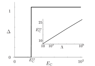
Figure 1: Particle-hole gap $\Delta$ (unit $\mu_{0}$) as a function of the Coulomb energy $E_{\rm C}$ (unit $\mu_{0}/k_{\rm F}l_{B}$) for the cutoff value $\Lambda=10^{5}$. Inset: dependence of the critical value $E_{\rm C}^{\rm cr}$ on $\Lambda$.

III.2 The particle-particle channel.

Equations (31) and (33) are written in a form which also holds for particle-particle pairing. However, in this case $\cal G$ is the Green function for the Nambu field ${\bf\Phi}^{\dagger}({\bf k},\tau)=\left(\psi^{\dagger}_{\uparrow}({\bf k},\tau),\psi_{\downarrow}({-\bf k},\tau)\right)$. This changes $G_{11},G_{12}$ but leaves $O^{+},O^{-}$ invariant. Due to the strong similarities in the formal approaches of the two cases, we can simply use the previous results. metal02 ; varenna The pair breaking gap is given by

$$\Delta(\epsilon)=\frac{\epsilon\Sigma_{12}(\epsilon)}{\epsilon-\Sigma_{11}(\epsilon)}.$$ (38)

The equation to be solved for $\Delta(0)=\Delta$ is

$$1=\frac{C_{-}}{\Delta^{1/3}}-\frac{1}{2\pi E_{\rm C}}\log^{2}\!\frac{\Delta}{\Lambda E_{\rm C}}=f(\Delta,E_{\rm C},\Lambda)$$ (39)

with $\Delta$ in units of $\mu_{0}$, $E_{\rm C}$ in units of $\mu_{0}/k_{\rm F}l_{\rm B}$, $C_{-}\approx 1.4$ and $\Lambda$ is a cutoff parameter. The solutions are shown in Fig. 2.

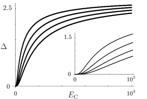
Figure 2: Particle-particle gap $\Delta$ as a function of the Coulomb energy $E_{\rm C}$ for different values of the cutoff $\Lambda$ ($=10^{3},10^{4},10^{5},10^{6}$, top to bottom, units as in Fig. 1). Inset: small-$E_{\rm C}$ behavior.

Here, a solution for $\Delta$ is found for any value of $E_{\rm C}$: nevertheless, values of $\Delta>1$ are not to be accepted because they are outside the range of validity of the assumptions in the calculations.metal02 ; varenna For large $E_{\rm C}$, $\Delta$ is nearly independent of the Coulomb energy and is determined only by the $O^{-}$ contribution, $\Delta=C_{-}^{3}$: this is consistent with the statements in Sec.(II) about the gauge field propagators. In fact, a strong Coulomb interaction quenches the in-phase density fluctuations described by $a^{+}$ and makes the $D^{-}$ contribution even more dominant for $q\to 0$.

III.3 The phase diagram

In order to compare the two pair states one has to compare the gains in their ground state energies with respect to the non-paired state. Equation (27) gives the energy difference between the non-interacting system and the interacting system described by $G$. As we are interested in the difference between the energies of the anomalous state $E$ and the normal interacting system $E_{\rm n}$, we write

$$E-E_{\rm n}=(E-E_{0})-(E_{\rm n}-E_{0})$$

and perform the calculations in (27) twice, first with the full $G$ and then with $G$ for $\Sigma_{12}\to 0$.

III.3.1 Particle-hole ground state energy.

In this case we use the expressions for the imaginary parts in (III.1) and $G_{011}^{-1}(q,\epsilon)=G_{022}^{-1}(q,\epsilon)=\epsilon-q^{2}/2m+\mu$. Performing the $q-$ and $\epsilon-$ integrations we find

$$E-E_{\rm n}=-\frac{m}{2\pi}\int_{0}^{1}\frac{{\rm d}\lambda}{\lambda}\Delta^{2}_{\lambda}.$$

The gap $\Delta_{\lambda}$ is the solution of (37) with an effective interaction $\lambda V^{s,s^{\prime}}_{\mu\nu}$. It can be shown that

$$\Delta_{\lambda}=\lambda\left[\Delta^{+}(\Delta_{\lambda})+\Delta^{-}(\Delta_{\lambda},E_{\rm C},\Lambda)\right].$$ (40)

From the numerical analysis of this, we know that there is a critical value $\lambda^{\rm cr}(E_{\rm C},\Lambda)$ below which $\Delta_{\lambda}=0$, otherwise $\Delta_{\lambda}\approx\mu_{0}$.

To obtain the dependence of the critical parameter on $E_{\rm C}$ and $\Lambda$, we solve (40) for $\lambda^{\rm cr}$ in the limit $\Delta_{\lambda}\to\mu_{0}$. This gives

$$E-E_{\rm n}\approx\frac{m}{2\pi}\Delta^{2}\log\lambda^{\rm cr}.$$ (41)

The energy gain per particle is then

$$\Delta E=\frac{|E-E_{n}|}{\rho}=\frac{\mu_{0}}{2}|\log\lambda^{\rm cr}|.$$ (42)

This is plotted in Fig. 3 as a function of $E_{\rm C}$(thin line). Since $\Delta=0$ for $E_{\rm C}<E_{\rm C}^{\rm cr}(\Lambda)$, $\Delta E=0$ in that region.

III.3.2 Particle-particle ground state energy.

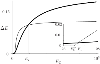
Figure 3: The energy gain $\Delta E$ per particle as a function of $E_{\rm C}$ for $\Lambda=10^{5}$ (units as in Fig. 1). Thick curve: p-p state; thin curve: p-h state. Inset: region near $E_{\rm C}^{\rm cr}$ ($E_{\rm C}^{\rm cr}$ critical energy for p-h pair formation, $E_{1,2}$ energies at which the curves intersect (see text).

In order to use (27) on the p-p channel the components of $G_{0}$ and $G$ are required,

$$G_{011}^{-1}(q,\epsilon)=\epsilon-\xi_{q}\,,\quad G_{022}^{-1}(q,\epsilon)=\epsilon+\xi_{q}$$ (43)

and

$${\rm Im}G_{i}(q,\epsilon) = -\pi\,{\rm sgn}(\epsilon-\Sigma_{11}(\epsilon))\times$$ (44)

$$\times \frac{N_{i}}{2\Omega}\left[\delta(\xi_{q}-\Omega)+\delta(\xi_{q}+\Omega)\right],$$

with index $i$ denoting ${11}$ or ${12}$ and

$$N_{11} = \epsilon-\Sigma_{11}(\epsilon)+\xi_{q}$$

$$N_{12} = \Sigma_{12}(\epsilon).$$

We have here also defined $\Omega=[(\epsilon-\Sigma_{11}(\epsilon))^{2}-\Sigma_{12}(\epsilon)^{2}]^{1/2}$, $\xi_{q}=q^{2}/2m-\mu$ and the off-diagonal component $G_{12}$ has been introduced for later convenience. Since we have neglected the even part of $\Sigma_{11}$, Im$\,G_{11}=$ Im$\,G_{22}$ which also explains why the chemical potential is not modified in the full Green function. Using (38) and the parity properties of $\Sigma_{11},\Sigma_{12}$ one finds

$$E-E_{0}=-\frac{m}{2\pi}\int_{0}^{1}\frac{{\rm d}\lambda}{\lambda}\int_{\Delta_{\lambda}}^{\infty}\!\!\!{\rm d}\epsilon\frac{\epsilon\Sigma_{11}(\epsilon)+\Delta_{\lambda}\Sigma_{12}(\epsilon)}{\sqrt{\epsilon^{2}-\Delta_{\lambda}^{2}}}.$$ (45)

Subtracting the same quantity with $\Delta_{\lambda}\to 0$ gives

$$E-E_{\rm n}\approx\!-\frac{m}{2\pi}\!\!\int_{0}^{1}\!\frac{{\rm d}\lambda}{\lambda}\!\left[\int_{\Delta_{\lambda}}^{\infty}\!\!\!\!{\rm d}\epsilon\frac{\Delta_{\lambda}^{2}}{\epsilon}\!-\!\!\!\int_{0}^{\Delta_{\lambda}}\!\!\!\!{\rm d}\epsilon\Sigma_{11}^{\Delta=0}(\epsilon)\right],$$ (46)

by expanding the integrand in (45) for $\epsilon\gg\Delta_{\lambda}$ and assuming $\Sigma_{11}(\epsilon\gg\Delta_{\lambda})\approx\Sigma_{11}^{\Delta=0}(\epsilon)$. The first part should be integrated with a cutoff $\Lambda_{\rm C}$ and would give a logarithmic contribution $\propto\Delta_{\lambda}^{2}\log\Delta_{\lambda}/\Lambda_{\rm C}$. The most important contributionb99 ; ul94 comes from the second integral that can be evaluated explicitly to the same accuracy taking into account in (33) only $O^{-}$ in the limit $\Delta\to 0$

$$E-E_{\rm n}\approx\frac{m}{2\pi}\int_{0}^{1}\frac{{\rm d}\lambda}{\lambda}\int_{0}^{\Delta_{\lambda}}\!\!\!\!\!\!{\rm d}\epsilon\Sigma_{11}^{-}(\epsilon).$$ (47)

In the same limitmetal02

$$\int{\rm d}q{\rm Im}G_{11}(q,\epsilon_{1}) = -\frac{\pi m}{k_{\rm F}}$$ (48)

and

$$\int_{0}^{\Delta_{\lambda}}\!\!\!\!\!\!{\rm d}\epsilon\Sigma_{11}^{-}(\epsilon)=A^{-}\frac{27\pi m}{5k_{\rm F}}\Delta_{\lambda}^{5/3}=B^{-}\mu_{0}^{1/3}\Delta_{\lambda}^{5/3},$$ (49)

using the notations of (A) for the value of the constant $A^{-}$ and implicitly defining the numerical constant $B^{-}$.

The energy gain per particle is then

$$\Delta E=\frac{\mu_{0}}{2}\,|B^{-}|\int_{0}^{1}\frac{{\rm d}\lambda}{\lambda}\left(\frac{\Delta_{\lambda}}{\mu_{0}}\right)^{5/3}.$$ (50)

The final step has been then performed numerically with the self-consistency equation (39) modified according to $1=\lambda f(\Delta_{\lambda},E_{\rm C},\Lambda)$. The results are shown in Fig. 3 (bold curve).

III.3.3 Phase diagram.

Figure 3 shows that the curves for $\Delta E$ corresponding to the two models intersect at certain energies $E_{1}(\Lambda)$ and $E_{2}(\Lambda)$. These energies separate the regions of stability of excitonic and Cooper pair phases.

It is useful to recall the validity of the assumptions made in the calculations. First, the validity of a mean-field treatment of the interaction has to be addressed. It has been shownSternHalp95 that in the normal state the dominant contribution of the gauge field propagator is not expected to be renormalized by vertex corrections. It is not clear whether or not this approximation still holds in the anomalous states.Khves93 For approaching the paired state from the normal state, we believe that neglecting vertex corrections, and using the bare vertices (17) in (24) is at least a reasonable starting point. Second, earlier calculationsmetal02 show that the particle-particle energy gap survives the linearization of the dispersion law of the fermions around the Fermi level. However, for the particle-hole channel it is necessary to keep a higher accuracy and take the full quadratic dependence of $\xi_{q}$ on $q$ into account (cf. (71)).

For energies $E_{1}<E_{\rm C}<E_{2}$ it is more favorable to form a p-h state, while for $E_{\rm C}<E_{1}$ and $E_{\rm C}>E_{2}$ the formation of a p-p state is energetically favorable. The dependence on the value of the cutoff of the threshold energies is shown in Fig. 4. Light grey regions corresponds to the p-p states. The dashed line corresponds to the values of $E_{\rm C}$ such that the p-p pair breaking gap equals $\mu_{0}$. Due to the approximations used in the calculations of the p-p gap, only the part of the graph to the left of this curve can be expected to describe correctly the system.

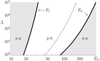
Figure 4: The phase diagram for the ground state in the plane of the Coulomb energy $E_{\rm C}$ and the cutoff parameter $\Lambda$. Light grey region: the p-p state; white region: p-h state. Dashed: $E_{\rm C}(\Delta=\mu_{0})$ for the p-p state.

IV Short-range interaction

The possibility of a crossover between an excitonic and a superconducting CF state has been demonstrated for long range Coulomb interaction. In this section we want to investigate whether or not this is a generic feature of any interaction. We consider an interaction potential of the form introduced in Section (II.1),

$$V(q)=\frac{2\pi e^{2}}{\epsilon\sqrt{q^{2}+1/r_{0}^{2}}}.$$

It has been pointed out above that in this case one must treat the in-phase and out-of-phase gauge field fluctuations $D^{+}$ and $D^{-}$ on the same footing. By defining $V_{0}=V(q\to 0)=2\pi e^{2}r_{0}/\epsilon$ and $\alpha_{+}^{\prime}=\alpha_{+}/q=V_{0}/\phi_{0}^{2}$ one obtains for the bosonic propagators

$${\cal D}^{+}_{11}({\bf q},\Omega_{n}) \approx \frac{-q}{(\alpha_{+}^{\prime}+\alpha_{-})\,q^{3}+\eta\,|\Omega_{n}|}$$

$${\cal D}^{-}_{11}({\bf q},\Omega_{n}) \approx \frac{-q}{\alpha_{-}\,q^{3}+\eta\,|\Omega_{n}|}\,.$$ (51)

Thus one proceeds along the line of the calculations done for long-range interaction for the case of $D^{-}$.

IV.1 The particle-hole state

To find the gap we have to solve (33) for $\Sigma_{12}$, but now $O^{\pm}$ have to be calculated according to (A) with ${\cal D}^{\pm}$ in (IV). For the real parts one gets

$$O^{\pm}(\epsilon,\epsilon_{1}) = A^{\pm}_{\rm sr}\,\frac{1+3\,{\rm sgn}\epsilon_{1}\,{\rm sgn}(\epsilon_{1}-\epsilon)}{(\epsilon-\epsilon_{1})^{1/3}}$$ (52)

with

$$A^{-}_{\rm sr} = C\frac{\pi^{2}}{9}\frac{1}{\alpha_{-}^{2/3}\eta^{1/3}}$$

$$A^{+}_{\rm sr} = C\frac{\pi^{2}}{9}\frac{1}{(\alpha_{+}^{\prime}+\alpha_{-})^{2/3}\eta^{1/3}}=A^{-}_{\rm sr}\left(1+\frac{\alpha_{+}^{\prime}}{\alpha_{-}}\right)^{-2/3}$$

and $C$ in (64).

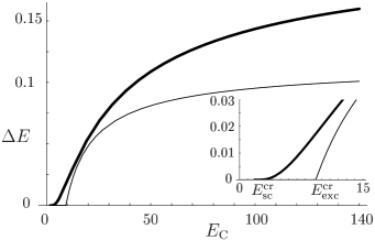
Figure 5: The energy gain $\Delta E$ per particle (units $\mu_{0}$) for short range interaction as a function of $E_{\rm C}$ (units $4\mu_{0}l_{B}/3r_{0}(k_{\rm F}l_{B})^{2}$); p-p state (bold curve), p-h state (thin curve). Inset: the region near $E_{\rm sc}^{\rm cr}$and $E_{\rm exc}^{\rm cr}$.

The integrals which one has to evaluate have the same structure as for $\Delta^{-}$ [cf. (A)] in the long-range case. The result is very similar and the self-consistency equation is (for $\Delta<\mu_{0}$)

$$\Delta=K^{-}A\,\Gamma^{<}\Big{[}(\mu_{0}+\Delta)^{1/6}-(\mu_{0}-\Delta)^{1/6}\Big{]}$$ (53)

with the prefactor

$$A=1-\left(1+\frac{\alpha_{+}^{\prime}}{\alpha_{-}}\right)^{-2/3}$$

and the constants $K^{-},\Gamma^{<}$ of (A, 74). It can be seen by numerical evaluation that this equation has always a solution ($\approx\mu_{0}$) if

$$9.3\approx r_{\rm cr}<r=\frac{\alpha_{+}^{\prime}}{\alpha_{-}};$$

since

$$r=(k_{\rm F}l_{B})^{2}\frac{3}{4}\frac{E_{\rm C}}{\mu_{0}}\frac{r_{0}}{l_{B}},$$ (54)

from the last inequality we define a critical value $E_{\rm exc}^{\rm cr}$ for the Coulomb energy $E_{\rm C}$ below which $\Delta=0$ as in the long-range limit (cf. Fig. 4, 5).

The ground state energy gain per particle can be estimated along the same line of (III.3.1): the result is as in (42)

$$\Delta E=\frac{\mu_{0}}{2}|\log\lambda^{\rm cr}_{\rm sr}|$$ (55)

but with a critical parameter $\lambda_{\rm sr}^{\rm cr}$ obtained from the solution of (40) with the short-range form of $\Delta^{+},\Delta^{-}$:

$$\lambda^{\rm cr}_{\rm sr}\approx\frac{0.79}{A}.$$ (56)

IV.2 The particle-particle state

It has been shown previouslyvarenna that by substituting the appropriate Green functions (44), the two equations (33) can be combined according to (38) to yield a self-consistency equation for $\Delta$, similar to (39) but without the $\log^{2}$ term due to the Coulomb interaction. Combining these results one finds

$$1=C_{-}\left(\frac{\Delta}{\mu_{0}}\right)^{-1/3}\left[1-2\left(1+\frac{\alpha_{+}^{\prime}}{\alpha_{-}}\right)^{-2/3}\right],$$ (57)

where

$$C_{-}=-\frac{2m\pi}{k_{\rm F}}\frac{8}{3}A^{-}_{\rm sr}\frac{3\sqrt{\pi}\Gamma(7/6)}{\Gamma(2/3)}\,\mu_{0}^{-1/3}\approx 1.4$$

is the same as in (39) and the prefactor reflects the competition of the $O^{\pm}$ contributions. A critical value for the ratio $r$ exists also in this case due to the requirement that $\Delta>0$; one has $r>2^{3/2}-1$. This defines a critical value $E_{\rm sc}^{\rm cr}$ according to (54); for $E_{\rm C}<E_{\rm sc}^{\rm cr}$ the gap equation has no solutions. Otherwise, the gap is an increasing function of $r$ starting from $\Delta=0$ and reaching $\Delta=1$ for $r\approx 16.8$. Equation (47) and the following one provide the estimate for the ground state energy difference,

$$E-E_{\rm n}=B^{-}\mu_{0}^{1/3}\frac{m}{2\pi}\left(1+(1+r)^{-2/3}\right)\int_{0}^{1}\frac{{\rm d}\lambda}{\lambda}\Delta_{\lambda}^{5/3}$$ (58)

where $B^{-}\approx-0.39$ is the same as in the Coulomb case since the antisymmetric propagator is not affected by the range of the interaction. The index $\lambda$ in $\Delta_{\lambda}$ has the usual meaning: equation (57) with a factor $\lambda$ added to the right hand side can be used to obtain explicitly $\Delta_{\lambda}$. The energy gain per particle is

$$\Delta E=|B^{-}|\frac{\mu_{0}}{2}\frac{C_{-}^{5}}{5}\left[1+(1+r)^{-\frac{2}{3}}\right]\left[1-2(1+r)^{-\frac{2}{3}}\right]^{5}.$$ (59)

The result is shown in Fig. 5 as a function of $E_{\rm C}$ (bold curve). Within the present approximations, the two curves for the p-p state and the p-h state do not intersect. The energy gain per particle for the p-p state is always larger than for the p-h state if the interaction is short ranged. The excitonic state is always suppressed in favour of the Cooper pair-like state.

V Conclusions

We have investigated in this paper whether or not the residual interaction due to fluctuations of the CS gauge field between CFs with spin at filling factor 1/2 can lead to the formation of new collective ground state. We have assumed that fluxes and Fermions corresponding to the same spins are coupled via the CS transformation. We take into account the renormalization of the propagator of the gauge field due to the coupling to the Fermions. The dominant effective interaction between the CFs is then of second order in the gauge field-electron vertex and we have found that it can be attractive between CFs with opposite spins. Thus, the formation of pairs is possible, which we have investigated in the spin singlet, s-wave channel.

We have estimated both the pair-breaking gaps and the ground state energies of particle-particle and particle-hole channels for long-range Coulomb and finite range interactions. We find that in the former case both, the particle-particle as well as the particle-hole state can be stable depending on the strength of the interaction. The particle-particle state is stable if the Coulomb energy is smaller than a certain threshold energy (which depends on a cutoff parameter). For higher Coulomb energy, the excitonic state is favored. If the interaction is screened, symmetric and antisymmetric density fluctuations, as described by $D^{+}$ and $D^{-}$, become comparable and the particle-particle state is always more stable than the particle-hole state.

The formation of these states has been shown to be possible if the spin $\uparrow$ and the spin $\downarrow$ Landau levels are degenerate and both of them exactly at filling factor 1/2. One can suspect that the results remain valid also if these conditions are not exactly fulfilled. If the two Landau levels are not degenerate the new ground state will form as long as the energy separation between the two levels is smaller than the gain in the ground state energy. Assume the level with spin $\uparrow$ to be energetically lower. Then, the ground state without interaction corresponds to this level completely filled. With interaction (i.e. with gauge field fluctuations), however, the instabilities discussed in the present paper would be present and half of the electrons would occupy the (energetically higher) level with spin $\downarrow$ such that the energetically more favorable collective ground state can be achieved by forming spin singlet particle-particle or particle-hole pairs. The situation in which each of the two levels is exactly at $\nu=1/2$ is then the ground state since any deviation from this occupation would yield a higher energy. This mechanismvarenna would be relevant in the interpretation of the intermediate plateaus in the optical measurements of spin polarizationKukushkin for both the p-p and the p-h pairings; thus further experimental investigation would be necessary to test the actual interplay between the two proposed phases.

*

Appendix A Details of calculations

In the evaluation of the integrals we use similar results for the Cooper channel.pss In order to perform the ${\bf q}$-integration in Eq. (III.1) and get the form in Eq.(33), we rewrite the expression for the vertices with $p=|{\bf k-q}|$,

$$\frac{({\bf k}\times{\bf q})^{2}}{|{\bf k}-{\bf q}|^{2}}=\frac{k^{2}q^{2}}{p^{2}}\sin^{2}\theta$$ (60)

where $\theta$ is the angle between ${\bf k}$ and ${\bf q}$. Aligning the $q_{x}$ axis along the $\hat{k}$ direction, the measure is changed

$$\int_{0}^{\infty}\!\!q{\rm d}q\int_{0}^{2\pi}\!\!{\rm d}\theta=2\int_{0}^{\infty}\!\!{\rm d}q\int_{|k-q|}^{k+q}\!\!\frac{p{\rm d}p}{k\sin\theta}$$ (61)

with

$$\sin\theta=\left[1-\Big{(}\frac{k^{2}+q^{2}-p^{2}}{2kq}\Big{)}^{2}\right]^{1/2}\,.$$ (62)

If we assume for the external momentum $k\approx k_{\rm F}$ and consider only the dominant contribution with $q\sim k_{\rm F}$, we get for $\Sigma_{ij}(\epsilon)\approx\Sigma_{ij}(k_{\rm F},\epsilon)$ ($i=1,j=1,2$)

$$\Sigma_{ij}(\epsilon) = C\int_{0}^{\infty}\!\!{\rm d}q\int_{0}^{2k_{\rm F}}\!\!\!\!{\rm d}p\sqrt{1-\frac{p^{2}}{4k_{\rm F}^{2}}}\times$$ (63)

$$\times\int_{-\infty}^{+\infty}\!\!\!\!{\rm d}\omega{\rm d}\epsilon_{1}({\rm sgn}\epsilon_{1}+{\rm sgn}\omega){\rm Im}G_{ij}(q,\epsilon_{1})\times$$

$$\times\frac{{\rm Im}\left[D_{11}^{+}({p},\omega)+(-1)^{i+j}D_{11}^{-}({p},\omega)\right]}{\omega+\epsilon_{1}-\epsilon-i\delta}$$

with the constant

$$C=-\frac{e^{2}k_{\rm F}^{2}}{4\pi^{4}m^{2}}.\\$$ (64)

In order to obtain (33) we then have

$$O^{\pm}(\epsilon,\epsilon_{1}) = C\int{\rm d}p\int{\rm d}\omega({\rm sgn}\epsilon_{1}+{\rm sgn}\omega)$$ (65)

$$\qquad\times\frac{{\rm Im}D^{\pm}_{11}(p,\omega)}{\omega+\epsilon_{1}-\epsilon-i\delta}.$$

Assuming $p\ll k_{\rm F}$ the $p$-integral can be performed,

$${\rm Im}D_{11}^{\pm}(p,\omega)=\frac{-\eta\omega p}{\alpha_{\pm}^{2}p^{(5\mp 1)}+\eta^{2}\omega^{2}}$$ (66)

and

$$\int_{0}^{\infty}{\rm d}p\,{\rm Im}D_{11}^{+}(p,\omega) = -\frac{\pi}{4\alpha_{+}}{\rm sgn}\omega\,,$$

$$\int_{0}^{\infty}{\rm d}p\,{\rm Im}D_{11}^{-}(p,\omega) = -\frac{\pi}{3\sqrt{3}}\frac{1}{\alpha_{-}^{2/3}\eta^{1/3}\omega^{1/3}}.$$

Now the energy integrations have to be performed as principal value integrals. We have

$$O^{+}(\epsilon,\epsilon_{1}) = A^{+}\left[\log\frac{|\Lambda_{\rm C}+\epsilon_{1}-\epsilon|}{|\Lambda_{\rm C}-\epsilon_{1}+\epsilon|}+{\rm sgn}\epsilon_{1}\log\frac{|\Lambda_{\rm C}^{2}-(\epsilon_{1}-\epsilon)^{2}|}{|(\epsilon_{1}-\epsilon)^{2}|}+i\pi(1-{\rm sgn}\epsilon_{1}\,{\rm sgn}(\epsilon_{1}-\epsilon))\right],$$

$$O^{-}(\epsilon,\epsilon_{1}) = A^{-}\left[\frac{1+3\,{\rm sgn}\epsilon_{1}\,{\rm sgn}(\epsilon_{1}-\epsilon)}{(\epsilon-\epsilon_{1})^{1/3}}-i\sqrt{3}\frac{{\rm sgn}\epsilon_{1}+{\rm sgn}(\epsilon-\epsilon_{1})}{(\epsilon-\epsilon_{1})^{1/3}}\right],$$ (68)

with the constants

$$A^{+} = -C\frac{\pi}{4\alpha_{+}}$$

$$A^{-} = C\frac{\pi^{2}}{9}\frac{1}{\alpha_{-}^{2/3}\eta^{1/3}}$$ (69)

and a cutoff $\Lambda_{\rm C}$ that must be introduced to evaluate $O^{+}$. A physically meaningful value for this can be estimated by considering in more detail the integral

$$\int_{0}^{2k_{\rm F}}{\rm Im}D^{+}_{11}(p,\omega)=-\frac{1}{2\alpha_{+}}\left(\frac{\pi}{2}-\arctan\frac{\eta\omega}{4k_{\rm F}^{2}\alpha_{+}}\right).$$

This vanishes for $\omega\to\infty$. The scale for the vanishing of the integral can be obtained by considering the argument of the $\arctan$

$$\frac{\eta\omega}{4k_{\rm F}^{2}\alpha_{+}}=\frac{\omega}{E_{\rm C}}\frac{1}{2k_{\rm F}l_{\rm B}}$$ (70)

where $E_{\rm C}=e^{2}/\epsilon l_{\rm B}$. From this, it is reasonable to choose as the cutoff $\Lambda_{\rm C}=\Lambda k_{\rm F}l_{\rm B}E_{\rm C}$, where $\Lambda$ represents the numerical value of the cutoff.

Next step is to consider the contribution from the fermionic Green function: the $q$-integrals for the diagonal part, Im$G_{11}$, and the off-diagonal part, Im$G_{12}$, yield

$$\Theta^{ij}(\epsilon) \equiv \int\!\!{\rm d}q{\rm Im}G_{ij}(q,\epsilon)=$$ (71)

$$= -\frac{\pi}{2}\sqrt{\frac{m}{2}}\left[\frac{\theta(\epsilon+\overline{\mu}-\Delta)}{\sqrt{\epsilon+\overline{\mu}-\Delta}}\right.+$$

$$+(-1)^{i+j}\left.\frac{\theta(\epsilon+\overline{\mu}+\Delta)}{\sqrt{\epsilon+\overline{\mu}+\Delta}}\right]$$

This gives finally for the self-energies

$$\Sigma_{ij}(\epsilon)=\int_{-\infty}^{+\infty}{\rm d}\epsilon_{1}\Theta^{ij}(\epsilon_{1})\left[O^{+}(\epsilon,\epsilon_{1})+(-1)^{i+j}O^{-}(\epsilon,\epsilon_{1})\right].$$ (72)

We now concentrate on the $\epsilon_{1}$-integral for $\Delta=\Sigma_{12}$ in the limit $\epsilon\to 0$. We first realize that the imaginary parts of $O^{+}$ and $O^{-}$ do not contribute. The main contribution comes from Re$\,O^{-}$ and, with the notation of (37),

$$\Delta^{-}=-\int{\rm d}\epsilon_{1}\Theta^{12}(\epsilon_{1})O^{-}(\epsilon\to 0,\epsilon_{1}).$$

The latter integral can be solved in the two regimes $\Delta\lessgtr\overline{\mu}$. One finds

$$\begin{array}[]{clc}\Delta^{-}=&K^{-}\Gamma^{<}\left[(\overline{\mu}+\Delta)^{1/6}-(\overline{\mu}-\Delta)^{1/6}\right]&(\Delta<\overline{\mu})\\ &&\\ \Delta^{-}=&K^{-}\Big{[}\Gamma^{>}(\Delta-\overline{\mu})^{1/6}+\Gamma^{<}(\Delta+\overline{\mu})^{1/6}\Big{]}&\,(\Delta>\overline{\mu})\end{array}$$

with the constants $\Gamma^{>},\Gamma^{<}$ defined in terms of Euler gamma function $\Gamma$

$$\Gamma^{<} = \Gamma\left(\frac{2}{3}\right)\left(\frac{\sqrt{\pi}}{\Gamma(7/6)}-\frac{\Gamma(-1/6)}{\sqrt{\pi}}\right)\approx 7.76$$

$$\Gamma^{>} = \frac{\sqrt{\pi}\Gamma(-1/6)}{\Gamma(1/3)}\approx-4.48$$ (73)

and

$$K^{-} = -4\frac{\pi}{2}\sqrt{\frac{m}{2}}A^{-}\approx 0.15\mu_{0}^{5/6}.$$ (74)

These must be combined with the corresponding relations for $\overline{\mu}=\overline{\mu}(\Delta)$ of (36) to obtain a self-consistency equation for $\Delta$. Neglecting for the moment the contribution of $O^{+}$, we have for $\Delta<1$

$$\Delta=1.13\left((1+\Delta)^{1/6}-(1-\Delta)^{1/6}\right)$$

where $\Delta$ is expressed in units of $\mu_{0}$. The solution to this equation is indeed very close to $\mu_{0}$ itself.

The inclusion of $O^{+}$ implies the solution of a more complicated integral

$$\Delta^{+}=\int{\rm d}\epsilon_{1}\Theta^{12}(\epsilon_{1})O^{+}(\epsilon\to 0,\epsilon_{1}).$$

It can be solved analytically and it is possible to show that it only shifts the solution even closer to $\mu_{0}$. The most important effect of considering the $O^{+}$ integral is, however, that it introduces a new energy scale $E_{\rm C}$ and a cutoff parameter $\Lambda$. The value of the gap is largely independent from $E_{\rm C}$, but depending on the cutoff there exists a critical value $E_{\rm C}^{\rm cr}(\Lambda)$ of the Coulomb energy below which there are no solutions to the equation $\Delta=\Delta^{+}+\Delta^{-}$ (see Fig.  1).

- (1) J. K. Jain, Phys. Rev. Lett. 63, 199 (1989).
- (2) A. Stern and B. I. Halperin, Phys. Rev. B 52, 5890 (1995).
- (3) A. Lopez and E. Fradkin, Phys. Rev. B 44, 5246 (1991).
- (4) B. I. Halperin, P. A. Lee, and N. Read, Phys. Rev. B 47, 7312 (1993).
- (5) Composite Fermions , edited by O. Heinonen (World Scientific 1998).
- (6) R. L. Willett, Adv. Phys. 46, 447 (1997) and references therein.
- (7) R. L. Willett, R. R. Ruel, K. W. West, and L. N. Pfeiffer, Phys. Rev. Lett. 71, 3846 (1993).
- (8) W. Kang, H. L. Stormer, L. N. Pfeiffer, K. W. Baldwin, and K. W. West, Phys. Rev. Lett. 71, 3850 (1993)
- (9) I. V. Kukushkin, J. H. Smet, K. von Klitzing, and W. Wegscheider, Nature 415, 409 (2002).
- (10) J. G. Bednorz and K. A. Müller, Z. PHys. B 64,189 (1986)
- (11) N. Grewe and F. Steglich, in Handbook on the Physics and Chemistry of Rare Earths, ed. by K. A. Geschneider and L. Eyring (North Holland, Amsterdam 1991); M. B. Maple, cond-mat/9802202.
- (12) S. V. Kravchenko and M. P. Sarachik, Rep. Prog. Phys. 67, 1 (2003).
- (13) R. G. Clark, S. R. Haynes, A. M. Suckling, J. R. Mallett, P. W. Wright, J. J. Harris, and C. T. Foxon, Phys. Rev. Lett. 62, 1536 (1989).
- (14) J. P. Eisenstein, H. L. Stormer, L. N. Pfeiffer, and K. W. West, Phys. Rev. Lett. 62, 1540 (1989).
- (15) J. P. Eisenstein, H. L. Stormer, L. N. Pfeiffer, and K. W. West, Phys. Rev. B 41, 7910 (1990).
- (16) L. W. Engel, S. W. Hwang, T. Sajoto, D. C. Tsui, and M. Shayegan, Phys. Rev. B 45, 3418 (1992).
- (17) I. V. Kukushkin, K. von Klitzing, and K. Eberl, Phys. Rev. Lett. 82, 3665 (1999); I. V. Kukushkin, K. von Klitzing, K. G. Levchenko, and Yu. E. Lozovik, JETP Letters 70, 730 (1999); I. V. Kukushkin, J. H. Smet, K. von Klitzing, and K. Eberl, Phys. Rev. Lett. 85, 3688 (2000).
- (18) E. Mariani, R. Mazzarello, M. Sassetti, and B. Kramer, Ann. Phys. (Leipzig) 11, 926 (2002).
- (19) N. Freytag, Y. Tokunaga, M. Horvatić, C. Bertier, M. Shayegan, and L. P. Levy, Phys. Rev. Lett. 87, 136801 (2001).
- (20) W. Pan, H. L. Stormer, D. C. Tsui, L. N. Pfeiffer, K. W. Baldwin, and K. W. West, Phys. Rev. Lett. 90, 016801 (2003).
- (21) A most recent review has been compiled by G. Murthy and R. Shankar, Rev. Mod. Phys. 75, 1101 (2003).
- (22) G. Murthy, Phys. Rev. Lett. 84, 350 (2000).
- (23) V. M. Apalkov, T. Chakraborty, P. Pietilainen, and K. Niemela, Phys. Rev. Lett. 86, 1311 (2001).
- (24) K. Park and J. K. Jain, Phys. Rev. Lett. 80, 4237 (1998).
- (25) A. Lopez and E. Fradkin, Phys. Rev. B 63, 085306 (2001).
- (26) S. S. Mandal and V. Ravishankar, Phys. Rev. B 54, 8688 (1996).
- (27) Y. B. Kim, C. Nayak, E. Demler, N. Read, and S. Das Sarma, Phys. Rev. B 63, 205315 (2001).
- (28) T. Morinari, Phys. Rev. B 65, 115319 (2002); 59, 7320 (1999).
- (29) B. I. Halperin, Helv. Phys. Acta 56, 75 (1983); Surf. Sci. 305, 1 (1994).
- (30) M.Y. Veillette, L. Balents, and M.P.A. Fisher, Phys. Rev. B 66, 155401 (2002).
- (31) J. Ye, cond-mat/0302558.
- (32) I. B. Spielman, J. P. Eisenstein, L. N. Pfeiffer, and K. W. West, Phys. Rev. Lett. 84, 5808 (2000)
- (33) R. Rajaraman and S. L. Sondhi, Int. J. Mod. Phys. B 10, 793 (1996).
- (34) T. Morinari, Phys. Rev. B 62, 15903 (2000).
- (35) E. Mariani, N. Magnoli, F. Napoli, M. Sassetti, and B. Kramer, Phys. Rev. B 66, 241303 (2002).
- (36) B. Kramer, E. Mariani, N. Magnoli, M. Merlo, F. Napoli, and M. Sassetti, Phys. Status Solidi B 234, 221 (2002).
- (37) B. Kramer, N. Magnoli, E. Mariani, M. Merlo, F. Napoli, and M. Sassetti, in Quantum Phenomena in Mesoscopics Physics, proceedings of the International School of Physics Enrico Fermi, Varenna, 2002 edited by A. Tagliacozzo, B. Altshuler, and V. Tognetti, 2003.
- (38) N. E. Bonesteel, I. A. McDonald, and C. Nayak, Phys. Rev. Lett. 77, 3009 (1996).
- (39) A. Abrikosov, L. Gorkov, and I. Dzyaloshinski, Methods of quantum field theory in statistical physics (Prentice Hall, Englewood Cliffs NJ, 1963).
- (40) G. M. Eliashberg, Zh. Eksp. Teor. Fiz. 39, 1437 (1960) [Sov. Phys. JETP 12, 1000 (1961)].
- (41) D. V. Khveshchenko, Phys. Rev. B 47, 3446 (1993).
- (42) N. Nagaosa and P. A. Lee, Phys. Rev. Lett. 64, 2450 (1990).
- (43) N. E. Bonesteel, Phys. Rev. Lett. 82, 984 (1999).
- (44) M. U. Ubbens and P. A. Lee, Phys. Rev. B 49, 6853 (1994).