Causal Slaving of the U.S. Treasury Bond Yield Antibubble by the Stock Market Antibubble of August 2000

Abstract

Using the descriptive method of log-periodic power laws (LPPL) based on a theory of behavioral herding, we use a battery of parametric and non-parametric tests to demonstrate the existence of an antibubble in the yields with maturities larger than 1 year since October 2000. The concept of “antibubble” describes the existence of a specific LPPL pattern that is thought to reflect collective herding effects. From the dependence of the parameters of the LPPL formula as a function of yield maturities and using lagged cross-correlation calculations between the S&P 500 and bond yields, we find strong evidence for the following causality: Stock Market $\to$ Fed Reserve (Federal funds rate) $\to$ short-term yields $\to$ long-term yields (as well as a direct and instantaneous influence of the stock market on the long-term yields). Our interpretation is that the FRB is “causally slaved” to the stock market (at least for the studied period), because the later is (taken as) a proxy for the present and future health of the economy.

,

1 Introduction

Since August 2000 until the end of 2002, the USA as well as most other western markets have depreciated almost in synchrony according to complex patterns of drops and local rebounds. We have proposed to describe this phenomenon using the concept of a log-periodic power law (LPPL) “antibubble,” characterizing behavioral herding between investors leading to a competition between positive and negative feedbacks in the pricing process [1, 2, 3, 4, 5]. The concept of an “antibubble” was inspired by that of an “antiparticle” in physics. Just as an antiparticle is identical to its sister particle except that it carries exactly opposite charges and destroys its sister particle upon encounters, an antibubble is both the same and the opposite of a bubble; it’s the same because similar herding patterns occur, but with a bearish vs. bullish slant. Our work on antibubbles is thus the counterpart of a large research effort that we and others have developed to characterize speculative bubbles (see [6, 7, 8, 9] and references therein).

However, in addition to imitative and herding behavior, one quantifiable factor that many analysts and traders think plays an important role in the development of both bubbles and antibubbles is the influence of the Federal Reserve Board’s (FRB) liquidity interventions into the financial markets. On a daily basis, the Federal Reserve intervenes to adjust short-term interest rates. Through open market operations, the FRB buys and sells U.S. Government securities (variously-termed Treasury instruments having term periods that range from overnight to a couple of weeks) in the secondary market in order to adjust the level of reserves in the banking system. By adjusting the level of reserves in the banking system through their buys or sells which modulate the supply-demand equation, the FRB can offset or support seasonal or cyclical shifts of funds and thereby affect short-term interest rates and the growth of the money supply, thus effecting the cost of borrowing in the larger economy.

The impact of the FRB does not stop with the short-term interest rates but spreads to bonds (mechanically) and to the stock markets through several channels. One particularly simple channel is the influence of the risk-free interest rates on the present value of discounted future earnings and dividends. The interest rates, as the prices or costs of money at different time horizons, are affected by production opportunities, time preference for consumption, risk and expected inflation. The FRB uses a model of the U.S. economy to shape its decisions that takes into account the monetary transmission mechanism, that is, how its monetary policy actions influence financial markets and aggregate output and inflation [10]. By its interventions, the FRB puts or removes short-term liquidity into the hands of bankers who use it to invest in or desinvest from various financial instruments including equities. This would obviously have an influence on near-term market move directions. One can argue that the FRB intervenes in the stock markets by this indirect mean. An example of extraordinary action by the FRB was in the months prior to the turn of the Millennium. At the time, the Fed reported their intent to ameliorate possible liquidity problems on January 1, 2000 by the injection of several hundred billion dollars. Many believe that this liquidity was a substantial factor in early doubling the value of the Nasdaq stock market into the first quarter of 2000. Another extreme example is, in the week following September 11, 2001, when the Fed reported Open Market Operations activity of $76 billion, one of the single largest weekly liquidity doses in recent history. In August 2003, in response to the power outages of the Northeast and Canada, the FRB’s market intervention peaked to $48 billion in a single day in total outstanding repurchase agreements, an amount approximately equal to that needed to rebuild the flawed electrical power grid in America. Based on comparison between the net value of outstanding Fed repurchase agreements (repo) and financial indices such as the S&P 500 index, some analysts have suggested a correlation between the dips of the market and the ramping up of FRB repo activities, implying a causal relationship in which the FRB influences the stock market (see for instance http://www.piraz.com/monetary/temp99b.gif). An interesting suggestion is that the FRB would appear to inject liquidity to the market not in a steady–state fashion but only at those times when its action may have a strong impact. The rational for this is based on the recognition that many Americans engaged themselves economically through the financial markets in the late 1990s and the capitalization of the US stock market is now significantly larger than the US GDP. There is temptation to view the stock markets as leading the economy. Knowledgeable investors and traders then understand that the FRB acts accordingly to use liquidity to push the markets and, thus, push the economy.

In contrast to this arrow of causality in which it is the FRB which influences the stock market, others suggest the opposite direction of causality, namely, that the monetary policy reacts to the stock markets. However, the magnitude of the FRB’s reaction to the stock market is very hard to estimate in part because of the simultaneous response of equity prices to interest rates [11]. The near-term path of the FRB’s policy might respond to equity price movements due to the direct wealth effect (a higher stock market spill over to increase consumption) and because the stock market prices might contain information on the future economic activity (the current prices are thought to reflect expectations of future earnings and dividends). Rigobon and Sack have found evidence for a significant monetary policy response to the stock market, using an identification technique based on the heteroskedasticity of the stock market returns applied to daily S&P 500 index data running from March 1985 to December 1999 [11]. Their method consists in conditioning the covariance matrix between stock market returns and the three-month treasury bill interest rate on different volatility levels in order to identify the impact of volatility regimes. Bohl, Siklos and Werner [12] argued that the Bundesbank reacted to the stock market systematically on one month scale (or lower frequency), although the effect is not significant.

This question is embedded within a broader question: what is the information content of interest rate time series and of the shape of the yield curve ? Empirically, it has been shown that interest rate spreads have predictive power for the real economic activity and for inflation. For many countries, the interest spreads seem to outperform other leading financial indicators [16, 17, 18, 19, 20, 21, 22, 23]. This is over controversial: financial variables are sometimes argued not to predict real activities [24, 25] while leading economic indicators do have predictive power [26, 27]. There is also evidence that the interest rates and their spreads variables could potentially be used as leading indicators for real estate markets [28]. Yield spreads have been used successfully to forecast the US recession in 2001 [29, 30, 31], which occurred about a year after the “new economy” bubble burst. With respect to the stock market, Roehner has found strong negative correlations between stock market crash-recovery and interest rate spread [32], while Resnick and Shoesmith showed that the interest rates spread between the yields of US composite 10-year+ US T-bond and three-month T-bill carries informative content of a forthcoming bear market one month in advance [33]. In contrast, the interest rates (or bond yields) have been argued to have no significant forecasting ability [34]. This suggests that the arrow of causality goes from the interest rates to the stock market, consistent with the above idea that the FRB may influence the stock market through its monetary policy.

Here, we provide a novel approach to this topic by analyzing the FRB’s reaction to the stock market after the 2000 crash. Our methodology is more efficient than previous works because we use a first-order deterministic indicator rather than second-order covariance measures. Our study also capitalizes on the rather unique setting since 2000 provided by the stock market on the one hand and by the FRB’s monetary policy on the other hand and on our ability to model quantitatively these behaviors. First, we identify specific log-periodic power law (LPPL) signatures in the treasury security yields. Specifically, Sec. 2 presents our LPPL analysis of the US treasury securities yields, which shows that an antibubble also started in October 2000 on the yields with maturities of 2 years or larger. Section 3 strengthens the evidence for log-periodicity by demonstrating the existence of a strong third harmonic in the log-periodicity. Section 4 shows the existence of antibubbles within antibubbles in the time dependence of the long-maturity yields since 1979. Section 5 demonstrates the existence of a log-periodic pattern in the timing of the moves of the Federal funds rate. In other words, the times at which the FRB lowered its leading indicator are organized according to an approximate geometric series with accumulation time (going backward) around October 2000. Section 6 shows that the pattern of timing of the FRB action closely matches that of significant drops in the stock market with an average time lag of about 1-2 months. In addition, the critical time $t_{c}$ of the antibubble LPPL patterns of the interest rate time series are found all approximately three months after that the critical time of the stock market antibubble. This strongly suggests that the FRB’s actions reacted to the stock market rather than the reverse. Section 7 concludes.

2 Evidence of an antibubble structure in the time evolution of U.S. Treasury bond yields

2.1 The LPPL antibubble framework and its calibration

We use the theory characterizing behavioral herding between investors in terms of a competition between positive and negative feedbacks in the pricing process, which has been documented in [6, 7, 8]. Specifically, we refer to the parametrization [35, 2] adapted to the description of antibubbles under the form:

$$y\left(t\right)=A+\left(t-t_{c}\right)^{m}\left\{B+\sum_{n=1}^{N}C_{n}\cos\left[n\omega\ln\left(t-t_{c}\right)-\phi_{n}\right]\right\}+\epsilon(t)~{},$$ (1)

where $t_{c}$ is the theoretical inception time of the antibubble and $\epsilon(t)$ is a white noise residue. The first-order ($N=1$) and second-order ($N=2$) formulae are the versions that have been most used previously in modelling and predicting financial bubbles and antibubbles. We refer to Ref. [7, 8] and references therein for a full exposition of the approach.

Figure 1 shows the evolution with times of ten yields with the maturities 3M, 6M, 1Y, 2Y, 3Y, 5Y, 7Y, 10Y, 20Y, 30Y and of the Federal funds rate since January 2000. As can be seen from the almost simultaneous crossing of all yields in October 2000 which is close to the inception of the 2000 yield antibubble documented below, the yield curve exhibited a rather anomalous inverted shape during the first half of 2000 and resumed its normal upward concave shape after, with a spread between the rates of different maturities broadening with time.

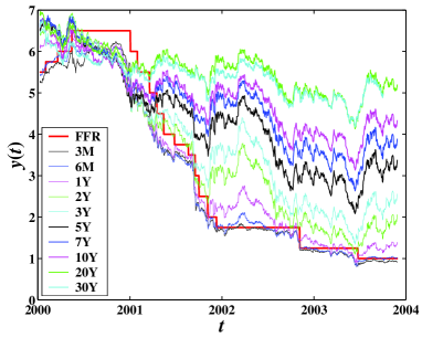
Figure 1: (Color online) Time evolution of ten yields with the maturities 3M (three months), 6M, 1Y (one year), 2Y, 3Y, 5Y, 7Y, 10Y, 20Y, 30Y and of the Federal funds rate since January 2000.

Figure 2 and Table 1 show the results of the fits of the ten yields with different maturities (3M, 6M, 1Y, 2Y, 3Y, 5Y, 7Y, 10Y, 20Y, 30Y) shown in Fig. 1 with the first-order ($N=1$) LPPL formula (1). The yields with maturities no less than 2Y are similar to each other with approximately synchronous log-periodic oscillations. Yields with short maturities (3M, 6M, and 1Y) exhibit different shapes. The parameters of the fits of (1) with $N=1$ to the yields are listed in Table 1.

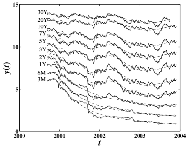
Figure 2: Time series (wiggly lines) of the yields with ten different maturities (3M, 6M, 1Y, 2Y, 3Y, 5Y, 7Y, 10Y, 20Y, 30Y) and their fits (dashed lines) using the first order ($N=1$) LPPL formula (1). The parameters of the fits are listed in Table 1. The yields with maturities greater than three months have been shifted vertically upwards by 0.9% incrementally.

Several interesting features can be extracted from this analysis. First of all, we observe a universal log-periodic oscillatory structure for yields with maturities no less than 2Y, with approximately the same angular log-frequencies $\omega\approx 7.4$, as given in Table 1. In contrast, for the yields with maturities 3M, 6M and 1Y, the small values of $\omega$ and the values of the exponents $m$ close to $1$ (absence of curvature) or to $0$ (curvature localized close to $t_{c}$) indicate the absence of LPPL.

Table 1: Parameters of the fits with the first-order LPPL formula (1) with $N=1$ off the ten U.S. Treasury bond yields shown in Fig. 1.

Maturity	$t_{c}$	$m$	$\omega$	$\phi_{1}$	$A$	$B$	$C_{1}$	$\chi$
3M	2000/10/22	1.00	1.40	4.13	6.186	-0.00823	0.00408	0.206
6M	2000/10/19	0.98	1.29	3.42	6.132	-0.00884	0.00454	0.199
1Y	2000/10/15	0.15	0.85	2.80	8.411	-1.97804	0.55760	0.230
2Y	2000/10/08	0.42	7.94	6.23	6.855	-0.28056	0.02946	0.224
3Y	2000/10/07	0.49	7.73	4.84	6.366	-0.14033	0.02216	0.249
5Y	2000/10/01	0.64	7.60	4.01	5.883	-0.03523	0.00861	0.262
7Y	2000/09/29	0.67	7.43	2.95	5.889	-0.02138	0.00639	0.247
10Y	2000/10/21	0.64	7.06	0.26	5.730	-0.01959	0.00805	0.236
20Y	2000/10/19	0.75	6.87	5.40	5.965	-0.00452	0.00295	0.205
30Y	2000/09/28	0.80	7.52	3.61	5.775	-0.00289	0.00179	0.187

Secondly, the estimated inception dates $t_{c}$ for the yield antibubbles are consistent across all maturities to within three weeks, approximately in the first half of October 2000. This places the inception of the yield antibubble about two months after that of the worldwide antibubble (first half of August 2000) [1, 2, 4, 5]. In spite of the absence of a well-developed log-periodic structure for the 3-month yield, the power law still provides a reasonable estimation of $t_{c}$.

Thirdly, the progressive return of the yield curve to its normal upward concave shape after October 2000 is reflected in the decrease of the absolute value of the coefficient $B$ with maturity: a larger $|B|$ for the smaller maturities imply that the corresponding yields are decaying faster as a function of time. This leads to a growing spread and quantifies the evolution of the yield curve from a basically flat shape in October 2000 to a normal upward concave shape later. We find that the coefficient $|B|$ for a given yield maturity $\theta$ is approximately inversely proportional to the inverse of the square of the maturity:

$$|B|\sim{1\over\theta^{2}}~{}.$$ (2)

This dependence is different from that derived from the square-root law proposed in [13, 14, 15] to describe the normal regime, based on a Value-at-Risk like pricing of the forward rate curve. This is an additional evidence suggesting that the antibubble corresponds to an anomalous (or at least different) regime.

2.2 Statistical significance of the log-periodic structure

To assess the significance level of the observed log-periodic pattern, we present several statistical tests based on spectral analysis. The standard test consists in performing a Lomb periodogram analysis of the de-trended time series

$$S(\ln(t))=\frac{y(t)-A}{(t-t_{c})^{m}}~{},$$ (3)

in the manner introduced in Ref. [36] in a similar context. The Lomb periodogram analysis is analogous to a Fourier transform but for unevenly spaced data [37]. If $y(t)$ possesses log-periodic power law structure, $S$ has regular cosine undulations in the variable $\ln(t)$. Figure 3 shows the ten Lomb periodograms of the detrended signal of the ten treasury security yields. Except for the 3M and 6M yields, all the other eight yields exhibit a significant Lomb peak at the same fundamental angular log-frequency $\omega$ and also present peaks at harmonics $n\omega$ (where $n$ is an integer). It is interesting to observe that the parametric fit of the 1Y yield with formula (1) fails to qualify a LPPL structure while the present non-parametric method unearths a clear log-periodic structure. The two highest peaks are found for the maturities 2Y and 3Y. The thickest line shows the average of the Lomb periodograms over the eight periodograms of the yields with maturities larger than 6M. This averaging procedure has been introduced in [38] as an efficient way of enhancing a periodic or log-periodic signal when one has the luxury of an ensemble of realizations. Our present average amounts to postulate that each of the eight maturities larger than 6M has the same log-periodicity but with different residual noises.

The average normalized Lomb periodogram has its highest peak equal to $P_{N}(\omega_{f})=121$ at the fundamental angular log-frequency $\omega_{f}=7.92$. The false-alarm probability under the null hypothesis of i.i.d. Gaussian fit residuals is zero [37]. But assuming an i.i.d. structure is too restrictive (too optimistic) as the fit residuals have a dependence. We assume that this dependence can be approximated by the model of fractional Brownian noise with a Hurst exponent $H>1/2$. We can use our previous construction of a table of false alarm probabilities for various values of $H$ [39]. For $H=0.6$, the false alarm probability corresponding to the observed peak $P_{N}(\omega_{f})=121$ is $<0.01\%$, for $H=0.7$ it is $0.2\%$, for $H=0.8$ it is $3\%$ and for $H=0.9$ it is $20\%$. This means that the statistical significance of the log-periodicity is very high.

Bothmer has addressed the problem of the influence of noise dependence in the determination of the statistical significance of log-periodic oscillations [40]. He considers specifically the dependence introduced in data which have a cumulative nature (like a price which is the logarithm of the sum of returns). For this, Bothmer introduced the so-called cumulative Lomb periodogram and found it to be exponentially distributed independently of the frequency [40] for the null hypothesis of no oscillations. Actually, using a data set which involves a sum of noise contributions around a power law leads to a spurious peak on the Lomb periodogram corresponding to a most probable noise [41]. This mechanism explains the peak at $\omega_{\rm{mp}}=2.42$ observed in the averaged Lomb periodogram, which corresponds to about $1-1.5$ oscillations over the whole time span.

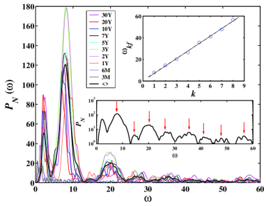
Figure 3: (Color online) Lomb periodograms of the detrended residuals of the ten treasury security yields and their Lomb average shown as the thickest line (referd to in the legend as “$\langle\rangle$”). Except for the 3M and 6M yields, all the other eight yield residues exhibit a significant Lomb peak at approximately the same fundamental angular log-frequency on on several of its harmonics. The lower inset shows the averaged Lomb periodogram in semi-log plot. The vertical arrows point to the peaks that identify a series of characteristic angular log-frequencies $\omega_{kf}$’s used to construct the upper inset. The upper inset presents the relation between $\omega_{kf}$ and $k$ for $k=1,2,\cdots,8$. The solid line shows an unconstrained linear regression, while the dashed line is the linear regression with the constraint of passing through the origin.

A strong additional evidence for log-periodicity lies on the presence of several higher-order harmonics of the fundamental $\omega_{f}$, as illustrated in the lower inset of Fig. 3. Here, we follow our previous aproach applied to hydrodynamic turbulence [42, 43]. The vertical arrows point to the peaks that identify a series of characteristic angular log-frequencies $\omega_{kf}$’s as a function of their order $k$ from left to right. The upper inset of Fig. 3 shows the linear relationship between the $\omega_{kf}$’s as a function of their order $k$ for $k=1,2,\cdots,8$. A linear regression is shown as the dashed line and gives $\omega_{kf}=6.87k+0.35$. The value $6.87$ slightly under-estimates the previously determined fundamental frequency $\omega_{f}=7.04$, and results from the positive intercept $0.35$. If we interpret the $\omega_{kf}$’s as the harmonics of $\omega_{f}$, we should expect $\omega_{kf}=k\omega_{f}$. The solid line of the upper inset of Fig. 3 shows the corresponding linear regression with the constraint of passing through the origin. This gives the relation $\omega_{f}=6.93$, which is in good agreement with our previous determination $\omega_{f}=7.04$. Another straightforward method is to form the ratios $\omega_{kf}/k$, which should be constant and equal to $\omega_{f}$ if the $\omega_{kf}$ are indeed the harmonics of $\omega_{f}$. We find $\langle{\omega_{kf}/k}\rangle=7.05\pm 0.42$, again confirming the value of the fundamental angular log-frequency and the presence of several harmonics.

Let us end this section by a note of caution. We have termed “non-parametric” the Lomb analysis of the residues defined by (3). Strictly speaking, this is not entirely correct, since the construction of $S$ uses the fitted $t_{c}$, $m$, and $A$ parameters, as criticized by [44]. This problem can be alleviated in several ways. One solution is to fit the data first using a pure power law, setting $C_{1}=0$ in Eq. (1), to obtain $A$, $m$ and $t_{c}$. Then, the parameters do not contain information on the searched log-periodicity (at the linear level of description). We have made these tests and find no differences in the results. An alternative solution is to estimate $A$ and $t_{c}$ by maximizing the linear correlation coefficient betwen $\ln(t-t_{c})$ and $y(t)-A$ and then obtain $m$ with a simple linear regression of the two aforementioned sequences [40]. In addition, one can also perform a generalized $q$-analysis on the data $y(t)$ by scanning $t_{c}$ [45]. This last method has been applied to test log-periodicity in stock market bubbles and antibubbles [1, 46], in the USA foreign capital inflow bubble ending in early 2001 [47], and in the ongoing UK real estate bubble [48]. We shall use it in section 5 to analyze the log-periodic patterns of the Federal funds rate.

3 The third-order harmonic

Previous analyses have shown that higher-order harmonics provide significant contributions to the structure of antibubbles [1, 2, 5]. The antibubble documented here on the yields is no exception as we now document. Figure 3 and in particular its lower inset shows that the leading contribution to the power spectrum is provided by the third harmonics $\omega_{3f}=3\omega_{f}$ rather than by the second one $\omega_{2f}=2\omega_{f}$. This is reminiscent of the log-periodicity found in two-dimensional hydrodynamic turbulence where the strongest harmonics is also for $3\omega_{f}$ while $2\omega_{f}$ gives almost no contribution [49]. This suggests that, in the spirit of a Landau expansion of the type used in [50, 51], the nonlinearity is third-order rather than quadratic.

To test quantitatively the impact of the third harmonic, we thus extend the previous parametric fit in section 2.1 by using expression (1) with $N=3$ but fixing the coefficient $C_{2}=0$ of the second harmonic. Figure 4 shows the corresponding ten fits of the ten yields, whose parameters are listed in Table 2. Again, the fits to the yields with maturity larger than two years exhibit evident LPPL signatures. The corresponding values of $t_{c}$, $m$ and $\omega$ of these six fits are close to those obtained with the simple first-order LPPL fits. These results are consistent with the spectral analysis reported in Fig. 3. Since the power calculated in the Lomb periodogram is proportional to the square of the amplitude of the periodic component, for this parametric analysis to be consistent with the non-parametric power spectrum, we should have

$$\frac{P_{N}(\omega_{f})}{P_{N}(\omega_{nf})}=\left(\frac{C_{1}}{C_{n}}\right)^{2}.$$ (4)

From Fig. 3, we measure ${P_{N}(\omega_{f})}/{P_{N}(\omega_{3f})}=5.8$ for the averaged Lomb periodogram. On the other hand, $\left({C_{1}}/{C_{3}}\right)^{2}$ is in the range $5-10$ for the five yields with larger maturities, using the values reported in Table 2. This is in reasonable agreement with (4). A similar consistency has been reported previously for the US 2000 S&P 500 antibubble [1].

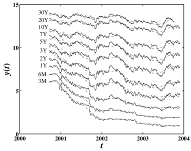
Figure 4: Time evolution (wiggly lines) of the Yields with ten different maturities (3M, 6M, 1Y, 2Y, 3Y, 5Y, 7Y, 10Y, 20Y, 30Y) and their fits using formula (1) with $N=3$ and $C_{2}=0$, taking into account the third-order harmonic component. The parameters of the fits are listed in Table 2. The yields with maturities greater than three months (3M) have been shifted vertically upwards by 0.9% incrementally for clarity.

Table 2: Parameters of fits to the ten yields shown in Fig. 4 using the LPPL formula (1) with $N=3$ and $C_{2}=0$.

Mat	$t_{c}$	$m$	$\omega$	$\phi_{1}$	$\phi_{3}$	$A$	$B$	$C_{1}$	$C_{3}$	$\chi^{\prime}$
3M	1999/12/08	0.04	4.35	0.35	1.48	100.9	-77.25	0.4760	0.1817	0.139
6M	1999/12/19	-0.06	4.30	6.24	0.17	-56.32	85.93	0.7242	0.3329	0.132
1Y	2000/01/20	-0.08	4.15	4.82	2.39	-35.84	65.38	0.5120	0.4529	0.163
2Y	2000/04/15	0.26	3.51	5.44	0.48	13.19	-1.946	0.0359	0.0795	0.219
3Y	2000/10/07	0.48	7.31	3.09	2.06	6.38	-0.1542	0.0241	0.0044	0.244
5Y	2000/10/09	0.63	7.00	0.01	2.44	5.83	-0.0368	0.0089	0.0028	0.246
7Y	2000/10/24	0.66	6.80	4.84	4.20	5.81	-0.0230	0.0070	0.0022	0.227
10Y	2000/10/25	0.64	6.79	4.74	3.98	5.71	-0.0190	0.0074	0.0025	0.215
20Y	2000/10/23	0.74	6.73	4.47	2.87	5.98	-0.0052	0.0030	0.0012	0.183
30Y	2000/10/30	0.77	6.70	4.13	2.30	5.74	-0.0034	0.0023	0.0010	0.168

Table 2 shows some systematic effects in the variations of the parameters $t_{c}$, $m$ and $\omega$ as a function of maturity, for the six yields with maturity larger than two years. Firstly, the estimated critical time $t_{c}$ increases slightly but systematically, suggesting an increasing (small) lag of the antibubble inception with increasing maturity. Secondly, the exponent $m$ increases with maturity. Thirdly, the angular log-frequency $\omega$ decreases. We will come back to these observations to propose an interpretation.

Is the inclusion of the third-order log-periodic component significant? Comparing Table 1 with Table 2, we observe that the fits including the third-order term lead to a $\sim 10\%$ reduction in the r.m.s. of the residuals. The fact that there is an improvement is not surprising since there are more parameters. However, since the third-order formula (1) with $N=3$ contains the first-order formula (1) with $N=1$ as a special case, we can use the statistics of embedded hypothesis and the Wilks test [53] to check if the hypothesis $C_{3}=0$ can be rejected. Under the hypothesis of i.i.d. normal residuals, the probability for $C_{3}=0$ to be rejected is equal to the probability that a variable taken from a chi-square distribution with 2 degrees of freedom (two is the difference in the number of parameters between the two formulas with $N=3$ and $N=1$ with $C_{2}=0$) exceeds $2n\ln(\chi/\chi^{\prime})$, where $n$ is the size of the time series. For the six yields with maturities larger than 2 years, we have $2n\ln(\chi/\chi^{\prime})=$ 30, 99, 131, 146, 170, and 166, respectively. This gives a probability that $C_{3}=0$ of less than $0.01\%$. Therefore, the third-order log-periodic component appears to be very significant.

4 A hierarchy of antibubbles

The theory underlying the LPPL formula (1) uses a so-called renormalization group formalism, which suggests that the large scale LPPL structure studied until now may cascade down the scales, such that LPPL structures can be observed at many different scales [52, 35, 2]. Such a hierarchical structure with LPPL observed as several embedded scales has been noticed over the years by several investigators (private communications) but was first mentioned in print at a qualitative level in a discussion of the Deutsche Aktien Index (German stock index) bubble before its burst in 1998 [54]. There has not been a convincing demonstration however that the LPPL patterns can be observed unambiguously at different time scales because small-scale structures are vulnerable to noise [4]. The observation of LPPL at several embedded scales become feasible when the large scale is very large, so that the smaller scales remain large. This situation describes the Japanese Nikkei 225 index: an antibubble was identified quantitatively to start in 2000, that is, on top of the more-than-one-decade long antibubble since 1990 [5]. In this case, the small LPPL structure spans more than one year. Actually, one year (or maybe down to six months) might be the lower cutoff for the detection of statistically significant LPPL structures in financial bubbles or antibubbles, based on daily data. Johansen proposed that LPPL patterns can only be ascertained about a time scale of one or two years [3]. Here we provide yet another example of such LPPL-within-LPPL structure for the yield data.

Figure 5 shows 29 years of the evolution of the U.S. 10-year treasury bond yield from 1975 to 2003. It is interesting to realize that the evolution at such large time scales can be represented also by an antibubble that started in 1979. The inception of this antibubble of the yield is associated with the peak in 1979-1980 of the inflation rate. Figure 5 also shows three small-scale antibubbles embedded within the large-scale. We have fitted these four antibubbles with the first-order LPPL formula (1). The data set used in these fits goes from the local high to the local low that breaks the structure when available [55]. The smooth oscillatory lines in Fig. 5 show the fits to a large-scale antibubble and three small-scale antibubbles.

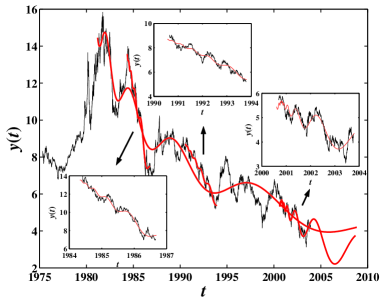
Figure 5: Illustration of the concept of a hierarchy of LPPL structures in antibubbles. The figure shows a large-scale antibubble on the U.S. 10-year treasury bond yield from 1979 to 2003. In addition , three small-scale antibubbles are detected as shown in the insets which magnify the three small-scale antibubbles. The smooth oscillatory lines show the fits to a large-scale antibubble and three small-scale antibubbles.

The parameters of the four fits are the following. The data set of the large-scale antibubble used in the LPPL fit is from 1981/09/30 to 2003/10/03 and we find $t_{c}={\rm{1979/01/04}}$, $m=-0.17$, $\omega=10.36$, $\phi=0.52$, $A=-15.27$, $B=98.5917$, $C=-3.4737$, with a r.m.s. of the fit residuals equal to $\chi=0.711$. The data set for the first small-scale antibubble used in the LPPL fit goes from 1984/05/30 to 1986/08/29 and we find $t_{c}={\rm{1984/02/23}}$, $m=1.04$, $\omega=12.41$, $\phi=4.20$, $A=14.01$, $B=-0.0057$, $C=0.0006$, with a r.m.s. of the fit residuals equal to $\chi=0.323$. The data set of the second small-scale antibubble goes from 1990/08/24 to 1993/10/15 and we find $t_{c}={\rm{1989/10/28}}$, $m=0.99$, $\omega=11.19$, $\phi=2.10$, $A=9.49$, $B=-0.0027$, $C=0.0002$, with the r.m.s. of the fit residuals equal to $\chi=0.233$. The data set of the third small-scale antibubble goes from 2000/09/09 to 2003/10/10 and we find $t_{c}={\rm{2000/10/23}}$, $m=0.62$, $\omega=7.03$, $\phi=3.18$, $A=5.72$, $B=-0.0213$, $C=-0.0089$, with a r.m.s. of the fit residuals equal to $\chi=0.237$. This last antibubble has already been documented in Table 1.

The 1979-2003 large-scale antibubble and the recent 2000-2003 small-scale antibubble provide predictions for the future evolution of the 10-year yield, obtained by extrapolating the LPPL fits to the coming years. The extrapolation of the large-scale antibubble suggests that the 10-year yield will decrease for about two years and then rebound, while that of the small-scale antibubble suggests an increase following by a reversal during the first quarter of 2004 which could last two years before reverting to growing again. At face value, it seems that these two predictions are contradictory: they can not be both right. This is actually not the case: the essence of the renormalization group formulation of antibubbles is that small structures can be carried by larger structures, in the way exemplified in Figs. 6 and 7. The small-scale structure is carried by the large-scale structure and provides details of the overall pattern delineated by the large scale structure. Thus, the two scenarios shown in Fig. 5 can be reconciled by not opposing them but by combining them and viewing them as two predictions of the same overall multi-scale process observed at two different time resolutions. Combining the prediction of these two time scales suggest that the 10-year yield will decrease at large scale with local rallies and falls until its recovery two years later.

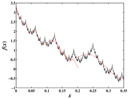
Figure 6: Weierstrass-Mandelbrot function [56, 57, 35] as a model of antibubbles within antibubbles within … The Weierstrass-Mandelbrot function is defined as $f(x)=\sum_{n=0}^{N}b^{n}\cos(a^{n}\pi x)$ with $N\to\infty$. The parameters used for this figure are $a=2$ and $b=1/2^{0}.5$. The two continuous lines show the fit of the Weierstrass-Mandelbrot function with equation (1) with $N=1$ both globally (large-scale antibubble) and locally (immediately smaller-scale antibubble). There are many more embedded smaller scales (actually an infinity when infinite resolution is available), corresponding to a self-similar fractal function.

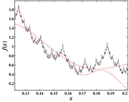
Figure 7: Magnification of Fig. 6.

5 Log-periodic patterns in Federal funds rate

It is well-known that the yields are driven by the Federal funds rate, which fixes the target overnight interest rate. The driving of the yields with longer maturities by the Federal funds rate is transmitted by the “rigidity” of the yield curve (or similarly of the forward rate curve) controlled by arbitraging [58, 59]. A simple picture is to imagine an elastic string whose handle (the Federal funds rate) is held by the Federal Reserve Chairman who moves it up or down, while the rest of the string slowly moves with lags and delays due to the interplay of inertial and elastic interactions.

In view of our finding of significant LPPL structures in yields with maturities larger than 2 years, the question naturally arises as to their origin. Are the LPPL structures intrinsic or endogenous to these yields with medium and large maturities? Or are they reflecting and amplifying a log-periodicity already present in the driving Federal funds rate? The difficulty of this question lies in the fact that the Federal funds rate is a staircase of plateaus with jumps and the number of jumps is not large. In a first bold attempt, we have fitted the Federal funds rate with the LPPL formula (1) following the same procedure used for fitting the other yields. We are not able to find a reliable signal because the power law part of the formula is absent. But, equation (1) contains two ingredients: (i) a power law $(t-t_{c})^{m}$ and a log-periodic oscillation $\cos[\omega\ln(t-t_{c})]$. Is it still possible for the log-periodic pattern to be present while the power law is absent? To address this question, we note that this amounts to asking if the times $t_{n}$ at which the funds rate is changed by the Federal Reserve could exhibit a geometric time series in the variable $t_{n}-t_{c}$ with a suitable value of $t_{c}$.

To our knowledge, the most robust method to attack this question is to use the generalized $(H,q)$-analysis on the Federal funds rate $y(t)$. The $(H,q)$-analysis [45, 46] is a generalization of the $q$-analysis [60, 61], which is a natural tool for the description of discretely scale invariant fractals. The $(H,q)$-derivative of the function $y(\tau)$ is defined as

$$D_{q}^{H}y(\tau)\stackrel{{\scriptstyle\triangle}}{{=}}\frac{y(\tau)-y(q\tau)}{[(1-q)\tau]^{H}}~{},$$ (5)

where $\tau=t-t_{c}$ is the time to the critical value $t_{c}$. The special case $H=1$ recovers the normal $q$-derivative, which itself reduces to the normal derivative in the limit $q\to 1^{-}$. There is no loss of generality by constraining $q$ in the open interval $(0,1)$ [45]. The parameter $q$ tests for the log-periodic structure, while $H$ acts as a high-pass filter to remove the global trend in the time series ensuring that the resultant series is almost stationary. The introduction of $H$ allows us to analyze non-fractal signals which nevertheless contain log-periodic components.

In order to perform the $(H,q)$-analysis of the Federal funds rate $y(t)$, we need to choose a value for $t_{c}$. In this goal, we use the following guidelines. First, Table 2 shows that $t_{c}$ for the yields decreases when the maturity decreases. Extrapolating, this suggests that the $t_{c}$ for the Federal funds rates is prior (but probably not much) to those estimated for the yields with larger maturities. This should be the case if the main driver of the yield rates was fixed by commercial banks who react following the central bank. It turns out that the $(H,q)$-analysis is very robust with respect to misspecification of $t_{c}$: the absence of an accurate estimate of $t_{c}$ does not impact much on the extraction of log-periodic components if (1) $q$ is close to $1$ so that the analysis is performed at a finer resolution and (2) $H$ is negative so that the part of $(H,q)$-derivative far from the critical time $t_{c}$ pays a more importance role in the analysis. In practice, using positive $H$’s give a majority of the angular log-frequencies with very low values: this can be interpreted to be caused by the remaining global trend in the signal. Also, if we use small $q$’s, we find small and unstable angular log-frequencies.

In order to implement concretely the $(H,q)$-analysis, we use here $t_{c}={\rm{2000/10/20}}$, which is compatible with the above considerations. We scan a $21\times 16$ rectangular grid in the $(H,q)$ parameter plane, with $H=-1:0.1:1$ and $q=0.6:0.02:0.9$. For each pair of $(H,q)$, we calculate the $(H,q)$-derivative, on which we perform a Lomb periodogram analysis. We have found that most of the Lomb periodograms have a similar shape as shown in Fig. 3. The highest Lomb peak of the resultant periodogram allows us to identify an angular log-frequency $\omega$ with its height $P_{N}$, which are both functions of $H$ and $q$. Figure 8 shows the histogram of occurrences of $\omega$. Its inset gives the bivariate distribution of pairs $(\omega,P_{N})$. There are clear clusters. The cluster peaked at low $\omega$ close to 1.7 is produced by relatively large (usually positive) $H$’s and relatively small $q$’s. The part of the histogram for $\omega<8$ corresponds to $q<0.76$. For $q>0.76$ and negative $H$’s, we see a well-defined cluster at $\omega$ close to $8.3\pm 0.2$ (indicated by an arrow with $\omega_{f}$). We attribute this value to the fundamental $\omega_{f}$. We can also discern two harmonics at $\omega_{2f}\approx 15.7$ and $\omega_{3f}\approx 22.5$, indicated by arrows.

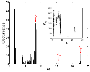
Figure 8: Histogram of the angular log-frequency $\omega$ of the most significant Lomb peaks in the generalized $(H,q)$-analysis of the Federal funds rate. The inset shows the bivariate distribution of the pairs $(\omega,P_{N})$ of the angular log-frequency at the largest peak of the Lomb periodograms, together with its amplitude $P_{N}$.

We thus conclude that there is no power law but a significant log-periodic structure in the Federal funds rate since October 2000, with an estimated angular log-frequency $\omega_{f}=8.3\pm 0.2$.

Theoretically, the $(H,q)$-analysis can be employed to estimate $t_{c}$ endogenously by searching for the highest Lomb peak obtained by varying $t_{c}$ in some range. However, the predictive power of this method has proven rather weak in other applications [45, 46] and we do not pursue it here. Changing $t_{c}$ by a few months both ways does not change significantly our conclusions.

6 Causality between stock markets and Federal funds rate

The similarity between the LPPL structures observed in the stock market since August 2000 and in the yields since October 2000 begs the question of the origin of these common properties. Let us consider the following scenarios.

1. Is the FRB (reacting to macroeconomic indicators together with its monetary policy) the source of log-periodicity in the timing of its interventions, which then spills over and is amplified in the yields with larger maturities, themselves influencing the stock market? In this scenario, the FRB is the source of log-periodicity in its response to other stimuli, which is then transferred to bonds and then to stocks.

2. Is the stock market first developing LPPL which then influence the yields of large maturities, both of them influencing the FRB timing of its intervention?

3. Or, keeping the hypothesis of the primary influence of the LPPL of the stock market, is the FRB the secondary step in reacting to the stock market which then spills over and influences the yields with larger maturities?

4. Is the LPPL observed both on the stock market and the yields the result of an overarching common origin to which they respond almost simultaneously?

In short, we address a problem of causality between two or more time series, which has a rich literature in economics (see for instance [62, 63] and references therein). Determining causality is notoriously difficult and often ill-defined and one has in general to assume drastic simplifications, such as stationarity of the time series, linear least-squares projections, and mean-square errors. While these assumptions are convenient to make when conducting empirical tests, they are not realistic. Here, we draw from our analysis to propose that the most probable scenario is number 2: Stock Market $\to$ Fed Reserve (Federal funds rate) $\to$ short-term yields $\to$ long-term yields. This conclusion is based on the following.

First, we have found that the critical inception times $t_{c}$ of the yields as well as of the Federal funds rate are about two months after that of the 2000 US stock market antibubble. In addition, $t_{c}$ tends to increase with the yield maturity.

Second, we notice that the log-periodic angular frequency decreases from the value $\omega=10.3\pm 0.2$ for the S&P 500 Index to $\omega=8.3\pm 0.2$ for the Federal funds rate and to values $7<\omega<8$ for yields when increasing their maturity (see Table 2). This trend in $\omega$ is consistent with the view that the Federal funds rate cuts was driven by the US stock market oscillations and thus developed a lower log-periodic frequency, which in turn drove the yields into still lower log-periodic frequencies.

Third, Fig. 9 shows in the same plot the Federal funds rate $y(t)$, the logarithm of the S&P 500 Index $x(t)$, and the logarithm of the NASDAQ Composite $z(t)$. One observes that the Federal funds rate $y(t)$ was increasing in the bull market and has been decreasing in bear market. After the burst of the new economy bubble, the Federal Reserve cut the interest rate from $6^{\frac{1}{2}}$ to 6 on 2001/01/03, at a time lagging more than four months behind the onset of the stock market antibubble and more than eight months after the burst of the bubble. This suggests that this Federal Reserve’s interest rate moves in the recent period have been caused at least partially by the behavior of the stock markets.

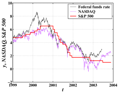
Figure 9: (Color online) Comparison of the Federal funds rate, the S&P 500 Index $x(t)$, and the NASDAQ Composite $z(t)$, from 1999 to mid-2003. To allow a illustrative visual comparison, the indices have been translated and scaled as follows: $x\to 5x-34$ and $z\to 10z-67$.

Fourth, Fig. 10 presents the cross-correlation between the Federal funds rate and the S&P 500 Index in the time period from October 1999 to mid-2003. The results are essentially the same when varying the start date from October 1999 to October 2000. Specifically, we construct the increments $\Delta y(t)$ of the Federal funds rate and of the logarithm of the S&P 500 Index (which defines the returns $\Delta\ln x(t)$) at the weekly, monthly and quarterly scales. Taking increments ensure to work with time series which are approximately stationary. We then calculate the cross-correlation coefficient with the Federal funds rate translated by $n$ time steps (trading days) according to the formula

$$C(n)={\rm{Corr}}\left(\Delta\ln x(t),\Delta y(t+n)\right)~{},$$ (6)

where ${\rm{Corr}}(x,y)$ is the statistical correlation between $x$ and $y$. Figure 10 shows the cross-correlation coefficient function $C(n)$ as a function of $n\in[-300,300]$ for the three time scales. While the weekly scale is too noisy to conclude, the cross-correlation coefficient exhibits a clear maximum for the two other time scales for a positive lag in the range 30-50 trading days: such a positive lag means that the S&P 500 Index in the past has a predictive power on the Federal funds rate in the future. Since correlations detect only linear predictability, this means that there is a linear (Granger) predictability of the Federal funds rate by the stock market.

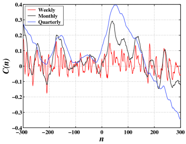
Figure 10: (Color online) Cross-correlation coefficient $C(n)$ between the increments of the logarithm of the S&P 500 Index and the increments of the Federal funds rate as a function of time lag $n$ in days. The three curves corresponds to three different time steps used to calculate the increments: weekly, monthly and quarterly. A positive lag $n$ corresponds to having the Federal funds rate posterior to the stock market.

Figure 11 is similar to Fig. 10 with the following modifications: it uses a single time scale of one quarter to calculate the increments and shows the cross-correlation coefficient between the increments of the logarithm of the S&P 500 Index and the increments of the lagged yields for all maturities 0M (Federal funds rate), 3M, 6M, 1Y, 2Y, 3Y, 5Y, 7Y, 10Y, 20Y and 30Y.

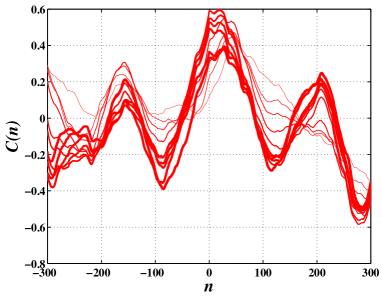
Figure 11: Each curve shows the cross-correlation coefficient $C(n)$ between the increments of the logarithm of the S&P 500 Index and the increments of the lagged bond yield at a given maturity as a function of time lag $n$. There are 11 curves with increasing line width corresponding to the maturities 0M (Federal funds rate), 3M, 6M, 1Y, 2Y, 3Y, 5Y, 7Y, 10Y, 20Y and 30Y. The increments have been calculated using a time scale of one month. A positive lag $n$ corresponds to having a bond yield posterior to the stock market.

Fig. 11 exhibits the robust feature that the cross-correlation coefficients of the pairs (stock market; bond yield) for the smallest maturities 0M (Federal funds rate), 3M, 6M, 1Y peak for a lag close to 30-50 days. In contrast, the yields with longer maturities have their cross-correlation with the S&P 500 Index exhibit two peaks, one for a lag around 30 days and one for a zero lag. This gives us an important information in addition to that obtained from Fig. 10: not only do we see the impact of the S&P 500 Index in the past on all future bond yields, we also find that the S&P 500 Index is impacting or causing the variation of the bond yield with large maturities instantaneously. This is consistent with the scenario in which the S&P 500 Index “causes” the FRB moves which itself drives the yields with the shorter maturities and at the same time the yields with the longer maturities are directly and instantaneously influenced by the S&P 500 Index (and the stock market more generally). In other words, we are uncovering the existence of two driving forces on the yields: the stock market and the monetary policy of the FRB. The stock market prevails strongly for long-term yields and in addition influences significantly causally the FRB actions which then dominates in its influence on the short-term yields.

The existence of a positive lag found here means that the S&P 500 Index in the past has a linear Granger predictive power on bond yields in the future for all maturities In other words, we can assert that there is a Granger causality of the stock market on the bond yields, at least in the recent past, from 2000 till mid-2003.

7 Conclusion

Using the descriptive method of log-periodic power laws (LPPL) based on a theory of behavioral herding, we have shown the existence of an antibubble in the yields of maturities larger than 1 year since October 2000. The concept of “antibubble” describes the existence of a specific LPPL pattern that is thought to reflect collective herding effects. We have presented a series of tests on the significance of log-periodicity: based on the existence of strong harmonics, on the fact that the dominant harmonics improve very significantly the power of explanation of the yield data, on the consistency between our parametric and non-parametric analyses, we can assert the existence of the LPPL antibubble on the yields since October 2000. We have then performed a simple cross-correlation calculation which has confirmed the following scenario, already suggested from the dependence of the parameters of the LPPL formula as a function of yield maturities:

• Herding and competition with value investing has led to a collective LPPL antibubble unfolding in the U.S. stock markets since August 2000 (and which may have already ended [64]).

• The Federal Reserve Board (FRB) reacted to and lagged (by about 30 trading days) behind the log-periodicity of the stock markets by a series of steps lowering the Federal funds rate according to a pattern mimicking the log-periodicity of the stock market.

• The yields with maturities less than 1 or 2 years then followed by amplifying the FRB steps by the interplay of risk and herding.

• The yields with larger maturity were also influenced directly and instantaneously by the stock market.

Our interpretation is that the FRB is “causally slaved” to the stock market, because the later is now more and more considered as a proxy for the present and future health of economy. The impact of the stock market both economically and psychologically is obvious from the large fraction of the US population actively invested and by the sheer size of the stock market capitalization that has grown significantly larger than the GDP.

The present work reinforces the picture in which anticipations and collective beliefs play growing roles in controlling and shaping the future evolution of not only the stock market but also the economy itself.

Acknowledgments

We are grateful to P.M. Thomas for attracting our attention to this problem. This work was supported by the James S. Mc Donnell Foundation 21st century scientist award/studying complex system.

References

- [1] D. Sornette and W.-X. Zhou, The US 2000-2002 Market Descent: How Much Longer and Deeper? Quantitative Finance 2 (2002) 468-481.
- [2] W.-X. Zhou and D. Sornette, Renormalization group analysis of the 2000-2002 antibubble in the US S&P 500 index: Explanation of the hierarchy of five crashes and prediction, Physica A 330 (2003) 584-604.
- [3] A. Johansen, An alternative view, Quantitative Finance 3 (2003) C6-C7.
- [4] D. Sornette and W.-X. Zhou, The US 2000-2003 market descent: clarifications, Quantitative Finance 3 (2003) C39-C41.
- [5] W.-X. Zhou and D. Sornette, Evidence of a worldwide stock market log-periodic antibubble since mid-2000, Physica A 330 (2003) 543-583.
- [6] D. Sornette and A. Johansen, Significance of log-periodic precursors to financial crashes, Quantitative Finance 1 (2001) 452-471.
- [7] D. Sornette, Why Stock Markets Crash (Critical Events in Complex Financial Systems), Princeton University Press, Princeton, NJ, 2003.
- [8] D. Sornette, Critical market crashes, Phys. Rep. 378 (2003) 1-98.
- [9] A. Johansen and D. Sornette, Endogenous versus Exogenous Crashes in Financial Markets, in press in “Contemporary Issues in International Finance” (Nova Science Publishers, 2004) (http://arXiv.org/abs/cond-mat/0210509)
- [10] D. Reifschneider, R. Tedlow and J. Williams, Aggregate disturbances, monetary policy and the macroeconomy: the FRB/US perspective, Federal Reserve Bulletin, LXXXV (1999) 1-19.
- [11] R. Rigobon and B. Sack, Measuring the reaction of monetary policy to the stock market, The Quarterly Journal of Economics 118 (2003) 639-669.
- [12] M.T. Bohl, P.L. Siklos and T. Werner, Do Central Banks React to the Stock Market? The Case of the Bundesbank, (July 2003). http://ssrn.com/abstract=459272.
- [13] J.-P. Bouchaud, N. Sagna, R. Cont, N. El-Karoui and M. Potters, Phenomenology of the interest rate curve, Applied Mathematical Finance 6 (1999) 209-232.
- [14] A. Matacz and J.-P. Bouchaud, Explaining the forward interest rate term structure, International Journal of Theoretical and Applied Finance 3 (2000) 381-389.
- [15] A. Matacz and J.-P. Bouchaud, An empirical investigation of the forward interest rate term structure, International Journal of Theoretical and Applied Finance 3 (2000) 703-729.
- [16] A. Estrella and F.S. Mishkin, The predictive power of the term structure of interest rates in Europe and the United States: Implications for the European Central Bank, Eur. Econo. Rev. 41 (1997) 1375-1401.
- [17] A. Estrella and F.S. Mishkin, Predicting US recessions: Financial variables as leading indicators, Rev. Econ. Stat. 80 (1998) 45-61.
- [18] D. Ivanova, K. Lahiri and F. Seitz, Interest rate spreads as predictors of German inflation and business cycles, Int. J. Forecasting 16 (2000) 39-58.
- [19] C.R. Birchenhall, D.R. Osborn and M. Sensier, Predicting UK business cycle regimes, Scot. J. Polit. Econ. 48 (2001) 179-195.
- [20] R. Ahrens, Predicting recessions with interest rate spreads: a multicountry regime-switching analysis, J. Int. Money Finance 21 (2002) 519-537.
- [21] A. Estrella, A.P. Rodrigues and S. Schich, How stable is the predictive power of the yield curve? Evidence from Germany and the United States, Rev. Econ. Stat. 85 (2003) 629-644.
- [22] J.D. Hamilton and D.H. Kim, A reexamination of the predictability of economic activity using the yield spread, J. Money Credit Bank 34 (2002) 340-360.
- [23] C. Hassapis, Financial variables and real activity in Canada, Can. J. Econ. 36 (2003) 421-442.
- [24] M.A. Thoma and J.A. Gray, Financial market variables do not predict real activity, Econ. Inq. 36 (1998) 522-539.
- [25] C.E. Weber, Financial market variables do not predict real activity: Further evidence, Econ. Inq. 40 (2002) 80-90.
- [26] M. Qi, Predicting US recessions with leading indicators via neural network models, Int. J. Forecasting 17 (2001) 383-401.
- [27] M. Camacho and G. Perez-Quiros, This is what the leading indicators lead, J. Appl. Econ. 17 (2002) 61-80.
- [28] C. Brooks and S. Tsolacos, Linkages between property asset returns and interest rates: evidence for the UK, Appl. Econ. 33 (2001) 711-719.
- [29] M. Chauvet and S. Potter, Predicting a recession: evidence from the yield curve in the presence of structural breaks, Econ. Lett. 77 (2002) 245-253.
- [30] G.L. Shoesmith, Predicting national and regional recessions using probit modeling and interest-rate spreads, J. Regional Sci. 43 (2003) 373-392.
- [31] E. Middleton, ‘Animal spirits’ and expectations in U.S. recession forecasting, preprint at http://arxiv.org/abs/nlin.AO/0108012.
- [32] B.M. Roehner, Identifying the bottom line after a stock market crash, Int. J. Mod. Phys. C 11 (2000) 91-100.
- [33] B.G. Resnick and G.L. Shoesmith, Using the yield curve to time the stock market, Finance Anal. J. 58 (2002) 82-90.
- [34] N.G. Fosback, Stock Market Logic, Dearborn Financial Publishing Inc, Chicago, Illinois, 1992.
- [35] Gluzman, S. and D. Sornette, Log-periodic route to fractal functions, Phys. Rev. E 65 (2002) 036142.
- [36] A. Johansen, O. Ledoit and D. Sornette, Crashes as critical points, International Journal of Theoretical and Applied Finance 3 (2000) 219-255.
- [37] W. Press, S. Teukolsky, W. Vetterling, B. Flannery, Numerical Recipes in FORTRAN: The Art of Scientific Computing, Cambridge University, Cambridge, 1996.
- [38] A. Johansen and D. Sornette, Evidence of discrete scale invariance by canonical averaging, Int. J. Mod. Phys. C 9 (1998) 433-447.
- [39] W.-X. Zhou and Didier Sornette, Statistical Significance of Periodicity and Log-Periodicity with Heavy-Tailed Correlated Noise, Int. J. Mod. Phys. C 13 (2002) 137-170.
- [40] H.-C.G.v. Bothmer, Significance of log-periodic signatures in cumulative noise, Quantitative Finance 3 (2003) 370-375.
- [41] Y. Huang, A. Johansen, M.W. Lee, H. Saleur and D. Sornette, Artifactual Log-Periodicity in Finite-Size Data: Relevance for Earthquake Aftershocks, J. Geophys. Res. 105 (2000) 25451-25471.
- [42] W.-X. Zhou and D. Sornette, Evidence of Intermittent Cascades from Discrete Hierarchical Dissipation in Turbulence, Physica D 165 (2002) 94-125.
- [43] W.-X. Zhou, D. Sornette and V.F. Pisarenko, New evidence of discrete scale invariance in the energy dissipation of three-dimensional turbulence: Correlation approach and direct spectral detection, Int. J. Mod. Phys. C 14 (2003) 459-470.
- [44] J.A. Feigenbaum, More on a statistical analysis of log-periodic precursors to financial crashes, Quantitative Finance 1 (2001) 527-532.
- [45] W.-X. Zhou and D. Sornette, Generalized -Analysis of Log-Periodicity: Applications to Critical Ruptures, Phys. Rev. E 66 (2002) 046111.
- [46] W.-X. Zhou and D. Sornette, Non-Parametric Analyses of Log-Periodic Precursors to Financial Crashes, in press in Int. J. Mod. Phys. C, preprint at cond-mat/0205531.
- [47] D. Sornette and W.-X. Zhou, Evidence of fueling of the 2000 new economy bubble by foreign capital inflow: Implications for the future of the US economy and its stock market, Physica A 332 (2004) 412-440.
- [48] W.-X. Zhou and D. Sornette, 2000-2003 Real Estate Bubble in the UK but not in the USA, Physica A 329 (2003) 249-263.
- [49] A. Johansen, D. Sornette and A.E. Hansen, Punctuated vortex coalescence and discrete scale invariance in two-dimensional turbulence, Physica D 138 (2000) 302-315.
- [50] D. Sornette and A. Johansen, Large financial crashes, Physica A 245 (1997) 411-422.
- [51] A. Johansen and D. Sornette, Financial “anti-bubbles”: log-periodicity in Gold and Nikkei collapses, Int. J. Mod. Phys. C 10 (1999) 563-575.
- [52] D. Sornette, Discrete scale invariance and complex dimensions, Physics Reports 297 (1998) 239-270.
- [53] C. Rao, Linear statistical Inference and Its Applications, Wiley, New York, 1965.
- [54] S. Drozdz, F. Ruf, J. Speth and M. WojcikM, Imprints of log-periodic self-similarity in the stock market, Eur. Phys. J. B 10 (1999) 589-593.
- [55] A. Johansen, D. Sornette and O. Ledoit, Predicting financial crashes using discrete scale invariance, Journal of Risk 1 (1999) 5-32.
- [56] A.N. Singh, The theory and construction of non-differentiable functions, in Squaring the circle and other monographs (Chelsea Publishing Company, 1953).
- [57] M. V. Berry and Z. V. Lewis, On the Weierstrass-Mandelbrot fractal function, Proc. Roy. Soc. A 370, 459-484 (1980).
- [58] D. Sornette, “String” formulation of the Dynamics of the Forward Interest Rate Curve, European Physical Journal B 3 (1998) 125-137.
- [59] P. Santa-Clara and D. Sornette, The dynamics of the forward interest rate curve with stochastic string shocks, The Review of Financial Studies 14 (2001) 149-185.
- [60] A. Erzan, Finite -differences and the discrete renormalization group, Phys. Lett. A 225 (1997) 235-238.
- [61] A. Erzan and J.P. Eckmann, -analysis of Fractal Sets, Phys. Rev. Lett. 87 (1997) 3245-3248.
- [62] C.W.J. Granger (Author), E. Ghysels (Editor), N.R. Swanson (Editor), M.W. Watson (Editor), P. Hammond (Editor) and A. Holly (Editor), Essays in Econometrics: Volume 2, Causality, Integration and Cointegration, and Long Memory : Collected Papers of C.W.J. Granger (Cambridge, Cambridge University Press, 2001).
- [63] J. Geweke, Inference and Causality in Economic Time Series Models, Handbook of Econometrics Volume 2, Chapter 19, Ed. by H.V. Griliches and M.D. Intriligator (North-Holland, Elsevier Science Publishers BV, 1984).
- [64] W.-X. Zhou and D. Sornette, Testing the Stability of the 2000-2003 US Stock Market “Antibubble”, submitted to the Journal of Forecasting (http://arXiv.org/abs/cond-mat/0310092).