Relaxation of the Bose-condensate oscillations in the mesoscopic system at T=0

Abstract

The general system is given of nonlinear equations describing dissipationless evolution of the oscillating Bose-condensate. The relaxation of transverse oscillations of the condensate in a trap of the cylindric symmetry is considered. The evolution occurs due to parametric resonance coupling the transverse mode with the longitudinal ones. The nonlinear rescattering in the subsystem of discrete longitudinal modes results in suppression of the return of energy, yielding dissipationless nonmonotonic relaxation of transverse oscillations in the condensate.

The discovery of Bose-condensation in ultracold gases has yielded a unique possibility for the study of evolution of the coherent properties in the macroscopic system isolated from environment. One of most interesting aspects here is connected with clarifying and analyzing the nature of the damping of coherent oscillations in the condensate. So far, the theoretical and experimental investigation of the problem has been connected, in fact, with consideration of the damping at finite temperatures (see detailed bibliography in 1 ). In this case the ensemble of normal excitations plays effectively a role of the interior thermostat. The interaction with thermal excitations results in damping the condensate oscillations with the transfer of energy into the subsystem of normal excitations.

A question about the internal mechanism of damping at $T=0$ represents a special interest in this problem. In the work of authors 2 the existence of such mechanism is shown on the example dealing with the damping of the radial coherent oscillations in the condensate with the cylindric symmetry in the transverse parabolic potential. It is found that the damping arises from a special parametric resonance resulting in the transfer of energy into the subsystem of longitudinal modes. The parametric resonance is due to oscillations of the sound velocity as a result of transverse oscillations of the condensate. It should be emphasized that the results obtained in 2 can be used only for describing the initial period of damping.

To describe the damping at the large times in the isolated system of finite sizes with the discrete system of energy levels, it is necessary to know additionally the temporal evolution in the subsystem of transverse modes and involve variation of the parametric resonance with reducing the amplitude of transverse oscillations. This aspect is a significant difference from the conventional picture of parametric resonance. The choice of geometry of the system is determined by the fact that, for an arbitrary variation of the frequency in a two-dimensional parabolic potential of the circular symmetry and arbitrary magnitudes of parameters, as is strictly found in 3 (also 4 ), two-dimensional oscillations do not damp.

Recently, Paris group 1 has published the results of the experimental study on the damping of transverse modes in the condensate as a whole (breathing mode, BM) in the elongated trap with the azimuthal symmetry for extremely low temperature of 40nK. At the small magnitude of the BM amplitude the authors observe the record slow damping. For larger magnitude of the initial BM amplitude, the picture changes drastically. After the fall within a limited time interval the reverse transfer of energy with the growth of the BM amplitude starts. The normal behavior of damping recovers only a noticeable time interval later.

The theoretical analysis with explanation of the anormal picture is given in 5 . It is found that the involvement of nonlinear coupling between longitudinal and transverse modes is essential. However, the relaxation of longitudinal excitations was considered phenomenologically in essence.

In fact, for the discrete energy spectrum inherent in the closed mesoscopic system, the irreversible damping does not appear. It can be spoken only about the nonstationary redistribution of energy in the subsystem of longitudinal modes.

In the present work we have obtained a full set of nonlinear equations describing the temporal evolution of the oscillating condensate in the lack of the irreversible channels of dissipation. Our starting point is the Gross-Pitaevskii equation. The condensate of the cylindrical symmetry is considered in a transverse parabolic potential with longitudinal size $2L\gg R$ where $R$ is the static radius of the condensate. The analysis of the solution demonstrates an essential dependence of the damping of radial oscillations upon the character of evolution of longitudinal modes. Redistribution of the energy transferred into this subsystem results in the chaotic nonstationary picture of filling the discrete levels and simultaneously in the significant reduction for the amplitudes of active longitudinal modes excited directly as a result of parametric resonance. This reduction is equivalent effectively to relaxation but occurs in the lack of real dissipation.

We will consider the dynamics of Bose-condensate in a rarified gas at $T=0$ within the framework of the nonlinear Gross-Pitaevskii equation for condensate wavefunction $\Psi$

$$i\hbar\frac{\partial\Psi\left(\vec{r},t\right)}{\partial t}=[-\frac{\hbar^{2}}{2m}\nabla^{2}+V\left(\vec{r}\right)]\Psi\left(\vec{r},t\right)\\ +U_{0}\Psi^{\ast}\left(\vec{r},t\right)\Psi^{2}\left(\vec{r},t\right).$$ (1)

Here $U_{0}=4\pi\hbar^{2}a/m$ is the vertex of the local interaction between particles and $a$ is the scattering length. The system is assumed to be closed and in the course of evolution the number of particles $N$ and total energy $E$ conserve. We restrict ourselves by the case of repulsion between particles ($a>0$). Let us represent the wavefunction in the form

$$\Psi\left(\vec{r},t\right)=\sqrt{n\left(\vec{r},t\right)}e^{i\Phi\left(\vec{r},t\right)}$$

The imaginary part of Eq. (1) yields directly the equation of continuity for the condensate

$$\frac{\partial n_{1}\left(\vec{r},t\right)}{\partial t}+\nabla[(n_{0}\left(\vec{r}\right)+n_{1}\left(\vec{r},t\right)]\vec{v}\left(\vec{r},t\right) =0,$$ (2)

$$\vec{v}\left(\vec{r},t\right) =\frac{\hbar}{m}\nabla\Phi\left(\vec{r},t\right).$$

In (2) we introduced the fraction of density $n_{1}\left(\vec{r},t\right)$ depending explicitly on the time and represented the total density as $n\left(\vec{r},t\right)=n_{0}\left(\vec{r}\right)+n_{1}\left(\vec{r},t\right)$.

The real part of Eq. (1) yields an equation for the phase

$$-\hbar\frac{\partial\Phi}{\partial t}=\frac{\hbar^{2}}{2m}(\nabla\Phi)^{2}+U_{0}n+V\left(\vec{r}\right)-\frac{\hbar^{2}}{2m\sqrt{n}}\nabla^{2}\sqrt{n}.$$ (3)

Below we consider a gas of the sufficiently high density so that the correlation length $\xi=1/\sqrt{mn_{0}U_{0}}$ is small compared with all sizes of the system. It proves to be that only the long wave condensate excitations with the wavelengths larger than $\xi$ are involved into the processes considered. In these conditions corresponding to the Thomas-Fermi approximation the last term in (3) can be neglected, e.g., 6 . For the stationary case when $\vec{v}=0$, the phase of the condensate wavefunction has the familiar value $\Phi_{0}=-\mu_{0}t/\hbar$ where $\mu_{0}$ is the chemical potential. Then from equation (3) one has

$$n_{0}(\vec{r})=\frac{1}{U_{0}}\left(\mu_{0}-V(\vec{r})\right)$$ (4)

Keeping notation $\Phi$ for the phase connected with the condensate dynamics, we find

$$-\hbar\frac{\partial\Phi}{\partial t}=\frac{\hbar^{2}}{2m}(\nabla\Phi)^{2}+U_{0}n_{1}$$ (5)

A set of nonlinear equations (2) and (5) describes not only excitations of quantum fluid but also their interaction. We will strictly take this interaction into account, not involving the perturbation theory. Note that the external potential enters equations (2) and (5) only implicitly via the static distribution of density (4).

Within the linear approximation the system of equations (2) and (5) reduces to the equation of harmonic oscillations

$$\frac{\partial^{2}n_{1}}{\partial t^{2}}=c_{0}^{2}\nabla\left(f_{0}\nabla n_{1}\right).$$

Here

$$f_{0}(\vec{r})=\frac{n_{0}(\vec{r})}{n_{00}},\ n_{00}=n_{0}(0),\ c_{0}^{2}=\frac{U_{0}n_{00}}{m}=\frac{\mu_{0}}{m}.$$ (6)

Let us introduce the whole orthonormalized system of eigenfuctions of the harmonic problem $\left\{\chi_{s}(\vec{r})\right\}$ being solution of the equation

$$\Omega_{k}^{2}\chi_{s}(\vec{r})+c_{0}^{2}\nabla\left(f_{0}(\vec{r})\nabla\chi_{s}(\vec{r})\right)=0.$$ (7)

Let us expand $n_{1}$ and $\Phi$ in the whole system of eigenfunctions $\chi_{s}(\vec{r})$

$$n_{1}(t,\vec{r})={\displaystyle\sum\limits_{s}}c_{s}(t)\chi_{s}(\vec{r}),\ \ \ \Phi={\displaystyle\sum\limits_{s}}a_{s}(t)\chi_{s}(\vec{r})$$ (8)

Inserting these expansions into Eqs. (2) and (5), one finds

$$\begin{array}[c]{c}\frac{\partial}{\partial t}c_{s}-\frac{\hbar\Omega_{s}^{2}}{U_{0}}a_{s}=\frac{\hbar}{m}{\displaystyle\sum\limits_{s_{1}s_{2}}}c_{s_{1}}a_{s_{2}}\left\langle\chi_{s_{1}}\left(\nabla\chi_{s}^{\ast}\right)\left(\nabla\chi_{s_{2}}\right)\right\rangle\\ \frac{\partial}{\partial t}a_{p}+\frac{U_{0}}{\hbar}c_{p}=-\frac{\hbar}{2m}{\displaystyle\sum\limits_{s_{1}s_{2}}}a_{s_{1}}a_{s_{2}}\left\langle\chi_{s}^{\ast}\left(\nabla\chi_{s_{1}}\right)\left(\nabla\chi_{s_{2}}\right)\right\rangle\end{array}$$ (9)

Here $\left\langle...\right\rangle=\int d^{3}r(...)$. For the right-hand side of the first equation, we employ the transformation

$$\left\langle\chi_{s}^{\ast}\nabla(\chi_{s_{1}}\left(\nabla\chi_{s_{2}}\right))\right\rangle=-\left\langle\chi_{s_{1}}\left(\nabla\chi_{s}^{\ast}\right)\left(\nabla\chi_{s_{2}}\right)\right\rangle$$

Let us introduce new variables

$$a_{s}=\left(\frac{U_{0}}{\hbar\Omega_{s}}\right)^{1/2}(y_{s}+y_{-s}^{\ast}),\ \ \ c_{s}=i\left(\frac{\hbar\Omega_{s}}{U_{0}}\right)^{1/2}(y_{s}-y_{-s}^{\ast})$$

For the modes described by real eigenfunctions $\chi_{s}$, coefficients $a_{s}$, $b_{s}$ are real and $y_{-s}\equiv y_{s}$.

For these variables, Eqs. (9) can be represented as

$$\frac{\partial}{\partial t}y_{s}+i\Omega_{s}y_{s}={\displaystyle\sum\limits_{s_{1}s_{2}}}M_{ss_{1}s_{2}}(y_{s_{1}}-y_{-s_{1}}^{\ast})(y_{s_{2}}+y_{-s_{2}}^{\ast})\\ -\frac{1}{2}{\displaystyle\sum\limits_{s_{1}s_{2}}}K_{ss_{1}s_{2}}(y_{s_{1}}+y_{-s_{1}}^{\ast})(y_{s_{2}}+y_{-s_{2}}^{\ast})$$ (10)

Here

$$\begin{array}[c]{c}M_{ss_{1}s_{2}}=\frac{1}{2m}\left(\frac{\hbar U_{0}\Omega_{s_{1}}}{\Omega_{s}\Omega_{s_{2}}}\right)^{1/2}\left\langle\left(\nabla\chi_{s}^{\ast}\right)\chi_{s_{1}}\left(\nabla\chi_{s_{2}}\right)\right\rangle,\\ K_{ss_{1}s_{2}}=\frac{1}{2m}\left(\frac{\hbar U_{0}\Omega_{s}}{\Omega_{s_{1}}\Omega_{s_{2}}}\right)^{1/2}\left\langle\chi_{s}^{\ast}\left(\nabla\chi_{s_{1}}\right)\left(\nabla\chi_{s_{2}}\right)\right\rangle.\end{array}$$ (11)

Let at the initial time moment a transverse condensate oscillation alone be excited as a whole with conservation of the cylindrical symmetry (”breathing mode” and hereafter index $\perp$). A set of equations (10) can be represented in this case as

$$\begin{array}[c]{c}\frac{\partial}{\partial t}y_{\perp}+i\Omega_{\perp}y_{\perp}={\displaystyle\sum\limits_{k}}M_{\perp k-k}(y_{k}y_{-k}-y_{k}^{\ast}y_{-k}^{\ast})\\ -\frac{1}{2}{\displaystyle\sum\limits_{k}}K_{\perp k-k}(y_{k}+y_{-k}^{\ast})(y_{-k}+y_{k}^{\ast}),\\ \frac{\partial}{\partial t}y_{k}+i\Omega_{k}y_{k}=-2M_{kk\perp}y_{-k}^{\ast}(y_{\perp}+y_{\perp}^{\ast})\\ +K_{\perp k-k}(y_{\perp}-y_{\perp}^{\ast})(y_{k}+y_{-k}^{\ast})+I_{k}.\end{array}$$ (12)

In the second equation we use equalities $M_{k\perp k}=K_{\perp k-k},\ K_{kk\perp}=M_{kk\perp}$. The last term on the right-hand side determines the evolution in the longitudinal subsystem of excitations

$$I_{k}={\displaystyle\sum\limits_{k_{1}k_{2}}}M_{kk_{1}k_{2}}(y_{k_{1}}-y_{-k_{1}}^{\ast})(y_{k_{2}}+y_{-k_{2}}^{\ast})\\ -\frac{1}{2}{\displaystyle\sum\limits_{k_{1}k_{2}}}K_{kk_{1}k_{2}}(y_{k_{1}}+y_{-k_{1}}^{\ast})(y_{k_{2}}+y_{-k_{2}}^{\ast}).$$ (13)

The eigenfunction of the breathing mode is found from the solution of equation (7) involving that within the Thomas-Fermi approximation $f_{0}=1-r^{2}/R^{2}$ where $R^{2}=2c_{0}^{2}/\omega_{\perp}^{2}$, $\omega_{\perp}$ being the frequency of a parabolic trap.

$$\chi_{\perp}=\sqrt{\frac{3}{V}}(1-\frac{2r^{2}}{R^{2}}),\ \ \Omega_{\perp}=2\omega_{\perp},$$ (14)

Quantity $k$ determines the value of wave vector for longitudinal excitations, running discrete values due to finite sizes of the system in the $z$ direction. Following work 7 , it is easily to find the eigenfunctions and eigenvalues for the longwave longitudinal modes

$$\begin{array}[c]{c}\chi_{k}=\sqrt{\frac{1}{V}}e^{ikz}[1-\frac{\left(kR\right)^{2}}{16}(1-\frac{2r^{2}}{R^{2}})],\\ \Omega_{k}=\bar{c}k(1-\frac{\left(kR\right)^{2}}{96}),\ \bar{c}=\frac{c_{0}}{\sqrt{2}}.\end{array}$$ (15)

Using (14) and (15), one can straightforwardly calculate matrix elements (11) entering in (12)

$$\begin{array}[c]{c}M_{\perp k-k}=M_{kk\perp}=-\eta\frac{\sqrt{6}}{4}\left(\frac{\Omega_{k}}{\omega_{\perp}}\right)^{2},\\ K_{\perp k-k}=-\eta\frac{5\sqrt{6}}{24}\left(\frac{\Omega_{k}}{\omega_{\perp}}\right)^{3},\ \eta=\omega_{\perp}\left(\frac{\hbar\omega_{\perp}}{Vn_{00}\mu_{0}}\right)^{1/2}\end{array}$$ (16)

and in (13)

$$\begin{array}[c]{c}M_{kk_{1}k_{2}}=\eta\left(\frac{\Omega_{k}\Omega_{k_{1}}\Omega_{k_{2}}}{\omega_{\perp}^{3}}\right)^{1/2}\text{sign}(kk_{2})\delta_{k,k_{1}+k_{2}},\\ K_{kk_{1}k_{2}}=-\eta\left(\frac{\Omega_{k}\Omega_{k_{1}}\Omega_{k_{2}}}{\omega_{\perp}^{3}}\right)^{1/2}\text{sign}(k_{1}k_{2})\delta_{k,k_{1}+k_{2}}\end{array}$$ (17)

Equations (12) and (13) with matrix elements (16) and (17) describe fully the relaxation of the transverse condensate oscillations in the mesoscopic system in the lack of dissipative channels for evolution.

We assume that the initial amplitude of breathing mode is relatively small, i.e., $\left|\delta R/R\right|_{0}\ll 1$. This restricts a scale of the nonlinear interaction between modes. From the other side the energy interval in which the discrete longitudinal modes are connected effectively with the breathing mode proves to be small compared with $\omega_{\perp}$. Under conditions we can simplify a set of equations, restricting ourselves with the quasi resonance approximation. Within the framework of the approximation in equations (12) and (13) we can retain only the terms for which the following inequality is valid

$$\Delta\Omega=\left|\Omega_{s}\pm\Omega_{s_{1}}\pm\Omega_{s_{2}}\right|\ll\Omega_{s_{i}}$$ (18)

Let us rewrite equations (12) and (13) within this approximation, substituting ratios $\bar{y}_{s}=y_{s}(t)/\left|y_{\perp}(0)\right|$ for amplitudes $y_{s}$. The initial amplitude of breathing mode $y_{\perp}(0)$ can be found from comparing the vibrational energy of the condensate at the initial time moment $E_{vib}=\frac{4}{3}\mu_{0}N\left|\delta R/R\right|_{0}^{2}$ with the energy of transverse mode $2\hbar\Omega_{\perp}\left|y_{\perp}(0)\right|^{2}$. Hence

$$\left|y_{\perp}(0)\right|=\left(\frac{2\mu_{0}N}{3\hbar\Omega_{\perp}}\right)^{1/2}\left|\frac{\delta R}{R}\right|_{0}$$

After involvement of these notations equations (12) and (13) go over into

$$\frac{\partial}{\partial t}\bar{y}_{\perp}+i\Omega_{\perp}\bar{y}_{\perp}=-\alpha\underset{k>0}{\sum}^{\prime}\bar{y}_{k}\bar{y}_{-k},$$

A dash in a sum of the first equation means summation over ”active modes” alone, interacting directly with the BM according to restriction (18)

$$\frac{\partial}{\partial t}\bar{y}_{k}+i\Omega_{k}\bar{y}_{k}=\alpha\bar{y}_{-k}^{\ast}\bar{y}_{\perp}\\ +\alpha^{\prime}{\displaystyle\sum\limits_{k>k_{1}>0}}\left(\frac{\Omega_{k}\Omega_{k_{1}}\Omega_{k-k_{1}}}{\omega_{\perp}^{3}}\right)^{1/2}\bar{y}_{k_{1}}\bar{y}_{k-k_{1}}\\ -2\alpha^{\prime}{\displaystyle\sum\limits_{k_{1}>0}}\left(\frac{\Omega_{k}\Omega_{k_{1}}\Omega_{k+k_{1}}}{\omega_{\perp}^{3}}\right)^{1/2}\bar{y}_{k_{1}}^{\ast}\bar{y}_{k+k_{1}},\ \ (k>0)$$ (19)

For longitudinal modes which do not interact directly with the transverse mode, one should omit the first term on the right-hand side of Eq. (19). In these equations

$$\begin{array}[c]{l}\alpha=\left|\left(2M_{\perp k-k}-K_{\perp k-k}\right)\right|\left|y_{\perp}(0)\right|\approx 0,3\omega_{\perp}\left|\frac{\delta R}{R}\right|_{0},\\ \alpha^{\prime}\approx 2\alpha.\end{array}$$ (20)

Let us take that one has $\bar{y}_{k}(0)=\bar{y}_{-k}(0)$ for the trivially degenerated states at the initial time moment. It follows from a set of equations (19) that this equality holds in the course of evolution. To analyze, it is convenient to select the fast phase from complex variables $\bar{y}_{s}$, representing them as

$$\bar{y}_{s}=b_{s}\left(t\right)e^{-i(\Omega_{s}t+\varphi_{s}\left(t\right))},$$

where $b_{s}\left(t\right)$ and $\varphi_{s}\left(t\right)$ are the real quantities varying relatively slow in time at $\alpha/\omega_{\perp}\ll 1$. Let us introduce notations

$$\gamma_{kk_{1}k_{2}}=(\Omega_{k}-\Omega_{k_{1}}-\Omega_{k_{2}})t+(\varphi_{k}-\varphi_{k_{1}}-\varphi_{k_{2}})$$ (21)

Separating real and imaginary parts (19), one finds

$$\frac{\partial}{\partial t}b_{\perp}=-\alpha\underset{k>0}{\sum}^{\prime}b_{k}^{2}\cos\gamma_{\perp kk},\ \frac{\partial}{\partial t}\varphi_{\perp}=\alpha\underset{k>0}{\sum}^{\prime}\frac{b_{k}^{2}}{b_{\perp}}\sin\gamma_{\perp kk},$$ (22)

$$\begin{array}[c]{c}\frac{\partial}{\partial t}b_{k}=\alpha b_{k}b_{\perp}\cos\gamma_{\perp kk}+I_{k},\\ I_{k}=\alpha^{\prime}{\displaystyle\sum\limits_{k>k_{1}>0}}\left(\frac{\Omega_{k}\Omega_{k_{1}}\Omega_{k-k_{1}}}{\omega_{\perp}^{3}}\right)^{1/2}b_{k_{1}}b_{k-k_{1}}\cos\gamma_{kk_{1}k-k_{1}}\\ -2\alpha^{\prime}{\displaystyle\sum\limits_{k_{1}>0}}\left(\frac{\Omega_{k}\Omega_{k_{1}}\Omega_{k+k_{1}}}{\omega_{\perp}^{3}}\right)^{1/2}b_{k+k_{1}}b_{k_{1}}\cos\gamma_{k+k_{1}k_{1}k},\end{array}$$ (23)

$$\begin{array}[c]{c}\frac{\partial}{\partial t}\varphi_{k}=\alpha b_{\perp}\sin\gamma_{\perp kk}+I_{k}^{\prime},\\ I_{k}^{\prime}=-\alpha^{\prime}{\displaystyle\sum\limits_{k>k_{1}>0}}\left(\frac{\Omega_{k}\Omega_{k_{1}}\Omega_{k-k_{1}}}{\omega_{\perp}^{3}}\right)^{1/2}\frac{b_{k_{1}}b_{k-k_{1}}}{b_{k}}\sin\gamma_{kk_{1}k-k_{1}}\\ -2\alpha^{\prime}{\displaystyle\sum\limits_{k_{1}>0}}\left(\frac{\Omega_{k}\Omega_{k_{1}}\Omega_{k+k_{1}}}{\omega_{\perp}^{3}}\right)^{1/2}\frac{b_{k+k_{1}}b_{k_{1}}}{b_{k}}\sin\gamma_{k+k_{1}k_{1}k}.\end{array}$$ (24)

The analysis of the equations obtained allows us to find a scenario of relaxation of the transverse condensate oscillations. At the initial time moment the longitudinal modes are not excited and relation $b_{k}\left(0\right)\ll 1$ is valid for them, while according to definition $b_{\perp}\left(0\right)=1$. Thus at the initial time period the right-hand sides of Eq.  (22) and terms $I_{k}$, $I_{k}^{\prime}$ quadratic in $b_{k}$ play no role and evolution, in essence, is governed by first terms on the right-hand sides of equations (23) and (24) with constant $b_{\perp}$. The joint solution demonstrates an exponential growth $b_{k}(t)$ provided

$$\left|\Delta\Omega\right|\equiv\left|\Omega_{k}-\frac{1}{2}\Omega_{\perp}\right|<\alpha\,.$$ (25)

In particular, for $\left|\Delta\Omega\right|=0$, one has $\gamma_{\perp kk}\simeq 0$ and equation (23) yields $b_{k}(t)=b_{k}\left(0\right)\exp\alpha t$. These results, involving requirement of the finiteness for initial amplitude $b_{k}\left(0\right)$, are a typical manifestation of parametric resonance (cp. 2 ). All longitudinal modes within the energy interval of about $\alpha$ (active modes) experience an exponential growth. For the length of cylinder $2L$, the spacing between levels equals $\delta\Omega=\pi\bar{c}/L$. If $\delta\Omega<2\alpha$, at least, one mode lies within this interval. The growth of $b_{k}(t)$ results in reduction of $b_{\perp}(t)$ after some delay and transfer of energy to the other parallel modes at the same time. For $L\gg R$, there is a large number of such modes but a discrete character of energy spectrum results in the total prohibition of irreversible processes. However, irregular character of the transition amplitudes like $\left(\frac{\Omega_{k}\Omega_{k_{1}}\Omega_{k_{2}}}{\omega_{\perp}^{3}}\right)^{1/2}\cos\gamma_{kk_{1}k_{2}}$ in (23) and (24) in nonlinear terms $I_{k}$,$I_{k}^{\prime}$ leads to chaotic evolution in the system of longitudinal modes. One should think that in this case the return to the active longitudinal levels should significantly be suppressed and a noticeable fraction of the transferred energy should remain in inactive modes.

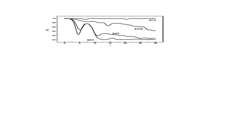
Figure 1: The behavior for the population of breathing mode as a function of the time at fixed value $k_{0}=10\pi/L$ for $\xi=0.5,\ 0.7,\ 0.95$, and $1.2$.

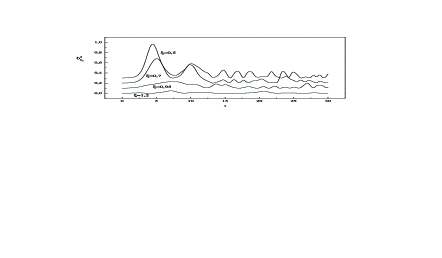
Figure 2: The behavior for the population of active mode $k_{0}$ as a function of the time at the same values $\xi$. The plots are shifted with respect to each other by $0.1$ along the vertical.

The direct numerical simulation of system (22)-(24) displays the picture described. Let only single level $k_{0}$ lie within the energy interval of about $\alpha$. We neglect weak dispersion of longitudinal modes (15). Then $\frac{\Omega_{k}\Omega_{k_{1}}\Omega_{k_{2}}}{\omega_{\perp}^{3}}\cong\frac{kk_{1}k_{2}}{k_{0}}$ and in expression (21) for longitudinal modes one can omit the first term. Let us introduce dimensionless time $\tau=\alpha t$ and take into account that $\alpha^{\prime}/\alpha=\text{const}$ (see, (20)). Then the evolution described depends, practically, on ratio $\xi=\Delta\Omega/\alpha$ alone and, to weak extent, on $k_{0}$ for $k_{0}L/\pi\gg 1$. (Note that this is valid not only in the quasi resonance approximation but also for the general system of equations (12).) In Fig.1 the dependence $b_{\perp}^{2}(\tau)$ $\equiv\left(\delta R(\tau)/\delta R(0)\right)^{2}$ is given at various magnitudes of parameter $\xi$ for fixed value $k_{0}$ (in units $\pi/L$). Here we involved not only the discrete levels lying below the active level but also the longitudinal levels above $k_{0}$ which start to be occupied at the next stage after decay of state $\pm k_{0}$. The law of energy conservation, which system (22)-(24) satisfies, results in a weak population of the upper levels in the course of evolution. In calculations we restricted ourselves by the same number of levels above and below $\Omega_{k_{0}}$. For value $\xi=1,\ 2$, the transverse oscillations does not decay at all. This is obviously seen from Fig.2 in which the behavior of population $b_{k_{0}}^{2}$ of level $k_{0}$ on $\tau$ is plotted for the same values of parameter $\xi$. For given value $\xi$, magnitude $b_{k_{0}}^{2}(\tau)$ remains close to zero for all $\tau$. The statement that the damping of oscillations at $T=0$ should be absent at all with violation of the conditions for appearance of parametric resonance (25) finds thus a direct confirmation. The curves corresponding to $\xi=0.7$ and $0.5$, on the contrary, demonstrate an origination of damping with the nontrivial character (see, Figs.  1 and 2). Reduction $b_{\perp}^{2}(\tau)$ and growth $b_{k_{0}}^{2}(\tau)$ are followed by the reverse transfer of energy to the BM and the decrease of the population of the active mode. Only later, when the redistribution of energy over the other longitudinal modes becomes noticeable, there arises a traditional monotonic behavior of relaxation. The energy, as direct calculations show, is spread over all longitudinal modes, their population experiencing chaotic evolution. At this stage, in spite of the lack of irreversible processes, the character of interference due to dispersion of dynamic phases prevents from any noticeable growth of amplitude $b_{k_{0}}(\tau)$ and, thus, from reverse transfer of energy to the breathing mode. Then the evolution looks like relaxation of the transverse condensate oscillation with concentration of larger fraction of energy in the subsystem of longitudinal modes.

For the first time, nonmonotonic character of the damping of transverse breathing mode, analogous to that shown in Fig.1, is observed experimentally in 1 . Large magnitude $\left|\delta R/R\right|_{0}$ provides condition $\xi<1$. It should be noted that the theoretical results obtained are universal to essential extent. Thus the displayed picture of the effective relaxation with its anomalously nonmonotonic behavior has a general character at $T=0$.

However, quantitative comparison with the experimental results 1 is difficult, in the first turn, due to the finiteness of temperature. Though $T<\mu_{0}$ in the experiment, but $T>\hbar\omega_{\perp}$ and the longitudinal levels prove to be temperature-occupied at the initial time moment. (Note that with the introduction of random dispersion of phases $\varphi_{k}$ at the initial time moment the qualitative picture of evolution holds but quantitative picture changes. The slow damping close to monotonic and observed in 1 at sufficiently smaller value $\left|\delta R/R\right|_{0}$ has analog in an isolated system at $T=0$ only for $\xi$ close to unity (see, Fig.1 and $\xi=0.95$). However, one cannot exclude that such damping is associated with the dissipation processes due to external factors. For sufficiently large magnitude of ratio $\left|\delta R/R\right|_{0}$, these processes cannot play a role at most interesting stages of nonmonotonic relaxation.

The authors are grateful to D.L. Kovrizhin for help in numerical simulations.

The present work is supported by RFBR, INTAS and NWO (Netherlands).

References

(1)F. Chevy, V. Bretin, P. Rosenusch, K.W. Madison, J. Dalibard,
Phys. Rev. Lett. 88, 250402 (2002).
(2)Yu. Kagan and L.A. Maksimov, cond-mat/0212377, (2002).