Semiquantitative theory of electronic Raman scattering
from medium-size quantum dots

Abstract

A consistent semiquantitative theoretical analysis of electronic Raman scattering from many-electron quantum dots under resonance excitation conditions has been performed. The theory is based on random-phase-approximation-like wave functions, with the Coulomb interactions treated exactly, and hole valence-band mixing accounted for within the Kohn-Luttinger Hamiltonian framework. The widths of intermediate and final states in the scattering process, although treated phenomenologically, play a significant role in the calculations, particularly for well above band gap excitation. The calculated polarized and unpolarized Raman spectra reveal a great complexity of features and details when the incident light energy is swept from below, through, and above the quantum dot band gap. Incoming and outgoing resonances dramatically modify the Raman intensities of the single particle, charge density, and spin density excitations. The theoretical results are presented in detail and discussed with regard to experimental observations.

I Introduction

The inelastic (Raman) scattering of light by a semiconductor is an optical process that has proven its usefulness as a spectroscopic tool to investigate elementary excitations in semiconductors ILS1 ; ILS2 ; ILS3 . From the theoretical point of view, the scattering process is described by a simple expression coming from second-order perturbation theory text :

$$A_{fi}\sim\sum_{int}\frac{\langle f,N_{i}-1,1_{f}|\hat{H}^{+}_{e-r}|int,N_{i}-1\rangle\langle int,N_{i}-1|\hat{H}^{-}_{e-r}|i,N_{i}\rangle}{h\nu_{i}-(E_{int}-E_{i})+i\Gamma_{int}}.$$ (1)

$A_{fi}$ is the quantum mechanical amplitude for the transition from the initial (electronic) state, $|i\rangle$, of energy $E_{i}$, to the final state, $|f\rangle$. This transition involves a change in the state of the radiation field. Indeed, the final state of the electron-photon system, $|f,N_{i}-1,1_{f}\rangle$, contains $N_{i}-1$ incident photons of energy $h\nu_{i}$ (one less than the initial state), and one photon of energy $h\nu_{f}$ (the scattered photon). The sum in Eq. (1) runs over all intermediate (virtual) states. $\hat{H}_{e-r}$ is the electron-radiation interaction Hamiltonian, and $\Gamma_{int}$ is a phenomenological damping parameter.

From the amplitudes $A_{fi}$, one computes the differential cross section text :

$$\frac{{\rm d}\sigma}{{\rm d}\Omega_{f}{\rm d}\nu_{f}}\sim\sum_{f}|A_{fi}|^{2}\delta(E_{i}+h\nu_{i}-E_{f}-h\nu_{f}),$$ (2)

where ${\rm d}\Omega_{f}$ is the element of solid angle related to the wave vector of the scattered photon. Energy conservation is expressed by means of the delta function in Eq. (2), which is approximated by a Lorentzian:

$$\delta(x-x_{f})=\frac{\Gamma_{f}/\pi}{(x-x_{f})^{2}+\Gamma_{f}^{2}}.$$ (3)

In the present paper, we focus on the Raman scattering in zero magnetic field from a quantum dot containing dozens of electrons. Thus, $|i\rangle$ and $|f\rangle$ are states with $N_{e}$ electrons. The incident laser energy, $h\nu_{i}$, is taken to be resonant with an interband transition. It means that only the resonant contribution to $A_{fi}$ is considered in Eq. (1), nota and that the intermediate states, $|int\rangle$, contain an additional electron-hole pair.

Eqs. (1) and (2) look very simple, but in fact their evaluation is a cumbersome task because reliable approximations to the many-particle wave functions $|i\rangle$, $|int\rangle$ and $|f\rangle$ need to be computed. A widely used simplified expression is obtained by assuming a constant denominator in Eq. (1) and using completeness relations for the intermediate and hole states. In this way, we arrive at the off-resonance approximation ILS1 :

$$A_{fi}^{or}\sim - \left\langle f\left|\sum_{\alpha,\alpha^{\prime}}\langle\alpha|e^{i(\vec{q}_{i}-\vec{q}_{f})\cdot\vec{r}}|\alpha^{\prime}\rangle\left\{\frac{2}{3}(\vec{\varepsilon}_{i}\cdot\vec{\varepsilon}_{f})~{}[\hat{e}^{\dagger}_{\alpha\uparrow}\hat{e}_{\alpha^{\prime}\uparrow}+\hat{e}^{\dagger}_{\alpha\downarrow}\hat{e}_{\alpha^{\prime}\downarrow}]+\frac{i}{3}(\vec{\varepsilon}_{i}\times\vec{\varepsilon}_{f})\cdot\hat{z}~{}[\hat{e}^{\dagger}_{\alpha\uparrow}\hat{e}_{\alpha^{\prime}\uparrow}-\hat{e}^{\dagger}_{\alpha\downarrow}\hat{e}_{\alpha^{\prime}\downarrow}]\right.\right.\right.$$ (4)

$$+ \left.\left.\left.\frac{i}{3}(\vec{\varepsilon}_{i}\times\vec{\varepsilon}_{f})\cdot(\hat{x}+i\hat{y})~{}\hat{e}^{\dagger}_{\alpha\uparrow}\hat{e}_{\alpha^{\prime}\downarrow}+\frac{i}{3}(\vec{\varepsilon}_{i}\times\vec{\varepsilon}_{f})\cdot(\hat{x}-i\hat{y})~{}\hat{e}^{\dagger}_{\alpha\downarrow}\hat{e}_{\alpha^{\prime}\uparrow}\right\}\right|i\right\rangle,$$

where $\vec{q}$ and $\vec{\varepsilon}$ are the wave vector and the light polarization vector, respectively, $\alpha$ and $\alpha^{\prime}$ label the Hartree-Fock (HF) states for electrons, and $\hat{e}$ and $\hat{e}^{\dagger}$ are electron annihilation and creation operators. Notice that, in this approximation, the intermediate states play no role and the Raman amplitude is identified with the structure functions, i.e., only collective excitations in final states are supposed to contribute to the Raman peaks. Four terms are distinguished in Eq. (4). The first one, proportional to $\vec{\varepsilon}_{i}\cdot\vec{\varepsilon}_{f}$, corresponds to charge-density excitations (CDE). The next three, proportional to $\vec{\varepsilon}_{i}\times\vec{\varepsilon}_{f}$, correspond to spin-density excitations (SDE).

Most of the analysis of Raman experiments in quantum wells (qwells), wires (qwires) and dots (qdots) are based on expressions like Eq. (4) in spite of its known limitations. Experiments in qwells and qwires under extreme resonance (i.e., when the incident laser energy is close to the energy of the exciton) have revealed Raman peaks associated with single-particle excitations (SPE) exp1 . These peaks do not arise from Eq. (4) and are known to be related to taking a proper account of the intermediate (virtual) states Sarma . For still higher excitation energies (i.e., 40-50 meV above the band gap) a resonant enhancement of Raman intensities for particular values of $h\nu_{i}$ have been observed Danan . This effect is clearly not described by Eq. (4). It has been ascribed to the existence of incoming and outgoing resonances in the intermediate states, although the nature of the outgoing resonances is not completely understood. The authors of Ref. [Danan, ] have suggested the presence of higher-order Raman processes to explain the observed resonances. We shall show that the usual second-order expression Eq. (1) with a phenomenological $\Gamma_{int}$ accounts for these effects.

A review of relevant experimental facts of electronic Raman scattering in qdots can be found in Ref. [Lockwood, ]. In our opinion, the best experimental results are those reported in Ref. [Heitmann, ]. As $h\nu_{i}$ moves from extreme resonance to 40 meV above it, the observed Raman spectrum evolves from a SPE-dominated one to a spectrum dominated by collective excitations. The positions of collective excitations for the dots studied in Ref. [Heitmann, ] have been computed in Ref. [Lipparini, ] by means of expressions analogous to Eq. (4), but the dependence on $h\nu_{i}$ could only be obtained if one starts from Eq. (1).

In the present paper, we give a consistent theory of Raman scattering in medium-size qdots (dozens of electrons) based on the exact expression given in Eq. (1). The theory is, however, “semiquantitative” because random phase approximation (RPA) - like wave functions and phenomenological $\Gamma_{int}$ and $\Gamma_{f}$ are used. The main limitation of the RPA functions in the present context is not related to the absence of correlation effects, but to an inadequate description of the density of energy levels and of the matrix elements of the electron-radiation interaction Hamiltonian. The main virtue of the RPA functions, on the other hand, is that collective excitations are described quite well. In spite of its limitations, the theory is able to reproduce all of the observed qualitative features of Raman scattering in qdots.

With respect to previous calculations, we are aware of the exact computations (i.e., numerically exact electronic wave functions plus Eq. (1)) for a two-electron quantum ring made in Ref. [rusos, ], and of the approximate calculations for the 12-electron dot in Ref. [calc, ]. In this paper, we report calculations for a dot with 42 electrons. Coulomb interactions are treated exactly (to the extent that the RPA approximation allows it) both in intermediate and final states. Valence-band mixing effects for the hole are accounted for in the framework of the Kohn-Luttinger Hamiltonian.

The plan of the paper is as follows. In the next section, we derive the theory needed for calculating the resonant Raman spectra, which are later discussed in section III. Conclusions are drawn in section IV.

II The theory

The computation of the Raman amplitude $A_{fi}$ requires: (a) the calculation of HF single-particle states for electrons and holes, (b) obtaining the final $N_{e}$-electron states, $|f\rangle$, by means of the RPA scheme, (c) obtaining the $(N_{e}+1)$-electron plus one hole states, $|int\rangle$, by means of the so-called particle-particle RPA formalism and, finally, (d) the computation of the matrix elements of the electron-radiation Hamiltonian, $\hat{H}_{e-r}$. Additionally, we shall compute matrix elements of multipole operators, something equivalent to the structure functions, and the density of final-state energy levels. Many of the required expressions and formulas were given explicitly in Ref. [nuestro, ] for the neutral electron-hole system. They can be used in the present context with minor modifications.

Generally speaking, we use a HF-like scheme to describe the ground state of the $N_{e}$-electron system (in fact, the RPA assumes that there are some “correlations” in the ground state, $|i\rangle$, as can be seen from the formulas below). An effective (conduction) mass approximation is used to describe electrons in the qdot. Thus, the $N_{e}$-electron problem with confinement and Coulomb interactions is solved in this way. The excited states of this system, $|f\rangle$, are looked for with the help of the RPA ansatz, which has the form of a linear combination of “one particle plus one (conduction band) hole” excitations over the ground state. To construct the intermediate states, $|int\rangle$, we need the HF (valence band) hole states. The latter are obtained by solving the Kohn-Luttinger Hamiltonian in the presence of the external confinement and the $N_{e}$-electron background. The RPA ansatz for the intermediate states has the form of a linear combination of “one electron (above the Fermi level) plus one (valence band) hole” excitations over the ground state. As a direct result of the RPA calculations, we obtain matrix elements such as $\langle f|\hat{e}^{\dagger}_{\bm{\sigma}}\hat{e}_{\bm{\lambda}}|i\rangle$, which are needed to compute the Raman amplitude.

II.1 HF states for electrons

We will model the qdot with a disk of thickness $L$. The disk axis coincides with the $z$ axis. At $z=0$ and $z=L$ a hard wall potential confines the electron motion. On the other hand, the in-plane confining potential will be assumed to be parabolic Hawrylak , with a characteristic energy $\hbar\omega_{0}$. The HF electron single-particle states (orbitals) are expanded in terms of two-dimensional (2D) oscillator wave functions PhysE2000 , $\varphi_{s}$, according to the following ansatz:

$$\phi_{\bm{\alpha}}(\vec{r})=\sqrt{\frac{2}{L}}\sin(k_{z}^{\bm{\alpha}}\pi z/L)\sum_{s}C^{\bm{\alpha}}_{s}\varphi_{s}(x,y)\chi_{s}(\sigma),$$ (5)

where $L$ is given in nanometers, $k_{z}$ is the sub-band label, and $\chi_{s}$ are spin functions.

The expansion coefficients, $C^{\bm{\alpha}}_{s}$, and the energy eigenvalues, $E_{\bm{\alpha}}$, are obtained from a set of equations similar to Eq. (6) of Ref. [nuestro, ], in which hole contributions shall be ignored:

$$\sum_{t} \left\{E_{s,k_{z}^{\bm{\alpha}}}^{(0)}\delta_{st}+\beta\frac{e^{2}}{\kappa}\sum_{\bm{\gamma}\leq\mu_{F}}\sum_{u,v}\left[\langle s,k_{z}^{\bm{\alpha}};u,k_{z}^{\bm{\gamma}}|\frac{1}{\sqrt{x^{2}+y^{2}}}|t,k_{z}^{\bm{\alpha}};v,k_{z}^{\bm{\gamma}}\rangle-\langle s,k_{z}^{\bm{\alpha}};u,k_{z}^{\bm{\gamma}}|\frac{1}{\sqrt{x^{2}+y^{2}}}|v,k_{z}^{\bm{\gamma}};t,k_{z}^{\bm{\alpha}}\rangle\right]C^{\bm{\gamma}}_{u}C^{\bm{\gamma}}_{v}\right\}C_{t}^{\bm{\alpha}}$$ (6)

$$= E_{\bm{\alpha}}C_{s}^{\bm{\alpha}},$$

where $\bm{\gamma}$ runs over occupied states ($\mu_{F}$ is the electron Fermi level), and the 2D oscillator energies, in meV, are written as:

$$E^{(0)}_{s,k_{z}}=\frac{375.5~{}k_{z}^{2}}{(m_{e}/m_{0})L^{2}}+\hbar\omega_{0}\{2k_{s}+|l_{s}|+1\}.$$ (7)

To be definite, we will use parameters appropriate for GaAs, i.e., the conduction band effective mass for electrons is $m_{e}/m_{0}=0.067$, and the relative dielectric constant is $\kappa=12.5$.

Two-dimensional Coulomb matrix elements PhysE2000 will be used instead of the truly 3D ones. Consequently, we will assume that the matrix elements will be diagonal in the sub-band index, $k_{z}$, and will multiply the matrix element by a strength coefficient, $\beta$, in order to simulate the smearing effect of the $z$ direction MacDonald . The coefficient will take values from 0.6 for $L=25$ nm, to 0.8 for $L=8$ nm.

The HF equations are solved iteratively. Twenty oscillator shells are used in the calculations.

II.2 HF states for holes

To guarantee that both electrons and holes are confined in the same spatial region, we will assume different confining potentials, i.e., we will require:

$$m_{e}\omega_{0}=m^{hh}_{\parallel}\omega_{0}^{hh}=m^{lh}_{\parallel}\omega_{0}^{lh},$$ (8)

where $m^{hh}_{\parallel}$ is the in-plane mass of the $j=3/2$, $m_{j}=\pm 3/2$ (heavy) hole, and $m^{lh}_{\parallel}$ is the mass of the $j=3/2$, $m_{j}=\pm 1/2$ (light) hole. The ansatz for the HF hole orbitals is the following:

$$\phi_{\bm{\alpha}}^{(h)}(\vec{r})=\sqrt{\frac{2}{L}}\sum_{s,k_{z},m_{j}}C^{\bm{\alpha}(h)}_{s,k_{z},m_{j}}\sin\left(\frac{k_{z}\pi z}{L}\right)\varphi_{s}(x,y)~{}\chi_{m_{j}}.$$ (9)

The expansion coefficients and energy eigenvalues are to be determined from the equations:

$$\sum_{t,k^{\prime}_{z},m^{\prime}_{j}} \left\{\left(\cal{H}_{KL}\right)_{t,k^{\prime}_{z},m^{\prime}_{j}}^{s,k_{z},m_{j}}-\beta\frac{e^{2}}{\kappa}\sum_{\bm{\gamma}\leq\mu_{F}}\,\sum_{u,v}\langle(s,k_{z},m_{j});(u,k_{z}^{\bm{\gamma}})|\frac{1}{\sqrt{x^{2}+y^{2}}}|(t,k^{\prime}_{z},m^{\prime}_{j});(v,k_{z}^{\bm{\gamma}})\rangle\;C_{u}^{\bm{\gamma}(e)}C_{v}^{\bm{\gamma}(e)}\right\}C_{t,k^{\prime}_{z},m^{\prime}_{j}}^{\bm{\alpha}(h)}$$ (10)

$$=E_{\bm{\alpha}}^{(h)}C_{s,k_{z},m_{j}}^{\bm{\alpha}(h)}.$$

The first term is the Kohn-Luttinger Hamiltonian, $\cal{H}_{KL}$, whose matrix elements are given in Appendix A. The second term is the electrostatic field of the background $N_{e}$ electrons. Coulomb interactions are assumed to be diagonal in $m_{j}$ indexes as well. Notice that, because of the form of $\cal{H}_{KL}$, hole states are grouped into sets with a common value of $f_{h}=-m_{j}+l_{s}$, where $l_{s}$ is the angular momentum quantum number corresponding to the hole oscillator state $\varphi_{s}$.

HF energies and wavefunctions for electrons and holes are used as input in the calculation of the many particle functions $|f\rangle$ and $|int\rangle$.

II.3 The final states

The final states, $|f\rangle$, are excitations of the $N_{e}$-electron system. In the RPA, they are obtained as linear combinations of “one particle plus one hole” excitations over the initial state, $|i\rangle$:nuclear

$$|f\rangle=\sum_{\bm{\lambda}\leq\mu_{F},\bm{\sigma}>\mu_{F}}\left(X_{\bm{\sigma\lambda}}\hat{e}^{\dagger}_{\bm{\sigma}}\hat{e}_{\bm{\lambda}}-Y_{\bm{\lambda\sigma}}\hat{e}^{\dagger}_{\bm{\lambda}}\hat{e}_{\bm{\sigma}}\right)|i\rangle,$$ (11)

where the index $\bm{\lambda}$ runs over occupied HF states, and $\bm{\sigma}$ runs over unoccupied states. Detailed equations for the coefficients $X$, $Y$ and the energy eigenvalues can be straightforwardly obtained from the formulas (12-15) of Ref. [nuestro, ]:

$$\sum_{\bm{\tau,\mu}}\left\{A_{\bm{\sigma\lambda,\tau\mu}}X_{\bm{\tau\mu}}+B_{\bm{\sigma\lambda,\mu\tau}}Y_{\bm{\mu\tau}}\right\} = \hbar\Omega_{f}X_{\bm{\sigma\lambda}},$$

$$\sum_{\bm{\tau,\mu}}\left\{B_{\bm{\lambda\sigma,\tau\mu}}X_{\bm{\tau\mu}}+A_{\bm{\lambda\sigma,\mu\tau}}Y_{\bm{\mu\tau}}\right\} = -\hbar\Omega_{f}Y_{\bm{\lambda\sigma}},$$ (12)

in which $\hbar\Omega_{f}$ is the excitation energy, $\bm{\tau}$ and $\bm{\mu}$ are indexes similar to $\bm{\sigma}$ and $\bm{\lambda}$, respectively, and the $A$ and $B$ matrices are given by:

$$A_{\bm{\sigma\lambda,\tau\mu}} = (E^{(e)}_{\bm{\sigma}}-E^{(e)}_{\bm{\lambda}})\delta_{\bm{\sigma\tau}}\delta_{\bm{\lambda\mu}}+\frac{\beta e^{2}}{\kappa}\left(\langle\bm{\sigma,\mu}|\frac{1}{\sqrt{x^{2}+y^{2}}}|\bm{\lambda,\tau}\rangle-\langle\bm{\sigma,\mu}|\frac{1}{\sqrt{x^{2}+y^{2}}}|\bm{\tau,\lambda}\rangle\right),$$

$$B_{\bm{\sigma\lambda,\mu\tau}} = \frac{\beta e^{2}}{\kappa}\left(\langle\bm{\sigma,\tau}|\frac{1}{\sqrt{x^{2}+y^{2}}}|\bm{\lambda,\mu}\rangle-\langle\bm{\sigma,\tau}|\frac{1}{\sqrt{x^{2}+y^{2}}}|\bm{\mu,\lambda}\rangle\right).$$ (13)

Notice that $X_{\bm{\sigma\lambda}}$ has a straightforward interpretation in terms of a transition amplitude:

$$X_{\bm{\sigma\lambda}}=\langle i|\hat{e}_{\bm{\lambda}}^{\dagger}\hat{e}_{\bm{\sigma}}|f\rangle,$$ (14)

and similarly for the $Y_{\bm{\lambda\sigma}}$.

We shall stress that final states are characterized by the quantum numbers $\Delta l$ and $\Delta S_{z}$ representing the variation, with respect to the ground state, of the total angular momentum projection and the total spin projection, respectively. Conventionally, we will call $\Delta l=0$ states as monopole excitations, $\Delta l=\pm 1$ states as dipole excitations, $\Delta l=\pm 2$ as quadrupole excitations, etc.

The calculation of strength functions defined in Eq. (4) follows also very simply from the results of Ref. [nuestro, ]. One expands the exponential

$$e^{i(\vec{q}_{i}-\vec{q}_{f})\cdot\vec{r}} = e^{i(q_{zi}-q_{zf})z}\;e^{i(\vec{q}_{\parallel i}-\vec{q}_{\parallel f})\cdot\vec{\rho}}$$

$$= e^{i(q_{zi}-q_{zf})z}\;\left(1+i(\vec{q}_{\parallel i}-\vec{q}_{\parallel f})\cdot\vec{\rho}+\dots\right),$$

and makes use of the definition of multipole operators, $d^{l}_{\alpha\gamma}$, given in Ref. [nuestro, ]:

$$d^{l}_{\alpha\gamma} = \langle\alpha|\rho^{|l|}e^{il\theta}|\gamma\rangle;~{}~{}l\neq 0,$$ (16)

$$= \langle\alpha|\rho^{2}|\gamma\rangle;~{}~{}l=0,$$

whose detailed expressions can be found in Appendix B of that reference. In the later formulas, $\alpha$ denotes the orbital part (no spin function included) of the HF electronic state $\bm{\alpha}$. The spin projection quantum number is explicitly indicated in Eq. (4). With respect to the part depending on $z$, one uses that

$$\langle k_{z}|e^{iqz}|k^{\prime}_{z}\rangle=\frac{4ik_{z}k^{\prime}_{z}q\left(-1+e^{i\pi q}\cos(k_{z}\pi)\cos(k^{\prime}_{z}\pi)\right)}{\pi\left[(k_{z}-k^{\prime}_{z})^{2}-q^{2}\right]\left[(k_{z}+k^{\prime}_{z})^{2}-q^{2}\right]}.$$ (17)

The strength functions, or more precisely the multipole operators, allow a further classification of the $|f\rangle$ states into collective and single-particle excitationsnuestro . A charge monopolar collective state $|f\rangle$, for example, gives a significantly nonzero value for the matrix element:

$$D^{0}_{fi}=\left\langle f\left|\sum_{\alpha,\alpha^{\prime}}d^{0}_{\alpha,\alpha^{\prime}}[\hat{e}^{\dagger}_{\alpha\uparrow}\hat{e}_{\alpha^{\prime}\uparrow}+\hat{e}^{\dagger}_{\alpha\downarrow}\hat{e}_{\alpha^{\prime}\downarrow}]\right|i\right\rangle,$$ (18)

whereas for a single-particle excitation, the matrix element practically equals zero. By “significantly nonzero value” we mean that $|D^{0}_{fi}|^{2}$ is greater than 5% of the energy-weighted sum rule for the monopole operator nuclear ; nuestro :

$$\sum_{f}\hbar\Omega_{f}|D^{0}_{fi}|^{2}=\frac{2\hbar^{2}}{m_{e}}\sum_{\bm{\lambda}\leq\mu_{F}}\langle\bm{\lambda}|\rho^{2}|\bm{\lambda}\rangle.$$ (19)

Similar criteria can be formulated for charge multipolar states nuestro , or for spin excited states (involving or not spin reversal with respect to the ground state). The latter are related to the last three terms of Eq. (4).

II.4 The intermediate states

The intermediate states with $N_{e}+1$ electrons and one hole, can be obtained from the so-called particle-particle Tamm-Dankoff approximation (pp-TDA), which is an uncorrelated pp-RPA function, i.e., no particles below the Fermi level are created nuclear :

$$|int\rangle=\sum_{\bm{\sigma}>\mu_{F},\bm{\tau}}V_{\bm{\sigma\tau}}\hat{e}^{\dagger}_{\bm{\sigma}}\hat{h}^{\dagger}_{\bm{\tau}}\;|i\rangle,$$ (20)

where $\bm{\sigma}$ is a HF electron state above the Fermi level, and $\bm{\tau}$ a HF hole state. The equations for the expansion coefficients, $V$, and the energy eigenvalues are explicitly written in Ref. [nuestro, ]:

$$(\hbar\Omega_{int} - E^{(e)}_{\bm{\sigma}}-E^{(h)}_{\bm{\tau}})V_{\bm{\sigma\tau}}=$$ (21)

$$- \frac{\beta e^{2}}{\kappa}\sum_{\bm{\sigma^{\prime},\tau^{\prime}}}\langle\bm{\sigma,\tau}|\frac{1}{\sqrt{x^{2}+y^{2}}}|\bm{\sigma^{\prime},\tau^{\prime}}\rangle V_{\bm{\sigma^{\prime}\tau^{\prime}}}.$$

The quantity $\hbar\Omega_{int}$ gives the excitation energy, measured with respect to the ground state of the $N_{e}$-electron system, and the coefficients $V_{\bm{\sigma\tau}}$ can be interpreted as the transition amplitudes:

$$V_{\bm{\sigma\tau}}=\langle i|\hat{h}_{\bm{\tau}}\hat{e}_{\bm{\sigma}}|int\rangle.$$ (22)

The intermediate states are characterized by the quantum numbers

$${\cal F}=l_{e}+f_{h},\quad S_{z},$$ (23)

where $l_{e}$ and $S_{z}$ are the angular momentum and spin projection of the added electron.

II.5 The geometry of the Raman experiment

In the present paper, we restrict ourselves to the so-called backscattering geometry, which is often used in experiments. The incident laser beam is deflected inside the dot because of Snell’s law. Thus, the actual angle of incidence (with respect to the $z$ axis) is:

$$\phi^{\prime}_{i}=\arcsin\left(\frac{\sin\phi_{i}}{\eta}\right),$$ (24)

where $\eta\approx 3.5$ is the qdot refractive index. If $q_{i}$ denotes the wave vector in vacuum, then inside the dot we have:

$$q^{\prime}_{\parallel i} = q_{\parallel i}=q_{i}\sin\phi_{i},$$ (25)

$$q^{\prime}_{zi} = \eta q_{i}\cos\phi^{\prime}_{i},$$ (26)

and for the scattered light:

$$q^{\prime}_{\parallel f} = q_{f}\sin\phi_{f},$$ (27)

$$q^{\prime}_{zf} = -\eta q_{f}\cos\phi^{\prime}_{f},$$ (28)

with $\phi_{i}=\phi_{f}$.

We distinguish between the polarized geometry, in which $\vec{\varepsilon}_{i}$ and $\vec{\varepsilon}_{f}$ are parallel (along the $y$ axis in our calculations), and the depolarized geometry, in which $\vec{\varepsilon}_{f}$ (in the $xz$ plane) is orthogonal to $\vec{\varepsilon}_{i}$. A detailed definition of angles for more general geometries can be found in [nuestro, ].

II.6 The matrix elements of $\hat{H}_{e-r}$

$\hat{H}_{e-r}^{-}$ is the part of the electron-radiation Hamiltonian responsible for the annihilation of an incident photon and creation of an e-h pair. Its matrix elements are written as nuestro :

$$\langle int|\hat{H}^{-}_{e-r}|i\rangle\sim\sum_{\bm{\sigma}>\mu_{F},\bm{\tau}}(band-orbital)_{\bm{\sigma\tau}}^{(i)}\;V_{\bm{\sigma\tau}}^{*},$$ (29)

where $V_{\bm{\sigma\tau}}$ are the coefficients entering the pp-TDA Eq. (20). Because of valence-band mixing, the orbital (envelope) and band wave functions of the hole get mixed. The band-orbital factor in Eq. (29) is defined as:

$$(band-orbital)_{\bm{\sigma\tau}}^{(i)}=\sum_{s,k_{z}}\;\sum_{t,k^{\prime}_{z},m_{j}}C_{s,k_{z}}^{\bm{\sigma}(e)*}C_{t,k^{\prime}_{z},m_{j}}^{\bm{\tau}(h)*}\left(\vec{\varepsilon}_{i}\cdot\vec{p}_{\bm{\sigma}_{s},m_{j}}\right)\langle k_{z}|e^{iq_{zi}z}|k^{\prime}_{z}\rangle\;\int e^{i\vec{q}_{\parallel i}\cdot\vec{\rho}}\varphi_{se}^{*}(\vec{\rho})\varphi_{th}^{*}(\vec{\rho})\;{\rm d}^{2}\rho.$$ (30)

The band factor, $\vec{\varepsilon}_{i}\cdot\vec{p}_{\bm{\sigma}_{s},m_{j}}$, is computed according to Table 1. The factor $\langle k_{z}|e^{iq_{zi}z}|k^{\prime}_{z}\rangle$ is computed with the help of Eq. (17). Finally, the computation of the integral (the orbital factor) is made along the lines sketched in Ref. [nuestro, ].

On the other hand, $\hat{H}_{e-r}^{+}$ is that part of the electron-radiation Hamiltonian responsible for the creation of a photon and annihilation of an e-h pair. Its matrix elements are given as nuestro :

$$\langle f|\hat{H}^{+}_{e-r}|int\rangle\sim\sum_{\bm{\sigma}>\mu_{F},\bm{\lambda}\leq\mu_{F}}\sum_{\bm{\tau}}(band-orbital)_{\bm{\lambda\tau}}^{(f)}V_{\bm{\sigma\tau}}X_{\bm{\sigma\lambda}}^{*},$$ (31)

where $X_{\bm{\sigma\lambda}}$ is one of the coefficients entering the RPA expansion Eq. (11). The band-orbital factor is obtained from Eq. (30) by replacing $i$ by $f$ and taking the complex conjugate of the expression.

II.7 Phenomenological $\Gamma_{f}$ and $\Gamma_{int}$

The main decay mechanism of electronic excited levels in a qdot at very low temperatures is the emission of longitudinal optical (LO) phonons Shah . We will ignore surface effects in a qdot, and assume a threshold excitation energy appropriate for GaAs, $\hbar\omega_{LO}\approx 30$meV, for the emission of LO phonons.

Only final states with excitation energies lower than $\hbar\omega_{LO}$ will be considered in order to exclude Raman peaks related to phonon excitations. It means that final states will have small widths, for which we will take a constant value, $\Gamma_{f}$, in the interval between 0.1 and 0.5 meV.

In the same way, for intermediate states with excitation energy lower than $\hbar\omega_{LO}$ we will take $\Gamma_{int}=$0.5 meV. For higher excitation energies, the LO phonon decay mechanism becomes active and the widths suddenly increase. In this case, we will take $\Gamma_{int}=$10 meV, except for a set of particular states, which can be interpreted as “excitons” or “excitons + plasmons”, whose meaning will become clear below in the discussion of Raman scattering well above band gap. In this latter situation, we will take $\Gamma_{int}=$2 meV.

We stress that the role of $\Gamma_{f}$ and $\Gamma_{int}$ as functions of the excitation energy in the Raman spectra has not been pointed out before. In our view, the qualitative change of the resonant Raman spectrum when the incident laser energy, $h\nu_{i}$, is raised 30 or more meV above the band gap is related to the sudden increase of $\Gamma_{int}$.

III Calculated Raman spectra

In the following, we report results for a 42-electron dot. The disk thickness and the harmonic confinement take values $L=25$ nm, and $\hbar\omega_{0}=12$ meV,nota2 respectively. The chosen $\hbar\omega_{0}$ corresponds to a qdot in the strong confinement regime, and the number of electrons to a closed-shell quantum dot.

We show in Fig. 1 the electronic excitations of the dot, i.e., the spectrum of final states, $|f\rangle$. The reference energy is the energy of the ground state, $|i\rangle$. The excitation energy is precisely what is measured as the Raman shift in the experiments.

To the left of the $y$ axis, states with $\Delta S_{z}=1$ (with respect to $|i\rangle$) are represented, while to the right of the $y$ axis, states with no spin flips are shown. In the figure, we identify the collective excitations, labelled CDE and SDE, and give explicitly the corresponding fraction of the energy-weighted sum rule nuestro . In the $\Delta l=0$, $\Delta S_{z}=0$ case, for example, the CDE state concentrates the strength of the charge monopolar transition (from $|i\rangle$ to $|f\rangle$), and the SDE state concentrates the strength of the spin monopolar transition (with no spin flip). The rest of the states shown correspond to single-particle excitations (SPE). Notice that, in general, collective excitations are isolated from SPEs.

For the intermediate states, we take a nominal band gap, $E_{gap}=1560$ meV. This gap is renormalized by Coulomb interactions. We define the renormalized $E^{\prime}_{gap}$ as the energy of the lowest intermediate state. Note that this convention may not coincide with the experimental definition of the effective gap in terms of the position of the exciton line.

III.1 Raman spectra below the effective band gap

Measurements of electronic Raman spectra when the laser excitation energy, $h\nu_{i}$, is below $E^{\prime}_{gap}$ have not, to the best of our knowledge, been reported for qdots. In the present section, however, we show that such measurements could provide information for both collective excitations and SPEs in qdots. Raman intensities for both kinds of excitations show comparable magnitudes.

Note that we use only the resonant contribution to $A_{fi}$, Eq. (1), in spite of the fact that the present situation does not correspond, strictly speaking, to a resonant process. nota

We have the possibility of computing the spectrum for each multipolarity of final states. Results will be presented in this way, although in an experiment all the multipolarities can be observed in the same spectrum.

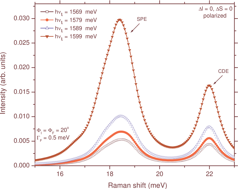
Figure 2: (Color online) Polarized monopolar Raman spectrum below band gap ($\Gamma_{f}=0.5$ meV).

We show in Fig. 2 the polarized Raman spectrum for monopole final state excitations, computed with $\Gamma_{f}=0.5$ meV. $E^{\prime}_{gap}$ in this situation is 1599.2 meV. The incident (and backscattered) angle is equal to $20^{\circ}$. $h\nu_{i}$ is swept in a 30 meV interval below $E^{\prime}_{gap}$. Notice the monotonic increase of intensities as $h\nu_{i}$ rises. One peak corresponding to the CDE, and a second one related to the SPEs are observed. In the latter case, there is a group of energy levels contributing to the peak in the figure. We may think of this set of levels as a Coulomb-renormalized oscillator shell. As we are dealing with monopole excitations, the average position of the group should correspond to $2\hbar\omega^{\prime}_{0}$, i.e., the renormalized oscillator energy is $\hbar\omega^{\prime}_{0}\approx 9$ meV.

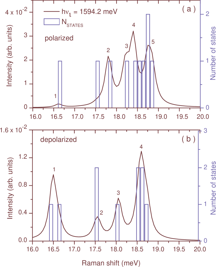
Figure 3: (Color online) Polarized and depolarized monopolar Raman spectra ($\Gamma_{f}=0.1$ meV) and comparison with the density of energy levels.

The fine structure of the SPE peak is shown in Fig. 3a along with the density of final-state energy levels. In this case, the monopolar polarized Raman spectrum was calculated with $\Gamma_{f}=0.1$ meV. The depolarized spectrum is shown in Fig. 3b (In fact, only the energy interval corresponding to the SPE peak is shown. The SDE peak is outside this interval). Histograms with a step of 0.1 meV are used to represent the level density. Although Eq. (4) refers to collective excitations, we have used its implications to correlate the polarized Raman spectrum with the level density of charge monopolar SPEs, and the depolarized spectrum with the density of monopolar spin excitations. The Raman spectra reproduce quite accurately the details of the level density in both cases. A general remark concerning Fig. 3 is that the intensity of the depolarized peaks is about three times lower than the intensity of the polarized ones.

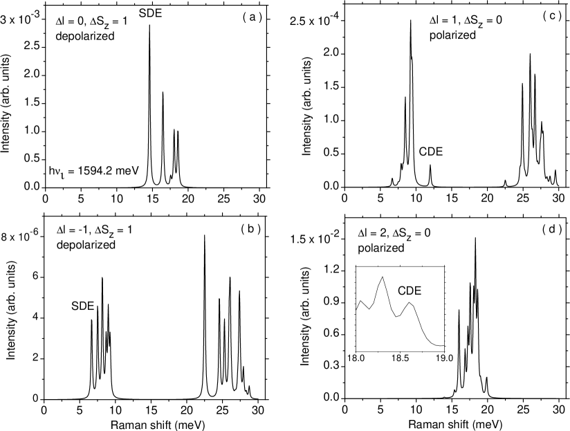
Figure 4: Raman spectra in different channels ($\Gamma_{f}=0.1$ meV). The incident laser energy is $1594.2$ meV.

Depolarized spectra for spin-flipped monopolar and dipolar final states are shown in Figs. 4a and b. Polarized spectra for dipolar and quadrupolar states are shown in Figs. 4c and d. The shell structure Lockwood2 ; Heitmann is clearly seen in these figures. Dipolar and spin-flipped final states are strongly depressed in the Raman spectra. Quadrupole final states, on the contrary, show magnitudes comparable to monopolar peaks.

The fact that even multipoles are favored in the Raman spectra is understood in terms of the even parity of final states in a two-photon process. On the other hand, spin-flipped final states are reached only as a consequence of valence-band mixing. We (virtually) create an electron and a hole, whose dominant component is $m_{j}$, and annihilate the same hole and an electron with opposite spin. The amplitude of the latter process is proportional to the minority component of the hole wave function, $\chi_{m^{\prime}_{j}}$. It means that the amplitude squared $|A_{fi}|^{2}$ will be proportional to $|\chi_{m^{\prime}_{j}}|^{2}$.

These calculations show that experimental measurements of the electronic Raman spectra with below band gap excitation can provide valuable information on the collective states and SPEs of qdots. Furthermore, below band gap excitation can overcome the problem of overlap with the intense photoluminescence observed under resonant excitation. The peak maxima exhibit a continuous but not very marked increase in intensity with excitation approaching the band gap (see Fig. 2), indicating that excitation around 30 meV below the gap is sufficient. The other notable feature of these calculations, apart from the marked differences predicted in Raman intensities of the polarized and depolarized multipolar components, is the fine structure of the SPE Raman peak (see Fig. 3). It would be interesting to probe all these aspects experimentally.

III.2 The extreme resonance region

In the present section, we consider Raman scattering when $h\nu_{i}$ moves in a 30 meV window above $E^{\prime}_{gap}$. We will call this interval the “extreme resonance” window.

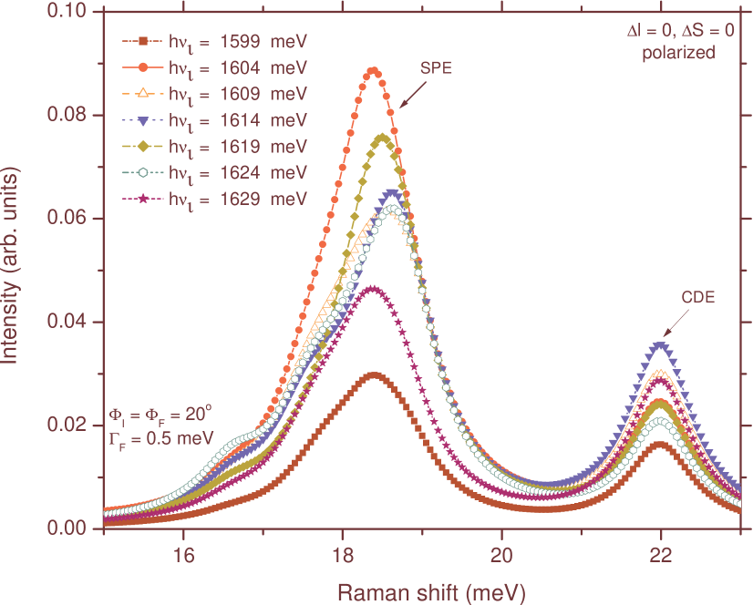
Figure 5: (Color online) Monopolar polarized Raman spectra ($\Gamma_{f}=0.5$ meV) in the extreme resonance region: $E^{\prime}_{gap}<h\nu_{i}<E^{\prime}_{gap}+30$ meV.

Fig. 5 shows a polarized Raman spectrum corresponding to charge monopolar final states. As in Fig. 2, we used $\Gamma_{f}=0.5$ meV. Two characteristics of Fig. 5 make it very different from Fig. 2: (i) Peak intensities are not monotonous with respect to variations of $h\nu_{i}$, and (ii) The position of the maximum in the SPE peak moves slightly with $h\nu_{i}$. Both properties are related to resonances in the intermediate states.

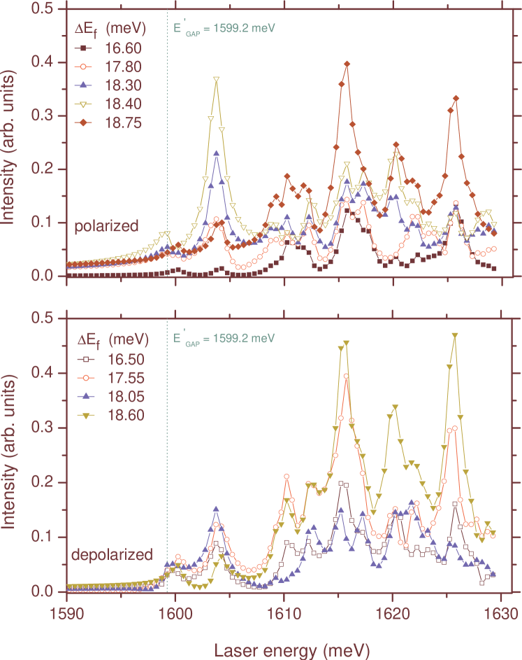
Figure 6: (Color online) The dependence on $h\nu_{i}$ of the intensity of SPE peaks identified in Fig. 3.

Resonances in the intermediate states can be better visualized if we follow the Raman intensities of the peaks shown in Fig. 3. For this purpose, we computed monopolar Raman spectra with $\Gamma_{f}=0.1$ meV and varying $h\nu_{i}$ with a 0.5 meV step. The results are drawn in Fig. 6. The monotonous increase of peaks in the $h\nu_{i}<E^{\prime}_{gap}$ region is apparent in the figure. On the other hand, for $h\nu_{i}>E^{\prime}_{gap}$ the intensity variation with laser excitation energy is much more complicated. The intensities of the individual SPE components rise and fall markedly with laser energy, as has been observed experimentally. This variation is attributed to individual resonances occurring within intermediate states lying close to the band gap as the incident light energy sweeps through them. The effect is particularly noticeable for $h\nu_{i}\approx 1616$ and 1626 meV. In the associated intermediate states, the added e-h pair has zero total angular momentum projection, and the hole is basically a heavy hole. Notice that the same intermediate states are responsible for the strong enhancement of Raman intensities in both the polarized and depolarized geometries.

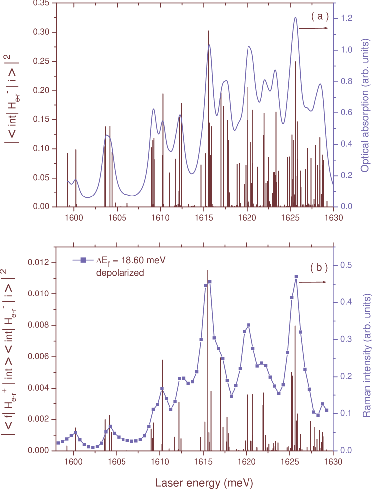
Figure 7: (Color online) (a) Absorption in the model qdot. (b) Intensity of the spin monopolar Raman peak with $\Delta E_{f}=18.6$ meV as a function of $h\nu_{i}$.

A spin monopolar SPE Raman peak is followed as a function of $h\nu_{i}$ in Fig. 7b. For comparison, we have also given the products $|\langle f|\hat{H}^{+}_{e-r}|int\rangle\langle int|\hat{H}^{-}_{e-r}|i\rangle|^{2}$ for each intermediate state, and the absorption strengths $|\langle int|\hat{H}^{-}_{e-r}|i\rangle|^{2}$ (the upper panel). The optical absorption coefficient is defined according to

$$\alpha(E)=\sum_{int}|\langle int|\hat{H}^{-}_{e-r}|i\rangle|^{2}\frac{\Gamma_{int}/\pi}{(E-E_{int})^{2}+\Gamma_{int}^{2}}.$$ (32)

Fig. 7 shows that, in the present situation, peaks in the optical absorption coincide with peaks in the Raman intensities, which leads to the conclusion that the latter are related to incoming (absorption) resonances. Note that from Fig. 7b it follows that interference effects among intermediate states are weak in the Raman scattering under extreme resonanceJPCM . Raman spectra in the extreme resonance region look similar to the spectra shown in Fig. 4, but with SPE peaks much higher than collective ones and selectively enhanced for particular values of $h\nu_{i}$. A comparison with the density of energy levels would lead to results very similar to those of Fig. 3.

III.3 Raman spectra 40 meV above band gap

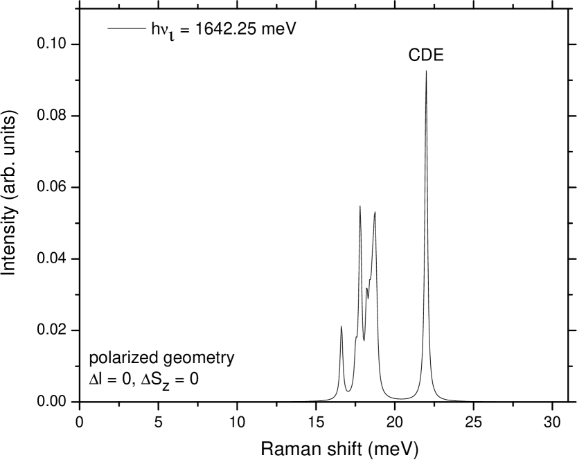
Figure 8: Raman spectrum in the polarized geometry ($\Gamma_{f}=0.1$ meV) for well above band gap excitation.

As mentioned in Section IIG, we assume that $\Gamma_{int}$ experiences a sudden increase when $E_{int}>E^{\prime}_{gap}+\hbar\omega_{LO}$. As a result, the contribution of these states to $A_{fi}$, Eq. (1), loses its resonant character even when $h\nu_{i}$ sweeps this energy range. It means that peak intensities become smooth functions of $h\nu_{i}$, as for below band gap excitation. Both collective and SPE Raman peaks decrease in intensity for $h\nu_{i}>E^{\prime}_{gap}+\hbar\omega_{LO}$ (as compared with values at extreme resonance), but the SPE peaks are more strongly depressed JPCM . Fig. 8 shows a typical spectrum at $h\nu_{i}=1642$ meV.

Nevertheless, a modest increase of the peak intensity for $h\nu_{i}$ well above the band gap may result not only from large values of $|\langle f|\hat{H}^{+}_{e-r}|int\rangle\langle int|\hat{H}^{-}_{e-r}|i\rangle|^{2}$ but also from relatively small level broadening (as compared with the neighboring levels). There could be a set of intermediate states in which $\Gamma_{int}$ takes relatively small values. One can think, for example, of the lowest state in a sub-band, let us say the $k_{z}=2$ electron sub-band. Inter sub-band transitions due to phonon emission are not as fast as intra sub-band transitions Shah . Consequently, the $\Gamma_{int}$ of the lowest state in the sub-band is relatively small. We will call these states “excitonic” states, X. If the product $\langle f|\hat{H}^{+}_{e-r}|X\rangle\langle X|\hat{H}^{-}_{e-r}|i\rangle$ is not small, a peak in the Raman intensity will appear. In the interpretation of Ref. Danan, , this is an “incoming” resonance.

On the other hand, “outgoing” resonances correspond to emitted photons with energy $E_{X}$, as shown in Fig. 9. The intermediate states are located at excitation energies $E_{X}+E_{f}$. One can think of these states as an exciton on top of a collective excitation or, conversely, a collective electronic excitation on top of an exciton Lozovik . The $X$ in this case may correspond to an absorption peak in the extreme resonance region or well above band gap.

The resonant enhancement of these “exciton plus plasmon” states can be due, again, to big numerators or small denominators in Eq. (1). Relatively small $\Gamma_{int}$ could be related to the collective nature of these states or to the relative isolation from neighboring levels.

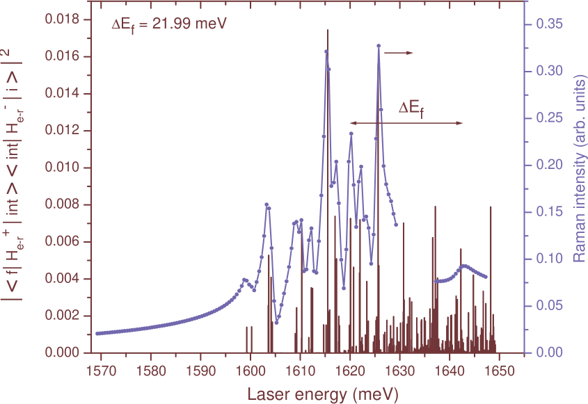
Figure 10: (Color online) Intensity of the CDE monopolar Raman peak as a function of $h\nu_{i}$. An outgoing resonance at 1642 meV is modelled.

To illustrate the effect of resonant enhancement of Raman peaks, we show in Fig. 10 the intensity of the CDE peak as a function of $h\nu_{i}$. The entire range of variation is shown for completeness, i.e., below band gap excitation, extreme resonance, and well above band gap excitation. In the extreme resonance case, the enhancement is related to absorption maxima as mentioned above. On the other hand, for $h\nu_{i}$ well above band gap, we pick up an intermediate state with energy $E_{X}+E_{CDE}$, where the exciton level $X$ corresponds to the absorption maximum at 1620 meV (see Fig. 7a), and $E_{CDE}\approx 22$ meV is the energy of the charge monopolar collective state. For this state, we chose $\Gamma_{int}=2$ meV. The effect is an enhancement of the intensity around 1642 meV, as shown in the figure, that according to Ref. Danan, is an outgoing resonance.

This calculation reveals that the dependence of $\Gamma_{int}$ on $E_{int}$ may dictate the qualitative features of Raman scattering with well above band gap excitation. A consistent treatment in which the $\Gamma_{int}$ are computed for each $|int\rangle$ is left for future study.

IV Conclusions

This theoretical investigation of the role of resonance excitation in electronic Raman scattering from qdots has revealed many hitherto unsuspected features and details. In general terms, the Raman intensities of the SPEs, CDEs, and SDEs are strongly affected when the incident light energy is swept from below, through, and above the quantum dot band gap. Incoming resonances produce a rapid variation in intensity for excitation energies just above the band gap, and outgoing resonances are predicted for higher excitation energies, as observed experimentally. In fact, observation of the Raman intensity of just one SPE, for example, as a function of the incident light energy can provide precise details of the optical absorption spectrum and density of states. The role of damping in the intermediate states has been shown to be a significant factor in determining these resonances and deserves further theoretical analysis.

Another aspect of this work is the unravelling of the complexity of features in polarized Raman spectroscopy of qdots. This spectral complexity in dots with large numbers of electrons has been evident from the first experiments. These calculations have shown what excitations dominate in which polarizations and point the way to a better control of what is measured in future experiments.

Experimentally, the predicted selective resonances have advantages and disadvantages. By employing resonance excitation, a particular final state can be enhanced over its companions and thus make it easier to identify. On the other hand, the rapid variation in intensity of the individual and numerous SPEs makes it difficult to uniquely identify them. In this regard, the fine structure evident for SPEs from these calculations should be explored by performing high resolution Raman spectroscopy in future. The best situation for evaluating the SPEs would be for an excitation energy about 30 meV below the band gap, where some overall resonance enhancement occurs but the contribution from band gap photoluminescence would be weak. No such experiments have been performed to date.

Appendix A Matrix elements of the Kohn-Luttinger Hamiltonian

In the present appendix, we give the matrix elements of the Kohn-Luttinger Hamiltonian entering Eq. (10). Results are presented for the more general case when a magnetic field, $B$, is applied in the $z$ direction. We use the following set of parameters parameters :

$$\gamma_{1}=6.790,\quad\gamma_{2}=1.924,\quad\gamma_{3}=2.681,$$

$$\bar{\gamma}=(\gamma_{2}+\gamma_{3})/2,\quad\kappa=1.2,\quad q=0.04$$

The Kohn-Luttinger Hamiltonian has the following structure in the $m_{j}$ variable:

$$\cal{H}_{KL}=\left(\begin{array}[]{cccc}H_{3/2}&S&R&0\\ S^{\dagger}&H_{1/2}&0&R\\ R^{\dagger}&0&H_{-1/2}&-S\\ 0&R^{\dagger}&-S^{\dagger}&H_{-3/2}\end{array}\right)$$ (37)

The $H$ terms are diagonal in oscillator and $k_{z}$ indexes. They are given by:

$$H_{\pm 3/2}=\hbar\Omega_{e}\frac{m_{e}(\gamma_{1}+\gamma_{2})}{m_{0}}(2k+|l_{h}|+1)+\frac{\hbar^{2}}{2m_{0}}(\gamma_{1}-2\gamma_{2})\frac{k_{z}^{2}\pi^{2}}{L^{2}}-\frac{\hbar\omega_{ce}}{2}\frac{m_{e}(\gamma_{1}+\gamma_{2})}{m_{0}}l_{h}\pm\mu_{B}\left(3\kappa+\frac{27q}{4}\right)B,$$ (38)

$$H_{\pm 1/2}=\hbar\Omega_{e}\frac{m_{e}(\gamma_{1}-\gamma_{2})}{m_{0}}(2k+|l_{h}|+1)+\frac{\hbar^{2}}{2m_{0}}(\gamma_{1}+2\gamma_{2})\frac{k_{z}^{2}\pi^{2}}{L^{2}}-\frac{\hbar\omega_{ce}}{2}\frac{m_{e}(\gamma_{1}-\gamma_{2})}{m_{0}}l_{h}\pm\mu_{B}\left(\kappa+\frac{q}{4}\right)B,$$ (39)

where $m_{0}$ is the electron mass in vacuum, $\mu_{B}$ is the atomic Bohr magneton, $\omega_{ce}$ is the electron cyclotron frequency, $\Omega_{e}=\sqrt{\omega_{0}^{2}+\omega_{ce}^{2}/4}$, and $k$, $l_{h}$ are the radial and angular momentum quantum numbers corresponding to the 2D oscillator state.

The matrix elements of the $S$ and $R$ operators are written in the following form:

$$\langle k,l_{h},k_{z}|S|k^{\prime},l^{\prime}_{h},k^{\prime}_{z}\rangle = \frac{\sqrt{3}\hbar^{2}\gamma_{3}}{m_{0}}\sqrt{\frac{m_{e}\Omega_{e}}{\hbar}}\frac{4k_{z}k^{\prime}_{z}}{L(k_{z}^{2}-k_{z}^{{}^{\prime}2})}\delta_{l_{h},l^{\prime}_{h}+1}\delta_{k_{z}+k^{\prime}_{z},odd}$$ (43)

$$\times \left\{\begin{array}[]{ll}\sqrt{k^{\prime}+1}\left(1-\omega_{ce}(2\Omega_{e})\right)\delta_{k,k^{\prime}+1}+\sqrt{k^{\prime}+|l^{\prime}_{h}|}\left(1+\omega_{ce}/(2\Omega_{e})\right)\delta_{k,k^{\prime}};&l^{\prime}_{h}\leq-1\\ &\\ \sqrt{k^{\prime}}\left(1+\omega_{ce}/(2\Omega_{e})\right)\delta_{k,k^{\prime}-1}+\sqrt{k^{\prime}+l^{\prime}_{h}+1}\left(1-\omega_{ce}/(2\Omega_{e})\right)\delta_{k,k^{\prime}};&l^{\prime}_{h}\geq 0,\end{array}\right.$$

$$\langle k,l_{h},k_{z}|R|k^{\prime},l^{\prime}_{h},k^{\prime}_{z}\rangle = \frac{\sqrt{3}\bar{\gamma}m_{e}}{2m_{0}}\hbar\Omega_{e}\delta_{l_{h},l^{\prime}_{h}+2}\delta_{k_{z},k^{\prime}_{z}}$$ (49)

$$\times \left\{\begin{array}[]{ll}\sqrt{(k^{\prime}+|l^{\prime}_{h}|-1)(k^{\prime}+|l^{\prime}_{h}|)}\left(1+\omega_{ce}/(2\Omega_{e})\right)^{2}\delta_{k,k^{\prime}}&\\ &\\ 2\sqrt{(k^{\prime}+1)(k^{\prime}+|l^{\prime}_{h}|)}\left(1-\left(\omega_{ce}/(2\Omega_{e})\right)^{2}\right)\delta_{k,k^{\prime}+1};&l^{\prime}_{h}\leq-2\\ &\\ \sqrt{(k^{\prime}+2)(k^{\prime}+1)}\left(1-\omega_{ce}/(2\Omega_{e})\right)^{2}\delta_{k,k^{\prime}+2}&\end{array}\right.$$

$$\times \left\{\begin{array}[]{ll}-\sqrt{k^{\prime}(k^{\prime}+1)}\left(1+\omega_{ce}/(2\Omega_{e})\right)^{2}\delta_{k,k^{\prime}-1}&\\ &\\ -2k^{\prime}\left(1-\left(\omega_{ce}/(2\Omega_{e})\right)^{2}\right)\delta_{k,k^{\prime}};&l^{\prime}_{h}=-1\\ &\\ -\sqrt{(k^{\prime}+2)(k^{\prime}+1)}\left(1-\omega_{ce}/(2\Omega_{e})\right)^{2}\delta_{k,k^{\prime}+1}&\end{array}\right.$$ (55)

$$\times \left\{\begin{array}[]{ll}\sqrt{(k^{\prime}-1)k^{\prime}}\left(1+\omega_{ce}/(2\Omega_{e})\right)^{2}\delta_{k,k^{\prime}-2}&\\ &\\ 2\sqrt{k^{\prime}(k^{\prime}+|l^{\prime}_{h}|+1)}\left(1-\left(\omega_{ce}/(2\Omega_{e})\right)^{2}\right)\delta_{k,k^{\prime}-1};&l^{\prime}_{h}\geq 0\\ &\\ \sqrt{(k^{\prime}+l^{\prime}_{h}+2)(k^{\prime}+l^{\prime}_{h}+1)}\left(1-\omega_{ce}/(2\Omega_{e})\right)^{2}\delta_{k,k^{\prime}}.&\end{array}\right.$$ (61)

$\sigma\backslash~{}m_{j}$	3/2	1/2	-1/2	-3/2
1/2	$\varepsilon_{+i}$	$\sqrt{2/3}\;\varepsilon_{zi}$	$\sqrt{1/3}\;\varepsilon_{-i}$	0
-1/2	0	$\sqrt{1/3}\;\varepsilon_{+i}$	$\sqrt{2/3}\;\varepsilon_{zi}$	$\varepsilon_{-i}$

Table 1: The quotient $\vec{\varepsilon}_{i}\cdot\vec{p}_{\sigma,m_{j}}/(iP)$, where $P$ is the GaAs band constant.

Figure 1: Spectrum of final states in the model qdot.

Figure 9: Schematic representation of incoming and outgoing Raman resonances.

References

- (1) M. Cardona (ed.), Light scattering in solids, 2nd edition, (Springer-Verlag, New-York, 1982).
- (2) M. Cardona and G. Guntherodt (eds.), Light scattering in solids IV (Springer-Verlag, New-York, 1984).
- (3) D.J. Lockwood and J.F. Young (eds.), Light scattering in semiconductor structures and superlattices (Plenum, New-York, 1991).
- (4) R. Loudon, Adv. Phys. 13, 423 (1964).
- (5) Strictly speaking, there are two second-order terms contributing to the Raman scattering, one like in Eq. (1), and a second term, which has a similar structure but with a different energy denominator: meV. text Our calculations including both terms have shown that the contribution from the second one is insignificant in the present case.
- (6) A.R. Goni, A. Pinczuk, J.S. Weiner, J.M. Calleja, B.S. Dennis, L.N. Pfeiffer, and K.W. West, Phys. Rev. Lett. 67, 3298, (1991); C. Schuller, G. Biese, K. Keller, C. Steinebach, and D. Heitmann,P. Grambow, K. Eberl Phys. Rev. B 54, 17304 (1996); A. Pinczuk, B.S. Dennis, L.N. Pfeiffer, and K.W. West, Philos. Mag. B 70, 429 (1994).
- (7) Daw-Wei Wang and S. D. Sarma, Phys. Rev. B 65, 125322 (2002).
- (8) G. Danan, A. Pinczuk, J.P. Valladares, L.N. Pfeiffer, K.W. West, and C.W. Tu, Phys. Rev. B 39, 5512 (1989).
- (9) C.M. Sotomayor-Torres, D.J. Lockwood, and P.D. Wang, J. Electr. Materials 29, 576 (2000).
- (10) C. Schuller, K. Keller, G. Biese, E. Ulrichs, L. Rolf, C. Steinebach, D. Heitmann, and K. Eberl, Phys. Rev. Lett. 80, 2673 (1998).
- (11) M. Barranco, L. Colletti, A. Emperador,E. Lipparini, M. Pi, and L. Serra, Phys. Rev. B 61, 8289 (2000).
- (12) L. Wendler, V.M. Fomin, A.V. Chaplik, and A.O. Govorov, Phys. Rev. B 54, 4794 (1996).
- (13) C. Steinebach, C. Schuller, and D. Heitmann, Phys. Rev. B 59, 10240 (1999).
- (14) A. Delgado, A. Gonzalez and E. Menendez-Proupin, Phys. Rev. B 65, 155306 (2002).
- (15) L. Jacak, P. Hawrylak, and A. Wojs, Quantum dots, (Springer-Verlag, Berlin, 1998).
- (16) A. Delgado, L. Lavin, R. Capote, and A. Gonzalez, Physica E (Amsterdam) 8, 342 (2000).
- (17) A.H. MacDonald, G.C. Aers, Phys. Rev. B 29, 5976 (1984).
- (18) P. Ring and P. Schuck, The Nuclear Many-Body Problem (Springer-Verlag, New-York, 1980).
- (19) J. Shah, Ultrafast spectroscopy of semiconductors and semiconductor nanostructures (Springer-Verlag, New-York, 1999).
- (20) To reproduce the experimental conditions of paper [Heitmann, ], a harmonic confinement, of around 6 meV should be taken. However, we choose a higher value, 12 meV, in order to be closer to the strong confinement situation holding for self-assembled qdotsHawrylak , which is the immediate interest of planned experiments.
- (21) D.J. Lockwood, P. Hawrylak, P.D. Wang, C.M. Sotomayor Torres, A. Pinczuk, and B.S. Dennis, Phys. Rev. Lett. 77, 354 (1996).
- (22) A. Delgado, A. Gonzalez, J. Phys.: Condens. Matter 15, 4259 (2003).
- (23) The experimental observation of outgoing resonances in Ref. Danan, raises the question about the existence of special intermediate states with energy (see Fig. 9), where both (an exciton state), and (a final collective state) are exact eigenstates of the Hamiltonian. This fact suggests the existence of a hidden or approximate symmetry as in the case of electron-hole systems in a strong magnetic field. See, for example, I.V. Lerner and Yu.E. Lozovik, Sov. Phys.: Solid State 25, 874 (1983).
- (24) L.W. Molenkamp, R. Eppenga, G.W. t’Hooft, P. Dawson, C.T. Foxon, and K.J. Moore, Phys. Rev. B 38, 4314 (1988).