Also at ]Dept. of Chemistry, University of Fribourg, 1700 Fribourg, Switzerland

Ab-inito Linear Scaling Response Theory:
Electric Polarizability by Perturbed Projection

Abstract

A linear scaling method for calculation of the static ab inito response within self-consistent field theory is developed and applied to calculation of the static electric polarizability. The method is based on density matrix perturbation theory [Niklasson and Challacombe, PRL (LJ9425)], obtaining response functions directly via a perturbative approach to spectral projection. The accuracy and efficiency of the linear scaling method is demonstrated for a series of three-dimensional water clusters at the RHF/6-31G** level of theory. Locality of the response under a global electric field perturbation is numerically demonstrated by approximate exponential decay of derivative density matrix elements.

Linear scaling methods that reduce the computational complexity of electronic structure calculations to ${\cal O}(N)$, where $N$ is system size, impact disciplines that demand quantum simulation of increasingly large and complex systems Galli (1996); Bowler et al. (1997); Goedecker (1999); Ordejon (2000); Gogonea et al. (2001); Wu and Jayanthi (2002). To date, the most successful and prolific applications of linear scaling technologies are ground state studies involving empirical model Hamiltonians. To a lesser degree, ground state applications using ab initio models with $N$-scaling contribute to a variety of fields, typically at the Self-Consistent-Field (SCF) level of theory and requiring in some cases parallel implementations to reach levels of applicability comparable with empirical models. These SCF theories include the Hartree-Fock (HF), Kohn-Sham Density Functional (DF) and hybrid HF/DF models.

Beyond ground state methods, little attention has been given to linear scaling algorithms for the computation of dynamic and static response properties; the latter including the nuclear magnetic shielding tensor Wolinski et al. (1990), the rotational g-tensor Gauss et al. (1996), indirect spin-spin coupling constant Pennington and Slichter (1991); Malkina et al. (1996), third order properties such as the first hyperpolarizability van Gisbergen et al. (1997) and polarizability derivatives such as the Raman intensity Lazzeri and Mauri (2003); Quinet and Champagne (2001). Dynamic properties may be computed using linear scaling algorithms to propagate the density matrix Nomura et al. (1997); Yam et al. (2003) in the time domain, followed by convolution to obtain the spectral response. In this way, Yam, Yokojima and Chen Yam et al. (2003) have recently demonstrated linear scaling computation of the absorption spectra for one-dimensional polymers at the local density level of theory, but requiring $\sim 14,000$ time steps. In the static zero frequency limit, solving the coupled-perturbed self-consistent-field (CPSCF) equations using standard algorithms is likewise difficult for large systems. Several algorithms have therefore been proposed for solving the CPSCF equations that may be capable of achieving a reduced scaling better than ${\cal O}(N^{3})$ Ochsenfeld and Head-Gordon (1997a); Larsen et al. (2001a).

In this letter, we develop the density matrix perturbation theory of Niklasson and Challacombe Niklasson and Challacombe (2004) for $N$-scaling solution of the ab initio CPSCF equations, and demonstrate the early onset of linear scaling for the accurate calculation of the first electric polarizability of three-dimensional systems using large basis sets. This perturbed projection method is general and can be extended to a variety of static properties.

Algorithms for linear scaling self-consistent-field (SCF) theory exploit the quantum locality of non-metallic systems, manifested in the approximate exponential decay of the density matrix with atom-atom separation, through the effective use of sparse matrix methods and iterative approaches to spectral projection Niklasson (2002); Niklasson et al. (2003). This quantum locality should, in principle, extend also to the derivative density matrices central to the CPSCF equations. Indeed, exponential decay of the derivative density matrix within ab initio SCF theory has been demonstrated numerically for local nuclear displacement Ochsenfeld and Head-Gordon (1997b). However, standard approaches to the CPSCF equations Pople et al. (1979); Sekino and Bartlett (1986); Karna and Dupuis (1991) do not admit exploitation of this locality, as they are based on perturbation of the wave function, requiring ${\cal O}(N^{3})$ eigensolution and typically ${\cal O}(N^{5})$ transformation of two-electron integrals into the eigenbasis. Avoiding both eigensolution and integral transformation, Ochsenfeld and Head-Gordon Ochsenfeld and Head-Gordon (1997b) and later Larsen et al. Larsen et al. (2001b) proposed iterative solutions to the CPSCF equations involving purely non-orthogonal representations. In both of these approaches, a linear system of equations containing commutation relations must be solved.

Recently, a formulation of density matrix perturbation theory has been proposed by Niklasson and Challacombe (NC) Niklasson and Challacombe (2004) that presents a new opportunity for solving the CPSCF equations within the context of linear scaling spectral projection Niklasson (2002); Niklasson et al. (2003). The new approach is based on the relationship between the density matrix $\mathcal{D}$ and the effective Hamiltonian or Fockian $\mathcal{F}$ through the spectral projector (Heaviside step function) $\mathcal{D}=\theta(\tilde{\mu}I-\mathcal{F})$, where the chemical potential $\tilde{\mu}$ determines the occupied states via Aufbau filling. Spectral projection can be carried out in a number of ways Niklasson (2002); Niklasson et al. (2003); McWeeny (1960); Clinton et al. (1969); Palser and Manolopoulos (1998); Beylkin et al. (1999); Nemeth and Scuseria (2000); Holas (2001), with perhaps the best know algorithm being McWeeny’s cubic purification scheme McWeeny (1960). More recently new recursive polynomial expansions of the projector have emerged, such as the second order trace correcting (TC2) Niklasson (2002) and fourth order trace resetting (TRS4) Niklasson et al. (2003) purification. These new methods (TC2 and TRS4) have convergence properties that depend only weakly on the band gap, do not require knowledge of the chemical potential and perform well for all occupation to state ratios. In the NC approach, the perturbation expansion is developed within the reference groundstate projector allowing order by order collection of terms at each iteration, establishing a quadratically convergent sequence for the response functions.

We now proceed with development of the perturbed projection approach, which will be outlined for the concrete case of perturbation by an electric field within the Hartree-Fock (HF) theory. However, the perturbed projection method is general and extensible to DF and hybrid HF/DF models, and to other static perturbations through high order.

In the following, the indexes $a,b,\dots$ refer to perturbation order, while $i,j,\dots$ mark the iteration count. The symbols $\mathcal{D},\mathcal{F},\dots$ are matrices in an orthogonal representation, while $D,F,\dots$ are the corresponding matrices in a non-orthogonal basis. The transformation between orthogonal and non-orthogonal representations is carried out in ${\cal O}(N)$ using congruence transformations Wilkinson (1965); Stewart (1973) provided by the AINV algorithm for computing sparse approximate inverse Cholesky factors Benzi and Meyer (1995); Benzi et al. (1996, 2001).

Within HF theory, the total electronic energy $E_{\rm tot}$ of a molecule in a static electric field $\mathcal{E}$ is

$$E_{\rm tot}(\mathcal{E})=Tr[D(h^{0}+\mu\mathcal{E})]+\frac{1}{2}Tr[D(J(D)+K(D))],$$ (1)

where $D$ is the density matrix in the electric field, $h^{0}$ is the core Hamiltonian, $\mu$ is the dipole moment matrix, $J(D)$ is the Coulomb matrix and $K(D)$ the exact HF exchange matrix. The total energy may be developed in the perturbation expansion

$$E_{\rm tot}(\mathcal{E})=E_{\rm tot}(0)+\sum_{a}\mu_{a}\mathcal{E}^{a}+\frac{1}{2}\sum_{ab}\alpha_{ab}\mathcal{E}^{a}\mathcal{E}^{b}+\dots,$$ (2)

where $\alpha_{ab}$ is the first order polarizability, $\mu_{a}$ is the dipole moment and $\mathcal{E}^{a}$ is the electric field in direction $a$. The polarizability is the second order response of the total energy with respect to variation in the electric field Sekino and Bartlett (1986)

$$\alpha_{ab}=-\frac{\partial^{2}E_{\rm tot}}{\partial\mathcal{E}^{a}\partial\mathcal{E}^{b}}\bigg{|}_{\mathcal{E}=0}=-2Tr[D^{a}\mu_{b}].$$ (3)

The first order density matrix derivative $\mathcal{D}^{a}$ in the $a$ direction is obtained by variation of both the spectral projector $\theta$ and the Fockian $\mathcal{F}=\mathcal{F}^{0}+\sum_{a}\mathcal{E}^{a}\mathcal{F}^{a}+\dots$ as

$$\mathcal{D}^{a}=\frac{\partial}{\partial\mathcal{E}^{a}}\theta(\tilde{\mu}I-(\mathcal{F}^{0}+\mathcal{E}^{a}\mathcal{F}^{a}))\bigg{|}_{\mathcal{E}=0}.$$ (4)

The HF Fockian $F^{0}$ in the non-orthogonal basis is $F^{0}=h^{0}+J(D^{0})+K(D^{0})$, where the Coulomb matrix $J$ may be computed in ${\cal O}(N{\rm lg}N)$ with a quantum chemical tree code (QCTC) Challacombe and Schwegler (1997) and the exchange matrix $K$ computed in ${\cal O}(N)$ with the ONX algorithm that exploits quantum locality of $D^{0}$ Schwegler et al. (1997). Likewise the derivative Fockian, $F^{a}=\mu_{a}+J(D^{a})+K(D^{a})$, may be computed with the same algorithms in linear scaling time if $D^{a}$ manifests decay properties similar to $D^{0}$. A similar equation holds for the derivative Fockian within DF and hybrid HF/DF theories with addition of the exchange-correlation matrix $V_{xc}^{a}(D^{0},D^{a})$ Lee and Colwell (1994).

In our approach to linear scaling computation of the polarizability $\alpha_{ab}$, the ground state density matrix $\mathcal{D}^{0}$ is computed using a spectral projection algorithm such as TC2 Niklasson (2002) in conjunction with sparse atom-blocked linear algebra Niklasson et al. (2003); Challacombe (2000). Linear scaling is achieved for insulating systems through the dropping (filtering) of atom-atom blocks with Frobenious norm below a numerical threshold ($\sim 10^{-4}-10^{-6}$). At SCF convergence the TC2 algorithm generates a polynomial sequence defining the groundstate projector, from which expansion of the derivative density matrix can be obtained term by term.

The derivative density matrix and derivative Fockian depend on each other implicitly and must be solved for self-consistently via the coupled-perturbed self-consistent-field (CPSCF) equations. The necessary and sufficient criteria for convergence of the CPSCF equations are $[\mathcal{F}^{a},\mathcal{D}^{0}]+[\mathcal{F}^{0},\mathcal{D}^{a}]=0$ and $\mathcal{D}^{a}=\mathcal{D}^{a}\mathcal{D}^{0}+\mathcal{D}^{0}\mathcal{D}^{a}$ Furche (2001). Solution of the CPSCF equations with perturbed projection involves the steps

$$F^{a}_{n}=\mu_{a}+J(D^{a}_{n})+K(D^{a}_{n})$$ (5a)

$$\displaystyle\widetilde{F}^{a}_{n}=\sum_{k=n-m}^{n}c_{k}F^{a}_{k}$$ (5b)

$$\displaystyle\mathcal{D}^{a}_{n+1}=\frac{\partial}{\partial\mathcal{E}^{a}}\theta(\tilde{\mu}I-(\mathcal{F}^{0}+\mathcal{E}^{a}\widetilde{\mathcal{F}}^{a}_{n}))\bigg{|}_{\mathcal{E}=0}$$ (5c)

with starting point $D^{a}_{0}=0$. In step (5a), $F^{a}_{n}$ is constructed in ${\cal O}(N)$ using the QCTC Challacombe and Schwegler (1997) and ONX Schwegler et al. (1997) algorithms in MondoSCF Challacombe et al. (2001). Next, Weber and Daul’s DDIIS algorithm for convergence acceleration of the CPSCF equation Weber and Daul (2003) is used to optimize the $c_{k}$ coefficients in step (5b), keeping the last $m$ steps in the extrapolation. Then, the density matrix derivative $\mathcal{D}^{a}_{n+1}$ is obtained in step (5c) as $\mathcal{D}^{a}_{n+1}=\lim_{i\to\infty}\mathcal{X}^{a}_{i}$ via the NC density matrix perturbation theory, based on the TC2 projector:

$$\left.\begin{array}[]{ll}\mathcal{X}^{a}_{i+1}&=\mathcal{X}^{a}_{i}\mathcal{X}^{0}_{i}+\mathcal{X}^{0}_{i}\mathcal{X}^{a}_{i}\\ \mathcal{X}^{0}_{i+1}&=(\mathcal{X}^{0}_{i})^{2}\end{array}\right\}\quad{\rm Tr}[\mathcal{X}^{0}_{i}]\geq N_{e}$$ (6)

or

$$\left.\begin{array}[]{ll}\mathcal{X}^{a}_{i+1}&=2\mathcal{X}^{a}_{i}-\mathcal{X}^{a}_{i}\mathcal{X}^{0}_{i}-\mathcal{X}^{0}_{i}\mathcal{X}^{a}_{i}\\ \mathcal{X}^{0}_{i+1}&=2\mathcal{X}^{0}_{i}-(\mathcal{X}^{0}_{i})^{2}\end{array}\right\}\quad{\rm Tr}[\mathcal{X}^{0}_{i}]<N_{e}.$$ (7)

The matrices initiating the sequence are obtained from $\mathcal{F}^{0}$ and $\mathcal{F}^{a}$ by appropriately compressing their spectrum into the domain of convergence Niklasson (2002) using

$$\mathcal{X}^{0}_{0}=\frac{\mathcal{F}_{max}-\mathcal{F}^{0}}{\mathcal{F}_{max}-\mathcal{F}_{min}}~{}{\rm and}~{}\mathcal{X}^{a}_{0}=\frac{\mathcal{F}^{a}_{n}}{\mathcal{F}_{min}-\mathcal{F}_{max}},$$ (8)

where $\mathcal{F}_{min}$ and $\mathcal{F}_{max}$ are approximate upper and lower bounds to the eigenvalues of $\mathcal{F}^{0}$.

Recursion of the perturbed projection sequence is stopped when the change $\left|\mathcal{X}^{a}_{i+1}-\mathcal{X}^{a}_{i}\right|$ becomes small. Having solved for $D^{a}_{n}$, the next Fock matrix derivative $F^{a}_{n+1}$ is built, and the iteration continues until self-consistency, when the density matrix derivative $D^{a}_{n}$ and the desired property (e.g. the polarizability $\alpha_{ab}=-2Tr[D^{a}_{n}\mu_{b}]$) have reached a sufficient level of accuracy.

Figure 1: Total CPU time of the fifth CPSCF iteration for the water cluster sequence with the 6-31G and 6-31G** basis sets and the GOOD and TIGHT numerical thresholds (see text) controlling numerical precision of the result. The lines are fits to the last three and four points, respectively.

We have implemented these methods in the MondoSCF suite of linear scaling quantum chemistry programs Challacombe et al. (2001), and performed polarizability calculations on a series of water clusters up to (H₂O)₁₅₀. These clusters were obtained by carving a spherical region out of a snapshot from a periodic classical molecular dynamics simulation of water at standard liquid density, and have been used previously in a number of scaling tests Niklasson et al. (2003); Challacombe and Schwegler (1997); Schwegler et al. (1997).

Calculations have been carried out at both the RHF/6-31G and RHF/6-31G** levels of theory and with both the GOOD and TIGHT thresholding parameter sets that control precision of the linear scaling algorithms, corresponding to matrix thresholds of $10^{-5}$ and $10^{-6}$, respectively. These calculations were carried out on a single Intel Xeon 2.4GHz processor running RedHat Linux 8.0 and executables compiled with Portland Group Fortran Compiler pgf90 4.0-2 The Portland Group (2002). In Fig. 1, the total CPU time for the fifth CPSCF cycle (including build time for $\mathcal{F}^{a}$, iterative construction of $\mathcal{D}^{a}$ and all intermediate steps including congruence transformation) is shown for the RHF/6-31G and RHF/6-31G** series of water clusters. Convergence of the CPSCF equations for these systems are typically achieved in about 10 cycles, independent of cluster size, basis set or matrix threshold. In Table 1, the corresponding average water cluster polarizabilities computed with the MondoSCF algorithms are listed and compared to the those obtained with the GAMESS quantum chemistry package Schmidt et al. (1993) at the RHF/6-31G level of theory. Figure 2 shows the magnitude of density matrix derivative atom-atom blocks as a function of atom-atom distance under global perturbation by a static electric field.

Table 1: Average polarizabilities $\bar{\alpha}=(\alpha_{xx}+\alpha_{yy}+\alpha_{zz})/3N_{H_{2}0}$ in a.u. for a sequence of water clusters at the RHF/6-31G and RHF/6-31G** levels of theory. A comparison is made between results obtained with the GAMESS quantum chemistry program Schmidt et al. (1993) and those calculated with MondoSCF using different numerical approximations (see text) controlling precision of the linear scaling algorithms.

	6-31G	6-31G		6-31G**b
$N_{H_{2}0}$		GOOD	TIGHT	GOOD	TIGHT
10	4.569083	4.569918	4.569102	5.479161	5.479049
30	4.673213	4.673208	4.673227	5.585293	5.585280
50	4.703540	4.703512	4.703568	5.623057	5.622830
70	$-$	4.732207	4.732279	5.654646	5.654747
90	$-$	4.775002	4.775024	5.695435	5.695564
110	$-$	4.780718	4.780809	5.698338	5.698447
130	$-$	4.786383	4.786437	5.704859	5.704947
150	$-$	4.775124	4.775231	5.693268	5.693447

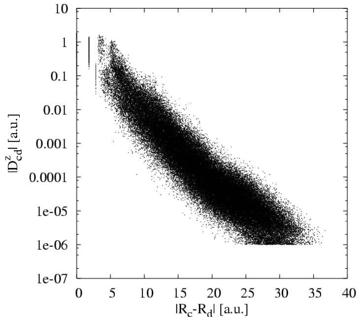
Figure 2: Magnitudes of atom-atom blocks of the RHF/6-31G density matrix derivative in the z direction with the separation of basis function centers for $(H_{2}O)_{150}$. The density matrix derivative has been converged using a TIGHT accuracy level (e.g. a matrix threshold of $10^{-6}$ au).

These results demonstrate an onset of linear scaling as early as 70 water molecules for properties with 4 digits of precision (RHF/6-31G at GOOD). While the CPSCF equations must be solved iteratively with perturbed projection, the number of CPSCF cycles is $\sim 10$ when using DDIIS acceleration on well behaved systems. Using an incomplete sparse linear algebra with thresholding is a particular advantage of the present implementation, as the small gap limit correctly leads to ${\cal O}(N^{3})$ algorithms while preserving accuracy. In contrast, methods that employ radial cutoffs incorrectly retain $N$-scaling in this limit at the sacrifice of accuracy. However, the iterative approach proposed here for solution of the CPSCF equations is prone to the same instabilities encountered by the SCF equations in the small gap limit.

We have presented a simple and efficient algorithm for solution of the coupled-perturbed self-consistent-field (CPSCF) equations in the context of spectral projection and the static electric polarizability. Unique features of the perturbed projection algorithm include linear scaling, simplicity, numerical stability and quadratic convergence in computation of the derivative density matrix.

We have shown that the density matrix response is local upon global electric perturbation, corresponding to an approximate exponential decay of matrix elements. A similar exponential decay in the first order response corresponding to the local nuclear displacement has previously been demonstrated by Ochsenfeld and Head-Gordon Ochsenfeld and Head-Gordon (1997b). These key observations are expected to hold generally for both local and global perturbations to insulating systems. The implication of these results are that the perturbed projection algorithm described in steps (5a-5c) and Eqs. (6-7) can be easily extended to the linear scaling computation of higher order response functions, DF and HF/DF models and a large class of static molecular properties such as the nuclear magnetic shielding tensor (NMR shift), indirect spin-spin coupling and the electronic g-tensor. We note also that the method is not unique to the TC2 generator or MondoSCF $N$-scaling algorithms, but can be straightforwardly extended to other purification schemes such as TRS4 Niklasson et al. (2003) as well as other electronic structure programs.

This work has been supported by the US Department of Energy under contract W-7405-ENG-36 and the ASCI project. The Advanced Computing Laboratory of Los Alamos National Laboratory is acknowledged. All the numerical computations have been performed on computing resources located at this facility.

References

- Galli (1996) G. Galli, Cur. Op. Sol. State Mat. Sci. 1(6), 864 (1996).
- Bowler et al. (1997) D. R. Bowler, M. Aoki, C. M. Goringe, A. P. Horsfield, and D. G. Pettifor, Mod. Sim. Mat. Sci. Eng. 5(3), 199 (1997).
- Goedecker (1999) S. Goedecker, Rev. Mod. Phys. 71, 1085 (1999).
- Ordejon (2000) P. Ordejon, Phys. Status Solidi B 217(1), 335 (2000).
- Gogonea et al. (2001) V. Gogonea, D. Suarez, A. van der Vaart, and K. W. Merz, Curr. Opin. Struct. Biol. 11(2), 217 (2001).
- Wu and Jayanthi (2002) S. Y. Wu and C. S. Jayanthi, Phys. Rep. 358, 1 (2002).
- Wolinski et al. (1990) K. Wolinski, J. F. Hinton, and P. Pulay, jacs 112, 8251 (1990).
- Gauss et al. (1996) J. Gauss, K. Ruud, and T. Helkager, J. Chem. Phys. 105, 2804 (1996).
- Pennington and Slichter (1991) C. H. Pennington and C. P. Slichter, Phys. Rev. Lett. 66, 381 (1991).
- Malkina et al. (1996) O. L. Malkina, D. R. Salahub, and V. G. Malkin, J. Chem. Phys. 105, 8793 (1996).
- van Gisbergen et al. (1997) S. J. A. van Gisbergen, J. G. Snijders, and E. J. Baerends, Phys. Rev. Lett. 78, 3097 (1997).
- Lazzeri and Mauri (2003) M. Lazzeri and F. Mauri, Phys. Rev. Lett. 90, 36401 (2003).
- Quinet and Champagne (2001) O. Quinet and B. Champagne, J. Chem. Phys. 115, 6293 (2001).
- Nomura et al. (1997) S. Nomura, T. Iitaka, X. W. Zhao, T. Sugano, and Y. Aoyagi, Phys. Rev. B 56(8), R4348 (1997).
- Yam et al. (2003) C. Y. Yam, S. Yokojima, and G. H. Chen, Phys. Rev. B 68(15), 153105 (2003).
- Ochsenfeld and Head-Gordon (1997a) C. Ochsenfeld and M. Head-Gordon, Chem. Phys. Lett. 270, 399 (1997a).
- Larsen et al. (2001a) H. Larsen, T. Helgaker, J. Olsen, and P. Jorgensen, J. Chem. Phys. 115, 10344 (2001a).
- Niklasson and Challacombe (2004) A. M. N. Niklasson and M. Challacombe, Density Matrix Perturbation Theory (2004), accepted to Phys. Rev. Let., LJ9425.
- Niklasson (2002) A. M. N. Niklasson, Phys. Rev. B 66, 155115 (2002).
- Niklasson et al. (2003) A. M. N. Niklasson, C. J. Tymczak, and M. Challacombe, J. Chem. Phys. 118(19), 8611 (2003).
- Ochsenfeld and Head-Gordon (1997b) C. Ochsenfeld and M. Head-Gordon, Chem. Phys. Lett. 270, 399 (1997b).
- Pople et al. (1979) J. Pople, R. Krishnan, H. B. Schlegel, and J. S. Binkley, Int. J. Quant. Chem. Symp. S13, 225 (1979).
- Sekino and Bartlett (1986) H. Sekino and R. J. Bartlett, J. Chem. Phys. 85, 976 (1986).
- Karna and Dupuis (1991) S. P. Karna and M. Dupuis, J. Comput. Chem. 12, 487 (1991).
- Larsen et al. (2001b) H. Larsen, T. Helgaker, J. Olsen, and P. Jorgensen, J. Chem. Phys. 115, 10345 (2001b).
- McWeeny (1960) R. McWeeny, Rev. Mod. Phys. 32, 335 (1960).
- Clinton et al. (1969) W. L. Clinton, A. J. Galli, and L. J. Massa, Phys. Rev. 177(1), 7 (1969).
- Palser and Manolopoulos (1998) A. H. R. Palser and D. E. Manolopoulos, Phys. Rev. B 58, 12704 (1998).
- Beylkin et al. (1999) G. Beylkin, N. Coult, and M. J. Mohlenkamp, J. Comp. Phys. 152(1), 32 (1999).
- Nemeth and Scuseria (2000) K. Nemeth and G. E. Scuseria, J. Chem. Phys. 113(15), 6035 (2000).
- Holas (2001) A. Holas, Chem. Phys. Lett. 340(5–6), 552 (2001).
- Wilkinson (1965) J. H. Wilkinson, The aglebraic Eigenvalue Problem (Clarendon Press, Oxford, 1965).
- Stewart (1973) G. W. Stewart, Introduction to Matrix Computations (Acadmeic Press, London, 1973).
- Benzi and Meyer (1995) M. Benzi and C. D. Meyer, SIAM J. Sci. Comput. 16(5), 1159 (1995).
- Benzi et al. (1996) M. Benzi, C. D. Meyer, and M. Tuma, SIAM J. Sci. Comput. 17(5), 1135 (1996).
- Benzi et al. (2001) M. Benzi, R. K. R, and M. Tuma, Comp. Meth. App. Mech. Eng. 190(49-50), 6533 (2001).
- Challacombe and Schwegler (1997) M. Challacombe and E. Schwegler, J. Chem. Phys. 106, 5526 (1997).
- Schwegler et al. (1997) E. Schwegler, M. Challacombe, and M. Head-Gordon, J. Chem. Phys. 106, 9708 (1997).
- Lee and Colwell (1994) A. M. Lee and S. M. Colwell, J. Chem. Phys. 101, 9704 (1994).
- Challacombe (2000) M. Challacombe, Comput. Phys. Commun. 128, 93 (2000).
- Furche (2001) F. Furche, J. Chem. Phys. 114, 5982 (2001).
- Challacombe et al. (2001) M. Challacombe, E. Schwegler, C. Tymczak, C. K. Gan, K. Nemeth, V. Weber, A. M. N. Niklasson, and G. Henkleman, MondoSCF v1.09, A program suite for massively parallel, linear scaling SCF theory and ab initio molecular dynamics. (2001), URL http://www.t12.lanl.gov/~mchalla/, Los Alamos National Laboratory (LA-CC 01-2), Copyright University of California.
- Weber and Daul (2003) V. Weber and C. Daul, Chem. Phys. Lett. 370, 99 (2003).
- The Portland Group (2002) The Portland Group, pgf90 4.0-2, http://www.pgroup.com/ (2002).
- Schmidt et al. (1993) M. W. Schmidt, K. K. Baldridge, J. A. Boatz, S. T. Elbert, M. S. Gordon, J. H. Jensen, S. Koseki, N. Matsunaga, K. A. Nguyen, S. Su, T. L. Windus, M. Dupuis, et al., J. Comp. Chem. 14, 1347 (1993).