How systems of single-molecule magnets magnetize at low temperatures

Abstract

We model magnetization processes that take place through tunneling in crystals of single–molecule magnets, such as Mn₁₂ and Fe₈. These processes take place when a field $H$ is applied after quenching to very low temperatures. Magnetic dipolar interactions and spin flipping rules are essential ingredients of the model. The results obtained follow from Monte Carlo simulations and from the stochastic model we propose for dipole field diffusion. Correlations established before quenching are shown to later drive the magnetization process. We also show that in simple cubic lattices, $m\propto\sqrt{t}$ at time $t$ after $H$ is applied, as observed in Fe₈, but only for $1+2\log_{10}(h_{d}/h_{w})$ time decades, where $h_{d}$ is some near–neighbor magnetic dipolar field and a spin reversal can occur only if the magnetic field acting on it is within some field window ($-h_{w},h_{w}$). However, the $\sqrt{t}$ behavior is not universal. For BCC and FCC lattices, $m\propto t^{p}$, but $p\simeq 0.7$. An expression for $p$ in terms of lattice parameters is derived. At later times the magnetization levels off to a constant value. All these processes take place at approximately constant magnetic energy if the annealing energy $\varepsilon_{a}$ is larger than the tunneling window’s energy width (i.e., if $\varepsilon_{a}\gtrsim g\mu_{B}h_{w}S$). Thermal processes come in only later on to drive further magnetization growth.

I introduction

Some magnetic clusters, such as Fe₈ and Mn₁₂, that make up the core of some organometallic molecules, behave at low temperatures as large single spins. Accordingly, these molecules have come to be known as single–molecule magnets (SMM’s). SD In crystals, magnetic anisotropy barriers, of energy $U$, inhibit magnetic relaxation of SMM’s, which can consequently proceed only by tunneling under the barriers. Magnetic quantum tunneling (MQT) was first observed to take place through thermally excited states,friedm but temperature–independent “pure” MQT was observed shortly thereafter.sangregorio Dipolar interactions then play an essential role. They can give rise, upon tunneling, to Zeeman energy changes of nearly 1 K. This exceeds by many orders of magnitude the ground state tunnel splitting energies $\Delta$ that would follow for Fe₈ and Mn₁₂ from perturbations by anisotropies.highan Energy conservation would make pure MQT impossible for the vast majority of spins in the system. Hyperfine interactions between the tunneling electronic spins of interest and nuclear spins open up a fairly large tunneling window of energy $\varepsilon_{w}$ such that tunneling can occur if the Zeeman energy change $2\varepsilon_{h}$ upon tunneling is not much larger than $\varepsilon_{w}$.PS More precisely, the tunneling rate $\Gamma^{\prime}$ for spins at very low temperature is given by

$$\Gamma^{\prime}(\varepsilon_{h})\simeq\Gamma\;\eta(\varepsilon_{h}/\varepsilon_{w}),$$ (1)

where $\Gamma$ is some rate (whose value is not important for our purposes), $\eta(x)\sim 1$ for $\mid x\mid<1$, $\eta(x)\sim 0$ for $x>1$, and $\varepsilon_{w}\gg\Delta$. Other theories for MQT of SMM at very low temperatures have also been proposed. chudno We adopt Eq. (1) here, regardless of theory or physical mechanism behind it. We let $\eta(x)=1$ for $\mid x\mid<1$ and $\eta(x)=0$ for $x\geq 1$, and refer to $\varepsilon_{w}$ as the tunnel energy window.

The interesting early time relaxation, $m(0)-m(t)\propto\sqrt{t}$, of the magnetization $m$ of a system of SMM’s that is fully polarized initially has been predicted,PS observed experimentally,exp ; expb further explained,vill and widely discussed.comm An unpredicted related phenomenon was later observed by Wernsdorfer et al.:ww1 the magnetization $m$ of a system of Fe₈ SMM’s increases as $\sqrt{t}$, where $t$ is the time after a weak magnetic field is applied to an initially unpolarized system. There are important differences between the early time relaxation of the magnetization of a system that is fully polarized initiallyPS ; exp and the magnetization process from an initially unpolarized state.ww1 Whereas the former effect depends crucially on system shape, the latter does not. Interesting questions arise: is this a universal effect to be found in all MQT experiments? If not, what does it depend on? How many time decades does the $\sqrt{t}$ regime cover? What is the final steady state magnetization? We have reported in Ref. Letter, a few results from MC simulations that answer some of these questions. The following problems were however not addressed in Ref. Letter, : (a) the crucial effect that energy transfer (or the lack of it) between the magnetic system and the lattice has on the nature of the magnetization process; (b) a closely related problem, how the magnetization relaxes in zero field from an initially weakly polarized state. In addition, some results from our theory were given in Ref. Letter, , but the theory itself was not.

In this paper, we report extensive results from Monte Carlo (MC) simulations, an approximate theory, and results that follow from it. The notation is first specified. Unless otherwise stated, all energies and magnetic fields are given in terms of $\varepsilon_{d}$ and $h_{d}$, respectively, where $h_{d}=g\mu_{B}S/a^{3}$, $a$ is the cubic lattice parameter, $g$ is the gyromagnetic ratio, $\mu_{B}$ is the Bohr magneton, $S$ is the spin size, and $\varepsilon_{d}=h_{d}g\mu_{B}S$. Temperatures are given in units of $\varepsilon_{d}/k_{B}$. For comparison purposes, the ordering temperature $T_{0}$ and the ground state energy $\varepsilon_{0}$ are given in Table I for an Ising model with dipolar interactions in simple cubic (SC), body–centered–cubic (BCC), and face–centered–cubic (FCC) lattices. We let $\langle h^{2}\rangle_{0}$ stand for the mean–squared value of the magnetic dipolar field $h$ for random spin configurations, and $\sigma$ for $1/[\sqrt{2\pi}p(0)]$, where $p(0)$ is the probability density function (PDF) that the field on a randomly chosen site is $0$ when the spin configuration is random.gauss0

The main results obtained follow. We show that the nonlinear in time magnetization arises from correlations that develop between spins and local magnetic dipolar fields, while cooling to low temperatures, before finally quenching to experiment. Furthermore, only the final energy $-\varepsilon_{a}$ reached just before quenching matters about the cooling protocol. More specifically, after quenching and applying a field $H\lesssim 1$ at $t=0$,

$$m(t)\simeq b\frac{\varepsilon_{a}\varepsilon_{w}H}{\langle h^{2}\rangle_{0}\sigma}F(\Gamma t,\sigma/\varepsilon_{w},\sigma/h_{0}),$$ (2)

where $b\simeq 4\sqrt{2/\pi}$,

$$F \simeq \Gamma t\;\;\text{ \hskip 34.14322pt for }\Gamma t\lesssim 1$$ (3)

$$F \simeq 0.7(\Gamma t)^{p}\text{ \hskip 14.22636pt for }1\lesssim\Gamma t\lesssim(\sigma/\epsilon_{w})^{1/p}$$ (4)

$$F \simeq \frac{1}{2}\sqrt{\frac{\pi}{2}}\,\sigma\varepsilon_{w}^{-1}\text{ \hskip 14.22636pt for }(\sigma/\varepsilon_{w})^{1/p}\lesssim\Gamma t,$$ (5)

$h_{0}=(8\pi^{2}/3^{5/2})g\mu_{B}S\rho_{v}$, $\rho_{v}$ is the number of spin sites per unit volume, $p\simeq 0.5$ for SC lattices, and $p\simeq 0.7$ for BCC and FCC lattices. These results, shown graphically in Fig. 1 are obtained from MC simulations in which $\varepsilon_{a}\gtrsim\varepsilon_{w}$ as well as from the theory given below. The theory also gives

$$\frac{\sin\pi p}{p}=\sqrt{2\pi}\frac{\sigma}{h_{0}}.$$ (6)

Additional results are mentioned in the plan of the paper below.

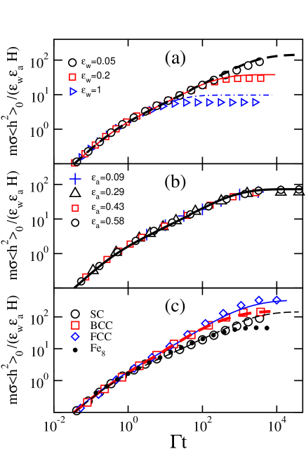
Figure 1: (a) $m\sigma\langle h^{2}\rangle_{0}/(\varepsilon_{w}\varepsilon_{a}H)$ versus $\Gamma t$ for an applied external field $H=1$ and the shown values of $\varepsilon_{w}$. Symbols stand for Monte Carlo results, but dashed, full, and dot–dashed lines stand for results obtained from Eq. (20) for $\varepsilon_{w}=0.05,0.2$, and $1$, respectively. Before field $H$ was applied, thermalization took place from an initially disordered configuration up to the time when the energy $-\varepsilon_{a}$ reached the value $-0.58$. Data points for $\Gamma t<4$ follow from $4\times 10^{4}$ runs for systems of $16\times 16\times 16$ spins on a SC lattice. For $\Gamma t>4$, all data points are for averages over $4\times 10^{5}$ runs of systems of $8\times 8\times 8$ spins in a SC lattice. (b) Same as in (a) but for the shown values of $\varepsilon_{a}$ and $\varepsilon_{w}=0.1$. The continuous line is from the numerical solution of Eq. (20). (c) Same as in (a) and (b), but for different lattices. Symbols stand for MC results. Lines stand for results from theory: dashed is for SC and Fe₈ lattices, dot–dashed and full lines are for BCC and FCC lattices respectively. For SC, BCC, FCC, and Fe₈ lattices, partial thermalization previously took place at $T_{a}=10$, $20$, $60$, and $1.06$K, till $\varepsilon_{a}=0.31$, $0.28$, $0.53$, and $0.15$K, respectively. (For easy comparison with table I, units for Fe₈ are given in Kelvin –but not for cubic lattices.) We used $\varepsilon_{w}=0.05$ for all cubic lattices and $\varepsilon_{w}=11$mK for Fe₈.

The plan of the paper is as follows. The model and Monte Carlo simulations are described in Sect. II. We also explain in Sect. II how we simulate constant energy processes. Section III is devoted to the theory. As an introduction to the rest of the section, qualitative arguments are given in Sec. III.1. The difference between the probability density functions for up–spins and down–spins with a dipolar field $h$ acting on them, which develop during the stage before quenching to very low temperatures, is derived in Sec. III.2. The theory for the magnetization process that takes place after a magnetic field $H$ is applied, soon after quenching, is given in Sec. III.3 and the Appendix. Field functions that are defined below develop in time holes that have been observed experimentallyww1 and are intimately related to the magnetization process. How these holes develop in time is the subject of Sec. III.4. In Sec. III.5, we study the relaxation in zero field of the magnetization of systems that have been previously cooled in weak fields. In Sec. III.6 we show how the magnetization crosses over to a linear in time behavior long after a field is applied if energy exchange between the magnetic system and heat reservoir takes place. Finally, the results obtained are discussed in Sec. IV.

Table 1: $\sqrt{\langle h^{2}\rangle_{0}}$ stands for the rms spatial average of the dipolar field, $\sigma\equiv[\sqrt{2\pi}p(0)]^{-1}$, and $p(0)$ stands for the PDF at $h=0$ on a randomly chosen site, both for completely random spin configurations. Except for Fe₈, they are both in units of $g\mu_{B}Sa^{-3}$, and follow from present MC simualtions; $a$ is the lattice constant for cubic lattices. $T_{0}$ and $\varepsilon_{0}$ stand for the ordering temperature and ground state energy, respectively. Their values are taken from the shown references. $k_{B}T$ and $\varepsilon_{0}$ are, except for Fe₈, in units of $(g\mu_{B}S)^{2}a^{-3}$.

LATTICE	$n_{b}$	$\sqrt{\langle h^{2}\rangle_{0}}$	$\sigma$	$T_{0}$	$\varepsilon_{0}$
SC	1	3.655	3.83(2)	2.50(5)	-2.68(1)
BCC	2	3.864	4.03(2)	5.8(2)	-4.0(1)
FCC	4	8.303	8.44(2)	11.3(3)	-7.5(1)
Fe8	1	46(1) mT	31(1) mT	0.4(1) K	-0.51(2) K

These numbers for $T_{0}$ and $\varepsilon_{0}$ are from Ref. dipole, .
We assume an easy anisotropy axis as given in JF, ; barra, . $T_{0}$ and $\varepsilon_{0}$ are from Ref. erratum, .

II Model and simulation

We use the MC method to simulate magnetic relaxation of Ising systems of $\pm S$ spins, on simple cubic lattices with periodic boundary conditions (PBC), that interact through magnetic dipolar fields and flip under rules to be specified below.Ising In our PBC scheme, two spins interact whether they are in the same box or in different replicated boxes, but a spin at x,y,z interacts with a spin at x’,y’,z’ only if $-L_{x}/2\leq x-x^{\prime}<L_{x}/2$, $-L_{y}/2\leq y-y^{\prime}<L_{y}/2$, and $-L_{z}/2\leq z-z^{\prime}<L_{z}/2$, where $L_{x}$, $L_{y}$, and $L_{z}$ are the sides of the box–like systems we simulate. Thus each spin interacts with $N-1$ spins, where $N$ is the number of spins in the system. This scheme has been tested against a free–boundary scheme,dipole ; Alonso in which all spins in the system are allowed to interact, and found satisfactory when the system is only weakly polarized (or not at all), as is expected from Griffith’s theorem.griff

The system is first allowed to evolve towards thermal equilibrium at some “high” temperature $T_{a}$. We assume $k_{B}T_{a}\gtrsim U/10$, which implies that spin reversals then take place mostly through overbarrier processes. Accordingly, spin flips are then governed by detailed balance rules, and Eq. (1) is not enforced. For reasons that become clear below, we also impose the restriction $T_{a}\gtrsim T_{0}$, where $T_{0}$ is the long-range ordering temperature. One may think of this first process as a waiting stage that the systems may have to undergo in the cooling process, before quenching to a lower temperature where a tunneling experiment (as in Ref. ww1, ) can be later performed.

Let the time when this first stage is ended by quenching to a temperature below roughly $0.1U/(Sk_{B})$ be $t=0$.sangregorio ; ree Accordingly, Eq. (1) is then enforced on all spin flips for $t>0$. As for detailed balance, we then proceed as follows. We may assume (1) that thermalization of a SMM system with the lattice does not take place (i.e., the energy is constant) at very low temperatures, or (2) that heat is readily exchanged with the lattice, as is sometimes the casemetes . In the latter case, we follow the standard procedure. Monte Carlo results illustrate these two cases in Fig. 2. We fulfill the constant energy condition by enforcing detailed balance but using an appropriately chosen pseudotemperature $T_{u}$. [From an expression below Eq. (7), $k_{B}T_{u}\approx\langle h^{2}\rangle_{0}/2\varepsilon_{a}$.xxx Note that $T_{u}\geq T_{a}$, since $-\varepsilon_{a}$ cannot be smaller than the equilibrium energy at $T_{a}$]. We have checked that the mean energy is indeed constant under this rule, as illustrated in Fig. 2. Unless otherwise stated (as in sect. III.6), results reported below are for constant energy processes.

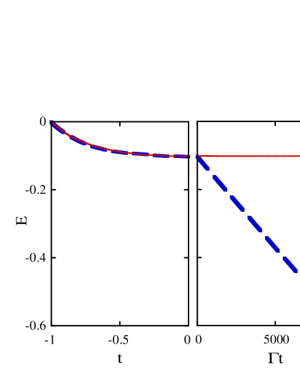
Figure 2: Energy versus time in the annealing stage, when $t<0$, and after quenching, when $t>0$. The time scale in the annealing stage, when $t<0$, is such that the rate for energy lowering spin flips is $1$. In the annealing stage $T=62$ in both cases. For comparison purposes, the ordering temperature $T_{0}$ and the ground state energy $\varepsilon_{0}$ are given in Table I. For $t>0$, the continuous and dashed lines are for constant energy and for an isothermal process at $T=1$, respectively. Equation (1) was enforced for both evolutions, but, as everywhere else, only when $t>0$. The constant energy process was simulated assuming detailed balance with $T_{u}=63$. These data are for systems $16\times 16\times 16$ spins, with $\varepsilon_{w}=0.1$, averaged over $10^{3}$ runs.

MC results for the time evolution of $m\langle h^{2}\rangle_{0}\sigma/(\varepsilon_{w}\varepsilon_{a}H)$, after a field $H=1$ is applied upon quenching, are shown in Fig. 1(a) for various values of $\varepsilon_{w}$. Before quenching, the system was thermalized at $T_{a}=10/k_{B}$ for some time till the energy per spin reached the value $-0.58$. Clearly, $m$ scales with $\varepsilon_{w}$ up to a crossover time of, roughly, $\Gamma^{-1}\sigma^{2}/\varepsilon_{w}^{2}$, where $m$ levels off. Within the time range $1\lesssim\Gamma t\lesssim\sigma^{2}/\varepsilon_{w}^{2}$, $m\propto\sqrt{t}$. Monte Carlo results that show how $m$ scales with $\varepsilon_{a}$ are exhibited in Fig. 1(b) for $\varepsilon_{w}=0.1$. Scaling holds also for the leveling off value $m_{e}$ of $m$. Equations (2-5) are inferred from these graphs, as well as from the theory given below, from which some of the constants are obtained.

III theory

In this section, we try to understand the results of Sect. II and go somewhat beyond.

III.1 Overview

Rough arguments that can serve to introduce the derivations that follow in subsections below are given in this subsection. Before quenching to very low temperatures, the system is for some time at some temperature $T_{a}$ that is above the ordering temperature $T_{0}$. In addition, $k_{B}T_{a}\gtrsim U/10$. Overbarrier relaxation can then take place, and $\tau=\tau_{0}\exp(U/k_{B}T)$ follows from Arrehnius’ law. Consequently, spin flipping readily takes place in the laboratory within a second’s time if $\tau_{0}\lesssim 10^{-5}$ s. Some correlation between spin $s_{i}$ and field $h_{i}$ at each site $i$ can therefore be established, but no long-range order can develop as long as $T_{a}\gtrsim T_{0}$. Thus, immediately after quenching, the joint probability density to find a spin up $p_{\uparrow}(h)$ with a field $h$ acting on it is larger than $p_{\downarrow}(h)$ if $h>0$ and vice versa. This is illustrated in Fig. 3(a). As the system evolves towards equilibrium before quenching, we expect $f(h)\equiv p_{\downarrow}(h)-p_{\uparrow}(h)$ to increase. It is shown in the following section and illustrated in Fig. 3(b) with MC results, that thermalization effects prior to cooling to very low temperatures turn out to be rather simple: $f(h)\propto\varepsilon_{a}hp(h)$ if $\varepsilon_{a}\ll\mid\varepsilon_{0}\mid$, where $p(h)=p_{\uparrow}(h)+p_{\downarrow}(h)$ and $\varepsilon_{0}$ is the ground–state energy ($-2.68$ for a SC lattice). Since $m=-\int dhf(h)$ (from the definition of $f$), $m\propto\varepsilon_{a}$ is expected to ensue after quenching and application of an external field.

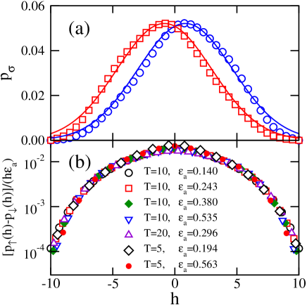
Figure 3: (a) $p_{\sigma}(h)$, versus $h$. All data points are for a system of $16\times 16\times 16$ spins. $\Box$ and $\circ$ stand for down–spin and up–spin, respectively. Full lines are for Gaussian functions centered on $h=0.84$ and $h=-0.84$, with standard deviations of $3.83$. The system was cooled to a temperature $T_{a}=10$, from an infinite temperature, and allowed to evolve towards equilibrium (but not to reach it) till its energy reached the value $-\varepsilon_{a}=-0.42$. For comparison purposes see $T_{0}$ and the ground state energy values in Table I, and the energy is given by $(1/2)\int h[p_{\uparrow}(h)-p_{\downarrow}(h)]dh$ when no external field is applied. All points stand for averages over $1.5\times 10^{5}$ runs. (b) $[p_{\uparrow}(h)-p_{\downarrow}(h)]/(h\varepsilon_{a})$ versus $h$ for the shown values of $\varepsilon_{a}$. No results are shown in the interval $-0.1<h<0.1$, as division by $h$ in the $h\sim 0$ neighborhood enhances errors greatly.

After quenching in the laboratory to a temperature below approximately $0.1U/S$, spin reversals take place only by tunneling between $S_{z}=-S$ and $S_{z}=+S$ states. For this, a spin must be within the “tunnel window” (TW), defined by $\eta$ in Eq. (1). Let some field $H$, fulfilling $H^{2}\ll\langle h^{2}\rangle_{0}$, be applied after quenching. Then, $h+H$ must be within the TW, that is, only spins with a magnetic dipolar field within a TW centered on $h=-H$ can flip. Consider some $H>0$. A look at Fig. 3(a) shows that $p_{\downarrow}(-H)>p_{\uparrow}(-H)$ then, which implies that $m$ must increase with time after $t=0$, since the number of upward flips minus the number of downward flips is proportional to $p_{\downarrow}(h)-p_{\uparrow}(h)$ within the TW (the Zeeman energy for $h=-H$ vanishes and we are assuming $k_{B}T\gg\varepsilon_{w}$). We therefore expect $p_{\downarrow}(h)\rightarrow p_{\uparrow}(h)$ with time if $h$ is within the TW, but both $p_{\downarrow}(h)$ and $p_{\uparrow}(h)$ to remain approximately constant for some time if $h$ is outside the TW. Monte Carlo results illustrate this behavior in Figs. 4(a) and (b). This is much as in the experiments of Wernsdorfer et al.ww1 In addition, inspection of Fig. 3(a) suggests that $f(h)\propto h$ if $h^{2}\ll\langle h^{2}\rangle_{0}$, whence $m\propto H$ also follows. Finally, since the number of spin flips increases linearly with $\varepsilon_{w}$ if $\varepsilon_{w}^{2}\ll\langle h^{2}\rangle_{0}$, we expect $m\propto\varepsilon_{w}$. This is all as in Eq. (2).

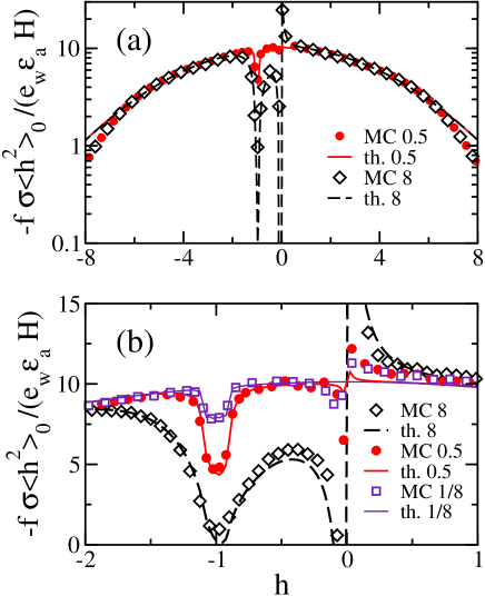
Figure 4: (a) $f\sigma\langle h^{2}\rangle_{0}/(\varepsilon_{a}\varepsilon_{w}h)$, at the shown times, for a system of $16\times 16\times 16$ spins, after it was thermalized at $T=10$ till $\varepsilon_{a}\simeq 0.51$, then abruptly cooled, when $H=1$ was applied. Closed (open) symbols stand for MC (theory) results. A tunnel window $\varepsilon_{w}=0.1$ was enforced. All points stand for averages over $6\times 10^{5}$ histories. (b) Same as in (a) but for the shown values of time. All results obtained from theory for $f(h,t)$, that is, from Eq. (20) were multiplied by $1.27$ in parts (a) and (b). The need for this correction quite likely comes from second order effects in $\varepsilon_{a}/\sigma$ not included in the theory (see Sec. III.2).

The field $h$ acting on a spin does not remain long within the TW after the spin flips. Changing fields produced by other spin flips bring $h$ out of the TW, much as in a random walk. Thus, the “hole” (or “well”) exhibited in Fig. 4(a) widens as in a diffusion process. This is treated in detail in Sec. III.4 and illustrated in Fig. 4(b). Initially, we expect the well’s width $\delta w$ to increase linearly with time, since a dilute, spatially random distribution of spins gives a Lorentzian field distribution,PWA with a width that is proportional to the concentration. However, as the concentration $c$ of flipped spins grows, the corresponding field distribution becomes Gaussian, with $\delta w\propto\sqrt{c}$. Consequently, we expect $m\propto\sqrt{t}$ to ensue after some time since $m\propto-\int dhf(h)$ and this integral grows as $\delta w$ after $f$ nearly vanishes within the TW [see Fig. 4(b)], and remains nearly constant therein subsequently.

The $m\propto\sqrt{t}$ growth stage comes to an end when $\delta w$ becomes as wide as the field distribution over all spins. Then $m$ levels off to $m=m_{s}$. If however the magnetic system can exchange energy with the lattice at very low temperature, then a thermally driven magnetization process eventually takes over. This is the subject of Sec. III.6

III.2 Annealing

Assume that either $T_{a}\gg T_{0}$ or that the time spent in the waiting stage is so short that the PDF that a randomly chosen site have field $h$ is not drastically different from the PDF, $p(h)$, for a totally random spin configuration.gauss On the other hand, the conditional probability to find $\pm S$ on a site where the field is $h$ fulfills, in equilibrium, $p(\pm S\mid h)\propto\exp(\pm h/k_{B}T)$. Now, since the joint distribution $p(\pm S,h)$ for finding, on a randomly chosen site, $h$ and $\pm S$ is in general given by $p(\pm S,h)=p(\pm S\mid h)p(h)$,

$$p(\pm S,h)\propto p(h)e^{\pm h/k_{B}T}$$ (7)

follows in equilibrium. Monte Carlo results illustrate this point in Fig. 3(a). Therefore, since the mean energy is $\langle E\rangle=(1/2)\int dhh[p_{\downarrow}(h)-p_{\uparrow}(h)]$, it follows that $\langle E\rangle\simeq\langle h^{2}\rangle_{0}/2k_{B}T$,xxx where $\langle h^{2}\rangle_{0}\equiv\int dhh^{2}p(h)$. The replacement $\langle h^{2}\rangle_{0}/2k_{B}T\rightarrow\varepsilon_{a}$ generalizes the above equation to

$$p(\pm S,h)\propto p(h)e^{\pm 2h\varepsilon_{a}/\langle h^{2}\rangle_{0}}$$ (8)

for all times up to equilibration. Then, to leading order in $\varepsilon_{a}h/\langle h^{2}\rangle_{0}$,

$$p_{\uparrow}(h)-p_{\downarrow}(h)\simeq 2\frac{h\varepsilon_{a}}{\langle h^{2}\rangle_{0}}p(h),$$ (9)

where $p_{\uparrow}(h)=p(S,h)$ and $p_{\downarrow}(h)=p(-S,h)$. Therefore, for Gaussian field distributions,gauss

$$p_{\uparrow}(h)-p_{\downarrow}(h)\simeq\sqrt{\frac{2}{\pi}}\frac{h\varepsilon_{a}}{\sigma^{3}}e^{-h^{2}/2\sigma^{2}},$$ (10)

since $\langle h^{2}\rangle_{0}=\sigma^{2}$ then. All points for $[p_{\uparrow}(h)-p_{\downarrow}(h)]/(h\varepsilon_{a})$ obtained from MC calculations for SC lattices collapse onto a single curve in Fig. 3(b), in agreement with Eq. (10).

All results given below are for $\varepsilon_{a}/\sigma\lesssim 0.15$. This can be accomplished by annealing at $T\gtrsim 4T_{0}$. In addition, only applied fields much smaller than $\sigma$ are used. Thus, significant higher–order (in $\varepsilon_{a}h/\sigma^{2}$) contributions are avoided.

Note that Eqs. (7)–(10) are valid only in the annealing stage. They are inapplicable after quenching, because spins are then not free to adjust to local fields.

III.3 Magnetization process

We now examine the system’s time evolution after cooling it abruptly, at time $t=0$, to a temperature below, roughly, $0.1U/(Sk_{B})$. A field $H$ is applied for all $t>0$. Then, real spin flips up to $\mid S_{z}\mid<\,S$ states can be neglected, and tunneling through the ground state doublet is the only available path for spin reversals. Accordingly, spin flips are allowed only if the spin’s Zeeman energy is within the tunnel window. Now, if either the system is in thermal contact with a reservoir at temperature $T$ such that $k_{B}T\gg\varepsilon_{w}$, or the energy is constant and sufficiently high such that $k_{B}T_{u}\gg\varepsilon_{w}$, then

$$\dot{m}(t)=2\Gamma\int dh\,\eta(H+h)f(h;t),$$ (11)

where $f(h;t)\equiv p_{\downarrow}(h;t)-p_{\uparrow}(h;t)$. Let

$$\dot{\mu}(h,H;t)\equiv 2\Gamma\,\eta(H+h)f(h;t),$$ (12)

whose physical meaning follows from comparison of these two equations.

It is important to note that, Eq. (12) notwithstanding, $\dot{\mu}\neq-\dot{f}$. This is because $\dot{\mu}$ has to do with numbers of spin flips, not with changes in dipolar fields, which are brought about by such spin flips and also contribute to $\dot{f}$. In order to establish how $f$ evolves with time, it is convenient to define $g(h;t)\equiv f(h,0)-f(h;t)$. Now, $g(h;t)$ changes because spins which flip on sites where the field is within $h$ and $h+dh$ contribute $\dot{\mu}(h,H;t)\Delta tdh$ to $gdh$ in time $\Delta t$, and also because of dipolar field changes brought about by such flips. These two effects are approximately taken into account in,

$$g(h;t)\simeq\int_{0}^{t}d\tau\int d\tilde{h}G(h,\tilde{h};t-\tau)\dot{\mu}(\tilde{h},H,\tau),$$ (13)

where $G(h,\tilde{h};t-\tau)$ is the PDF that, on a randomly chosen site, the field is $h$ at time $t$, given that the field on that site was $\tilde{h}$ at time $\tau$. Again, note that $\dot{f}=-\dot{\mu}$ would only follow if field redistributions, owing to spin flips, were disregarded, that is, if $G(h,\tilde{h};t-\tau)$ were replaced by $\delta(h-\tilde{h})$ in Eq. (13).

We next approximate $G(h,\tilde{h};t-\tau)$. Recall that $H^{2}\ll\langle h^{2}\rangle_{0}$ throughout. Consider a spin that points in opposite directions at times $t$ and $\tau$. Let the fractional number of all such spins be $\phi(t,\tau)$. Since $p(h,t)$ is approximately constant for the times of interest here, $\phi(t,\tau)\simeq\phi(t-\tau)$. For $\phi(t-\tau)\ll 1$, we expectPWA

$$G(h,\tilde{h};t-\tau)\simeq\frac{u(t-\tau)}{\pi[(h-\tilde{h})^{2}+u(t-\tau)^{2}]},$$ (14)

where $u=2h_{0}\phi$, $h_{0}=(8\pi^{2}/3^{5/2})g\mu_{B}S\rho_{v}$, $\rho_{v}$ is the number of spin sites per unit volume. Near the other end of the time range, when $\phi(t-\tau)\rightarrow 1/2$, we letgauss

$$G(h,\tilde{h};t-\tau)\simeq\frac{e^{-(h-\tilde{h})^{2}/(2v^{2})}}{\sqrt{2\pi}v(t-\tau)},$$ (15)

where $v=\sigma\sqrt{2\phi(t-\tau)}$, when $\phi(t-\tau)\rightarrow 1/2$.

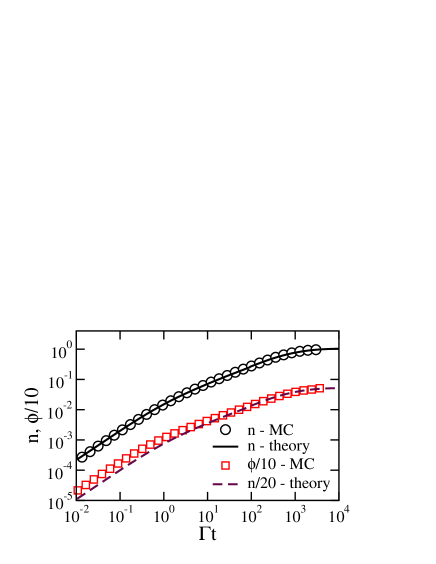
Figure 5: Fraction of all spins $n$ that have flipped at least once, and quantity $\phi/10$ versus $\Gamma t$. In order to avoid cluttering, $\phi/10$, instead of $\phi$ is plotted. All results are for $\varepsilon_{w}=0.1$. $\circ$ and $\Box$ stand for MC averages over $5\times 10^{4}$ evolutions; the continuous and dashed lines follow numerically from Eq. (20). $n/20$ should equal $\phi/10$, according to Eq. (17).

To make progress, $\phi(t-\tau)$ must now be determined. Let $\rho(h;t)$ be the PDF that a spin with a field $h$ acting on it has flipped at least once in time $t$. In order to relate $\phi$ and $n$, given by

$$n(t)=\int dh\,\rho(h;t),$$ (16)

we note that the total number of spin flips is much larger than the number of first time flips at all times. This implies that spins flip several times before the dipolar field acting on them drifts away from the tunnel window. Accordingly, (see Fig. 5) we adopt

$$\phi=n/2.$$ (17)

Finally, we write an equation for $\rho(h;t)$, from which $n(t)$ and, consequently, $\phi(t)$ then follow. Arguing as for Eq. (13),

$$\rho(h;t)\simeq\int_{0}^{t}d\tau\int d\tilde{h}G(h-\tilde{h};t-\tau)\dot{\nu}(\tilde{h},H,\tau),$$ (18)

follows, where

$$\dot{\nu}(h,H,\tau)\equiv[p(h,0)-\rho(h,\tau)]\eta(h+H),$$ (19)

and we have assumed once again that $p(h;t)=p(h,0)$.

The desired equation for the magnetization process,

$$\frac{dx}{dt}\simeq c_{1}\frac{p(-H)}{p(0)}-c_{2}\int^{t}_{0}d\tau\frac{dx}{d\tau}\frac{2\varepsilon_{w}}{\omega(H;t-\tau)+2\varepsilon_{w}},$$ (20)

where $x=m\sigma\langle h^{2}\rangle_{0}/(\varepsilon_{a}\varepsilon_{w}H)$, $c_{1}=4\sqrt{2/\pi}$, $c_{2}=2$, and $\omega(H;t-\tau)\equiv 1/G(-H,-H;t-\tau)$, is derived in the Appendix. The above equation also holds for $n(t)$ if we let $x=n\sigma/\varepsilon_{w}$, $c_{1}=\sqrt{2/\pi}$ and $c_{2}=1$.

For $H^{2}\ll\langle h^{2}\rangle_{0}$ and $H\ll h_{0}$,mT $\omega(-H;t-\tau)\rightarrow u(t-\tau)$ in Eq. (14) and $\omega(-H;t-\tau)\rightarrow\sqrt{2\pi}v(t-\tau)$ in Eq. (15). Then,

$$\omega\simeq\min[2\pi h_{0}\phi,\sigma\sqrt{4\pi\phi}]$$ (21)

is an approximation that fits data obtained from simulations of field distributions from various concentrations, $2\phi$, of randomly placed spins, in an otherwise empty lattice, reasonably well. In Eq. (21), $\omega$ depends on $t-\tau$ through $\phi$ and, consequently, through $n$.

The functional dependence of $F$, shown in Eq. (2), follows from Eqs (20) and (21). To see how Eq. (3) comes about, notice first that $\omega\ll\varepsilon_{w}$ when $\Gamma t\ll 1$. Then, Eq. (20) becomes $dx/d(\Gamma t)\simeq c_{1}-c_{2}x$ for $H^{2}\ll\langle h^{2}\rangle_{0}$, whence Eq. (3) follows. For Eq. (4), we turn to numerical solutions of Eq. (20) which are exhibited in Figs. 1(a), (b), and (c).

We can obtain an analytic expression for $p$ from Eq. (20). Since numerical solutions of Eqs. (20) and (21) give $x(t)\propto t^{p}$ for $\Gamma t\gtrsim 1$ and vanishingly small $\varepsilon_{w}/\sigma$, we let $\varepsilon_{w}/\sigma\rightarrow 0$ and try $m\propto t^{p}$ as a solution for all $t\gg\Gamma^{-1}$. Equations (17) and (21) give

$$\omega\rightarrow\pi h_{0}n$$ (22)

as $\varepsilon_{w}/\sigma\rightarrow 0$. Consider first $x=n\sigma/\epsilon_{w}$, and, consequently, $c_{1}=\sqrt{2/\pi}$ and $c_{2}=1$. Then, for $H\ll\sigma$, Eq. (20) becomes

$$\frac{dx}{dt}\simeq\sqrt{\frac{2}{\pi}}-\int^{t}_{0}d\tau\frac{dx(\tau)}{d\tau}\frac{1}{\alpha x(t-\tau)+1},$$ (23)

where $\alpha=\pi h_{0}/(2\sigma)$. Assuming $x\sim t^{p}$, the change of variable $z=\tau/t$, brings Eq. (23), in the $t\rightarrow\infty$ limit, to

$$0=\sqrt{\frac{2}{\pi}}-\int^{1}_{0}dz.\frac{pz^{p-1}}{\alpha(1-z)^{p}},$$ (24)

Equation (6) follows immediately from integral tables grads . We now return to Eq. (20) to work with $x=m\sigma\langle h^{2}\rangle_{0}/(\varepsilon_{a}\varepsilon_{w}H)$, $c_{1}=4\sqrt{2/\pi}$, and $c_{2}=2$. We now assume $x\sim t^{\tilde{p}}$, and, proceeding as above, obtain (1) $\tilde{p}=p$ and (2) $m/n\rightarrow 2\varepsilon_{a}H/\langle h^{2}\rangle_{0}$ as $t\rightarrow\infty$. Therefore, $p$ in $m\propto t^{p}$ is given by Eq. (6).

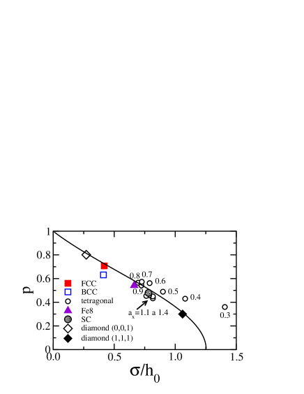
Figure 6: Quantity $p$, defined by $m\propto t^{p}$, versus $\sigma/h_{0}$. Symbols stand for MC results for the shown lattices for $\varepsilon_{w}=0.05$ and $H\lesssim\sigma/4$. The lattice structure for Fe₈ is as in Ref. Fe_8, . The numbers next to symbols for the tetragonal lattice stand for the ratio of the basal to the $z$–axis lattice constant. (0,0,1) and (1,1,1) stand for easy magnetization axes. The full line stands for Eq. (6).

Quantity $p$ from Eq. (6), as well as results for $p$ obtained from MC simulations for various lattices, are exhibited in Fig. 6. Monte Carlo generated data points are in reasonably good agreement with theory, that is, with Eq. (6), except for tetragonal lattices with $0.3$ and $0.4$ ratios of the basal to the $z$–axis lattice constant (i.e., for $\sigma/h_{0}\simeq 1.08$ and $1.42$, respectively). This departure may follow from the fact that, for these rather asymmetric lattices, $1/p(h=0)$ turns out to be nonlinear in the concentration $n$ of spin occupied lattice sites for $n\gtrsim 0.01$. This is in contradiction with Lorentzian field distributionsPWA we have assumed for $n\ll 1$. Such distributions give $p(h=0)\propto n^{-1}$, which comes into Eq. (20) through Eq. (21).

The relation $m/n\rightarrow 2\varepsilon_{a}H/\langle h^{2}\rangle_{0}$ holds just as well for small but finite $\varepsilon_{w}/\sigma$, whence the constant $(1/2)\sqrt{\pi/2}$ in Eq. (5) follows, since $n\rightarrow 1$ as $t\rightarrow\infty$. In addition, an intuitive argument that gives some insight into Eq. (5) is given in Sect. III.6.

III.4 Tunnel window’s imprint and field diffusion

It is interesting to see how $g(h;t)$ behaves for early times, when $u\ll\varepsilon_{w}$ and $\phi\ll 1$. It then follows from Eq. (14) that $G(h)$ can be replaced by $\delta(h+H)$ in Eq. (13), which in turn yields

$$\dot{g}(h,H;t)=2\Gamma\eta(h+H)[f(h,0)-g(h;t)],$$ (25)

and, consequently, for $\Gamma t\ll 1$,

$${g}(h;t)=f(h,0)\eta(h+H)(1-e^{-2\Gamma t}).$$ (26)

Therefore, when the variation of $f(h,0)$ over $\eta(h+H)$ is negligible, $g(h;t)$ is the tunnel window’s imprint. This is illustrated in Fig. 4(b). A conjecture to this effect was made in Ref. ww1, . In order to show how long the condition $u\ll\varepsilon_{w}$, necessary for the validity of Eq. (26), holds, note that the total number of spins that flip in time $t$ is approximately $p(h;0)\varepsilon_{w}\Gamma t$. It follows immediately that $u\ll\varepsilon_{w}$ if $\Gamma t\ll\sigma/h_{0}$. Therefore, Eq. (26) holds while $\Gamma t\ll 1$.hole3 This is illustrated in Fig. 4(b). Monte Carlo results for exponential TW shapes that further illustrate this behavior are reported in Ref. JMMM, .

After $\Gamma t\sim 1$, $g(h;t)$ no longer grows as in Eq. (26), with constant width. When $\Gamma t\gg 1$, the width of $g(h;t)$ grows with time. A spin flip at any one site induces variations of dipolar fields at every other site. Wherever a spin flipped at time $\tau$ the field $h$ evolves as in a random walk, away from $h=-H$ at time $\tau$, and $G(h,-H;t-\tau)$ is its distribution at time $t$, as given in Eq. (14) while $\phi(t-\tau)\ll 1$. In this sense, one may then speak of dipole field diffusion. It is the purpose of this section to calculate such field diffusion. A Fourier transformation of Eq. (35) gives

$$g(k;t)\simeq\int_{0}^{t}d\tau G(k;t-\tau)\eta(bk)\frac{\dot{m}(\tau)}{2\varepsilon_{w}},$$ (27)

where $g(k;t)=\int dh\exp(-ikh)g(h;t)$, $G(k;t)=\int dh\exp[-ik(h-b\tilde{h})]G(h,\tilde{h};t)$, $\eta(bk)=\int dh\exp[-ibk(h+H)]\eta(h+H)$, and $b=1-2\phi(t-\tau)$. A similar equation [letting $g(k;t)\rightarrow\rho(k;t)$ and $m(\tau)\rightarrow n(t)$ in Eq. (27)] obtains for $\rho(k;t)$. Equation (27) can be solved numerically with the help of Eqs. (14)–(21). Results obtained are shown in Figs. 4(a) and (b). Perhaps it is worth pointing out that $p(h)$ changes appreciably only after very long times when strong spin–spin correlations develop as the equilibrium ordered state is approached.Alonso ; JMMM

The spike in $f/h$, which develops at $h=0$ after some time, was not observed experimentally.ww1 However, it is not a spurious effect. It is a consequence of the fact that the hole in $f$ spreads out in time, which implies that $f(0,t)<0$ when $t>0$. The spike in $f/h$ at $h=0$ has a physical consequence: if $H$ is switched off at some time $t\gtrsim 1$, a hole in $f(h,t)$ will develop at $h=0$, and the magnetization will decrease in time accordingly.differ

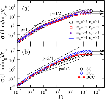
Figure 7: (a) $\sigma(1-m/m_{0})/\varepsilon_{w}$ versus $\Gamma t$ for zero field relaxation from weakly polarized states for the shown values of $\varepsilon_{w}$ and of $m_{0}$. Data points for $\Gamma t<64$ (for $64<\Gamma t<4\times 10^{4}$) follow from averages over $10^{5}$ (some $2\times 10^{4}$) MC simulations of systems of $16\times 16\times 16$ ($8\times 8\times 8$) spins. (b) Same as in (a) but for BCC and FCC lattices, $\varepsilon_{w}=0.1$ and $m_{0}=0.2$. The points indicated by the horizontal arrows correspond to $m\rightarrow 0$. The sloping lines for $t^{p}$, for the shown values of $p$, are given for comparison purposes.

III.5 Relaxation in zero field

A slight variation of the experiment above is considered in this section. Suppose a magnetic field $H$ is applied during the annealing stage, so that a polarization develops before quenching to very low temperatures, and let this applied field be switched off at $t=0$, soon after quenching. Note that this differs from the problem considered in Refs. PS, and vill, of systems that are initially fully polarized. Now, for a weakly polarized system, we expect

$$p_{\uparrow}(h;0)\simeq\frac{1}{2}(1+m_{0})p(h;0),$$ (28)

where $m_{0}$ is the initial magnetization, and similarly for $p_{\downarrow}(h;0)$ letting $m_{0}\rightarrow-m_{0}$. For $H\ll 1$,

$$f(H,0)\simeq-\frac{m_{0}}{\sqrt{2\pi}\sigma},$$ (29)

follows. Now, formally, replacement of $\varepsilon_{a}h/\langle h^{2}\rangle_{0}$ by $-m_{0}/2$ in Eq. (9) gives the equation above. Since everything else works for the relaxation of the magnetization the same as in Sec. III.3, substitution of $\varepsilon_{a}h/\langle h^{2}\rangle_{0}$ by $-m_{0}/2$ in Eq. (2) leads to

$$m\simeq m_{0}[1-b^{\prime}\varepsilon_{w}\sigma^{-1}F(\Gamma t,\sigma/\varepsilon_{w},\sigma/h_{0})],$$ (30)

where $b^{\prime}=2\sqrt{2/\pi}$ and $F$ is given by Eqs. (3)-(5). This is the desired equation. Consequently, $m$ becomes vanishingly small after $\Gamma t\simeq(\sigma/\varepsilon_{w})^{1/p}$. As in sections above, $p\simeq 0.5$ for SC lattices, but is different for other lattices. Up to then, $m$ relaxes, after $\Gamma t\approx 1$, as $t^{p}$. Monte Carlo results illustrating this behavior are shown in Figs. 7(a) and (b).

Thus, systems that are weakly polarized at quenching relax afterwards in complete analogy to the magnetization process described in previous sections. Relaxation proceeds as $t^{p}$, from $\Gamma t\sim 1$ up to the time $(\sigma/\varepsilon_{w})^{1/p}$, when $m$ reaches a vanishingly small value. In addition, quantity $p$ depends on lattice structure the same as above and as in Fig. 6. This differs fundamentally from the relaxation of systems that are initially fully polarized, which are the subject of Refs. PS, and exp, ; expb, ; vill, . In the latter condition: (1) the relaxation of the magnetization depends crucially on system shape;C (2) a $\sqrt{t}$ relaxation is predicted to be independent of lattice structure; (3) this behavior holds whilePS ; exp $\varepsilon_{w}/\sigma\lesssim\Gamma t$ and $m\gtrsim 0.9m_{s}$, which take place much earlier than the magnetization processes that are the subject of this paper.

III.6 Late time magnetization

If the magnetic system does not exchange energy with the lattice, the magnetization finally levels off to the stationary value $m_{s}\simeq 1.6\varepsilon_{a}H/\langle h^{2}\rangle_{0}$, given by Eqs. (2) and (5). To gain some insight into this, note that: (1) $m=\int dhg(h)$; (2) $g(h,t)$ comes near its stationary value, $f(-H,0)$, in the vicinity of $h=-H$ when $\Gamma t\gtrsim 1$; afterwards, (3) $\int dhg(h,t)$ increases with time mostly because the width $\delta w$ of $g(h,t)$ increases up to the time when $\delta w\approx 2\sqrt{\langle h^{2}\rangle_{0}}$, that is, when $g(h,t)$ becomes as wide as $p(h)$, and reaches its stationary state. Then, $\int dhg(h)\approx f(-H,0)2\sqrt{\langle h^{2}\rangle_{0}}$, which, making use of Eq. (9) for $f(-H,0)$ with $\mid H\mid\ll 1$, and of $\sigma^{2}\sim\langle h^{2}\rangle_{0}$, gives the desired estimate for $m_{s}$. This comes to be when all spins have flipped at least once, i.e., when $n(t)\rightarrow 1$. The time evolution of $n(t)$ is shown in Fig. 5 for $\varepsilon_{w}=0.1$.

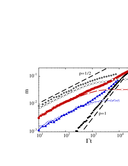
Figure 8: $m$ versus $\Gamma t$ for $\varepsilon_{w}=0.1$, and $H=1$. All data points are for MC simulations of $16\times 16\times 16$ spin systems. Open (full) symbols stand for evolutions in which heat exchange between magnetic and lattice systems does not (does) take place. $\bullet$ is for $\varepsilon_{a}=0$, $\triangle$ is for $\varepsilon_{a}=0.10$, $\blacktriangle$ is for $\varepsilon_{a}=0.097$, $\Box$ is for $\varepsilon_{a}=0.29$, $\blacksquare$ is for $\varepsilon_{a}=0.29$, $\Diamond$ is for $\varepsilon_{a}=0.58$, and $\blacklozenge$ is for $\varepsilon_{a}=0.58$. Data points stand for averages over at least $10^{3}$ MC runs. For comparison purposes, two straight dashed lines for $m\propto t^{p}$ are shown.

On the other hand, even when $k_{B}T\lesssim 0.1U/S$, heat exchange between magnetic and lattice systems does take place in some systems of SMM’s.metes Then, the magnetization can increase further with time as the system evolves towards its thermal equilibrium state. As has previously been shown,Ising a relaxation time $\tau_{th}$ can then be defined, which is given by

$$\Gamma\tau_{th}\approx\left(\frac{\sigma}{\varepsilon_{w}}\right)^{3}.$$ (31)

Accordingly, we expect

$$m(t)\simeq c\frac{H}{\sigma}\frac{t}{\tau_{th}}$$ (32)

to hold when thermalization effects become dominant. Equation (32), with $c\simeq 1.5$, gives a rough fit of the nearly linear in time pieces in Fig. (8). A crossover to this late time regime, which is driven by energy exchange with the lattice is easily appreciated in Fig. (8). The corresponding crossover time $\tau_{co}$ is best expressed in terms of another crossover time, $\tau_{s}$, when $m\propto\sqrt{t}$ crosses over to $m=m_{s}$. $\tau_{co}$ follows from Eqs. (1)-(5) and Eq. (32). For $\varepsilon_{a}\gg\varepsilon_{w}$, the thermally driven linear behavior appears after $m$ levels off at $m_{s}$. Letting $\sigma^{2}\sim\langle h^{2}\rangle_{0}$ and $p\approx 2$,

$$\frac{\tau_{co}}{\tau_{s}}\sim\frac{\varepsilon_{a}}{\varepsilon_{w}}.$$ (33)

obtains. On the other hand, if $\varepsilon_{a}\ll\varepsilon_{w}$, linear behavior appears early, and magnetization leveling off is preempted. By the same approximations,

$$\frac{\tau_{co}}{\tau_{s}}\sim\left(\frac{\varepsilon_{a}}{\varepsilon_{w}}\right)^{2},$$ (34)

then follows.

Even later yet, when $t\gtrsim\tau_{th}$, the magnetization crosses over to another regime as long–range order sets in. This can be appreciated in Fig. 8 for $\Gamma t\gtrsim 10^{4}$.

IV conclusions

We have given MC and theoretical evidence to show that the $m\propto\sqrt{t}$ behavior observed in experiments on Fe₈ crystals ww1 after quenching and applying a small field $H$ at $t=0$ is driven by correlations, which are previously established in the system while cooling to very low temperatures. Of the cooling protocol, only the correlation energy $-\varepsilon_{a}$ at the time of quenching matters. The whole magnetization process is ruled by Eqs. (2)-(5) when the magnetic system is thermally isolated.

The $m\propto\sqrt{t}$ behavior has been shown to be nonuniversal. Both MC and theory show that this behavior ensues in SC lattices. Our MC simulations of an Fe₈ model, in the appropriate lattice,erratum give $m\propto\sqrt{t}$, in agreement with experiment.ww1 However, MC simulations of FCC and BCC lattice systems give $m\propto t^{p}$, where $p$ varies with lattice structure as illustrated in Fig. 1(c). Numerical solutions of Eq. (20) show that $p$ depends on lattice structure through $\sigma/h_{0}$ ($h_{0}$, which is defined below Eq. (5), is proportional to the number of spin sites per unit volume) as shown in Fig. 6. Values of $\sigma$ and $p(0)$ are given in Table I for a few lattices. The $m\propto t^{p}$ regime has been shown to cover the time range $1\lesssim\Gamma t\lesssim(\sigma/\varepsilon_{w})^{1/p}$.

Similar results, namely Eq. (30), have been obtained for the magnetization relaxation in zero field of systems that have been previously cooled in weak fields. This differs from the relaxation of fully polarized initial states, where the $1-m\propto\sqrt{t}$ behavior has been shown to be universal for $1-m\lesssim 0.1$.PS More remarkably, our results differ qualitatively from the exponential relaxation predicted in Ref. PS, for weak field cooled systems.

In order to test for system shape, size, and boundary effects, we have also performed MC simulations on spherical and box like systems of various sizes, with periodic and with free boundary conditions on SC lattices. Quantity $p$ for box like systems with PBC appears to be size and shape independent as long as there are more than four spins on each side. Box like systems of $L_{x}\times L_{x}\times L_{z}$ spins with free boundary conditions give values of $p$ that appear to agree in the $L_{x}\rightarrow\infty$ limit if $L_{z}\geq 16$ as well as in the $L_{z}\rightarrow\infty$ limit if $L_{x}\geq 8$. Results for spheres with free boundary conditions also go to the same macroscopic limit : $p=0.49\pm 0.01$ for SC lattices.

The magnetization process depends significantly on whether the magnetic system is thermally isolated or not only after some crossover time $\tau_{co}$, given by Eqs. (33) and (34). This is illustrated in Fig. 8. It might be interesting to observe this effect on systems in which specific heat experiments have shown that energy is exchanged with the lattice within reasonable times at low temperatures.metes

The simple result of Sec. III.4 deserves a comment. It shows that experimentally observed holes in $f(h,t)$ can be used to establish the value of $\Gamma$, since holes develop independently of $\varepsilon_{w}$ and of $\varepsilon_{a}$ while $\Gamma t\lesssim 0.5$, i.e., while $f$ at the bottom of the hole is approximately larger than one half its value at the top. This is useful because there is no other simple relation we know of that one can use in order to extract the value of $\Gamma$ from othe experimental observations. For instance, application of Eq. (26) to Fig. 4 in Ref. ww1, yields $\Gamma^{-1}\simeq 24$ s for Fe₈.

Except for the $m\propto\sqrt{t}$ behavior, which has been observed in Fe₈ over a limited time range,ww1 , all the predictions we make here have yet to be observed experimentally. Since time scales can be controlled, varying $\Gamma$, through the application of a transverse field, experimental observation seems feasible.

Appendix A

Equation (13) can be further simplified making use of the approximation $\dot{\mu}(\tilde{h},H,\tau)\simeq\eta(h+H)\dot{m}(\tau)/2\varepsilon_{w}$. Then,

$$g(h;t)\simeq\int_{0}^{t}d\tau\frac{\dot{m}(\tau)}{2\varepsilon_{w}}\int d\tilde{h}\,G(h,\tilde{h};t-\tau)\eta(\tilde{h}+H)$$ (35)

A similar equation follows for $\rho(t)$, making the replacement ${\nu}(\tilde{h},H,\tau)\rightarrow\eta(h+H)n(\tau)/2\varepsilon_{w}$ in Eq. (18). Now, from Eq. (11) and the definition of $g$,

$$\dot{m}\simeq 2\Gamma\int dh[f(h,0)-g(h;t)]\eta(h+H),$$ (36)

follows immediately, and, similarly for $\dot{n}(t)$ (letting $m\rightarrow n$, $f\rightarrow p$, and $g\rightarrow\rho$ above). Substitution of Eq. (35), into Eq. (36), gives

$$\dot{m}\simeq 2\Gamma\left[2\varepsilon_{w}f(-H,0)-\int_{0}^{t}d\tau\frac{\dot{m}(\tau)}{2\varepsilon_{w}}W(t-\tau)\right],$$ (37)

where $\varepsilon_{w}\ll\sigma$ has been assumed, and

$$W\equiv\int dh\int d\tilde{h}\eta(h+H)G(h,\tilde{h};t-\tau)\eta(\tilde{h}+H).$$ (38)

Approximations on $W$ follow. First, $\Gamma(t-\tau)\ll 1\Longrightarrow u(t-\tau)\ll\varepsilon_{w}$, since $u=2h_{0}\phi$, $n/2\leq\phi\leq n(1-n/2)$, and $n(t)\sim(\varepsilon_{w}/\sigma)\Gamma t$ if $\Gamma t\ll 1$, whence $G(h,\tilde{h};t-\tau)\rightarrow\delta(h-\tilde{h})$, and therefore

$$W\rightarrow 2\varepsilon_{w}$$ (39)

then. By the same argument, $\Gamma(t-\tau)\gg 1\Longrightarrow u(t-\tau)\gg\varepsilon_{w}$, whence it follows that variations of $G$ over the tunnel window are then negligible (from the assumption that $\varepsilon_{w}\ll\sigma$), and

$$W\rightarrow(2\varepsilon_{w})^{2}G(-H,-H;t-\tau)$$ (40)

therefore. We now use

$${W(t-\tau)}\simeq\frac{2\varepsilon_{w}}{[2\varepsilon_{w}G(-H,-H;t-\tau)]^{-1}+1}$$ (41)

to interpolate between Eqs (39) and (40). Substituting this equation into Eq. (37) [and into the analogous equation for $n(t)$] gives Eq. (20), which is the desired equation.

References

- (1) See, for instance, D. Ruiz Molina, G. Christou, and D. N. Hendrickson, Mol. Cryst. Liq. Cryst. 343, 335 (2000).
- (2) J. R. Friedman, M. P. Sarachik, J. Tejada, and R. Ziolo, Phys. Rev. Lett. 76, 3830 (1996); L. Thomas, F. Lionti, R. Ballou, D. Gatteschi, R. Sessoli, and B. Barbara, Nature (London) 383, 145 (1996); J. M. Hernández, X. X. Zhang, F. Luis, J. Bartolomé, J. Tejada, and R. Ziolo, Europhys. Lett. 35, 301 (1996); see also J. A. A. J. Perenboom, J. S. Brooks, S. Hill, T. Hathaway and N. S. Dalal, Phys. Rev. B 58, 330 (1998).
- (3) C. Sangregorio, T. Ohm, C. Paulsen, R. Sessoli, and D. Gatteschi, Phys. Rev. Lett. 78, 4645 (1997).
- (4) For Fe8, see W. Wernsdorfer and R. Sessoli, Science 284, 133 (1999); for Mn12, see F. Luis, J. Bartolomé, and J. F. Fernández, Phys. Rev. B 57, 505, (1998).
- (5) N. V. Prokof’ev and P. C. E. Stamp, Phys. Rev. Lett. 80, 5794 (1998); Rep. Prog. Phys. 63, 669 (2000).
- (6) D. A. Garanin, E. M. Chudnovsky, and R. Schilling, Phys. Rev. B 61, 12 204 (2000); D. A. Garanin and E. M. Chudnovsky, ibid 65, 094423 (2002); R. Amigó, E. del Barco, Ll. Casas, E. Molins, J. Tejada, I. B. Rutel, B. Mommouton, N. Dalal, and J. Brooks, ibid 65, 172403 (2002); see also, A. Cornia, R. Sessoli, L. Sorace, D. Gatteschi, and A. L. Barra, Phys. Rev. Lett. 89, 257201 (2002); E. del Barco, A. D. Kent, E.M. Rumberger, D. N. Hendrickson, and G. Christou, ibid 91, 047203 (2003).
- (7) In Fe8, T. Ohm, C. Sangregorio, and C. Paulsen, Eur. Phys. J. B 6, 195 (1998).
- (8) In Mn12, L. Thomas and B. Barbara, J. Low Temp. Phys. 113, 1055 (1998); L. Thomas, A. Caneschi, and B. Barbara, Phys. Rev. Lett. 83, 2398 (1999); B. Barbara, I. Chiorescu, B. Giraud, A. G. M. Jansen, and A. Caneschi, J. Phys. Soc. Jpn., Suppl. A 69, 383 (2000).
- (9) A. Cuccoli, A. Rettori, E. Adam, and J. Villain, Euro. Phys. J. B 12, 39 (1999).
- (10) E. M. Chudnovsky, Phys. Rev. Lett. 84, 5676 (2000); N. V. Prokof’ev and P. C. E. Stamp, Phys. Rev. Lett. 84, 5677 (2000); W. Wernsdorfer, C. Paulsen, and R. Sessoli, ibid 84, 5678 (2000).
- (11) W. Wernsdorfer, T. Ohm, C. Sangregorio, R. Sessoli, D. Mailly, and C. Paulsen, Phys. Rev. Lett. 82, 3903 (1999).
- (12) J. F. Fernández and J. J. Alonso, Phys. Rev. Lett. 91, 047202 (2003).
- (13) For Gaussian distributions . Numbers we have obtained from MC simulations for and for are listed in Table I.
- (14) For further details about an Ising model of spins that interact through magnetic dipolar fields, and why it is an appropriate model to use for SMM’s at very low temperatures if spin flip rules that include Eq. (1) are enforced, see J. F. Fernández, Phys. Rev. B 66 064423 (2002).
- (15) J. F. Fernández and J. J. Alonso, Phys. Rev. B 62, 53 (2000).
- (16) J. J. Alonso and J. F. Fernández, Phys. Rev. Lett. 87, 097205 (2001).
- (17) The thermodynamic limit of a system of interacting magnetic dipoles is independent of boundary conditions and of system shape if no external field is applied, R. B. Griffiths, Phys. Rev. 176, 655 (1968).
- (18) L. Bokacheva, Andrew D. Kent, and M. A. Walters, Phys. Rev. Lett. 85, 4803 (2000).
- (19) M. Evangelisti, F. Luis, F. L. Mettes, N. Aliaga, G. Aromí, G. Christou, and L. J. de Jongh, Polyhedron 22, 2169 (2003).
- (20) This is also the leading term in a high temperature, , series expansion for the energy, . Hence the energy remains (on the average) equal to in a simulation at temperature .
- (21) A. Abragam, Principles of Nuclear Magnetism (Oxford Science Publications, Oxford, 1996). pp-125-128. A factor of comes in the expressions for , because an spin flip contributes as much as adding a spin to an empty site.
- (22) For some lattices, such as cubic ones, is nearly gaussian. It is not so for the Fe8 lattice, nor for lattices in which sites along the easy magnetization axis are much more closely spaced than sites in other directions.
- (23) A.-L. Barra, D. Gatteschi, and R. Sessoli, Chem.-Eur. J. 6, 1608 (2000); J. F. Fernández and J. J. Alonso, Phys. Rev. B 65, 189901(E) (2002).
- (24) For SMM’s, such as Fe8 and Mn12, mT and mT.
- (25) I. S. Gradshteyn and I. M. Ryzhik Table of Integrals, Series, and Products, fifth edition, edited by A. Jeffrey (Academic Press, N. Y., 1994) p339.
- (26) A “hole” in that resembles was shown in Ref. Alonso, to develop at much later times.
- (27) J. J. Alonso and J. F. Fernández, J. Mag. Mag. Mat. xx, xxxxx (2004).
- (28) Actually, the data plotted in Ref. 11 is not quite the same as [W. Wernsdorfer (private communication)], which may explain why no hole was seen experimentally.
- (29) See Prokof’ev and Stamp in Refs. PS, and comm, .
- (30) J. F. Fernández and J. J. Alonso, Phys. Rev. B 65, 189901 (2002).
- (31) T. Ohm, PhD thesis (Grenoble), Joseph Fourier University (1998).
- (32) A.-L. Barra, D. Gatteschi, and R. Sessoli, Chem.-Eur. J. 6, 1608 (2000).