Electron–phonon interaction effects in semiconductor quantum dots: a non-perturbative approach

Abstract

Multiphonon processes in a model quantum dot (QD) containing two electronic states and several optical phonon modes are considered taking into account both intra- and inter-level terms. The Hamiltonian is exactly diagonalized including a finite number of multi-phonon processes, large enough as to guarantee that the result can be considered exact in the physically important region of energies. The physical properties are studied by calculating the electronic Green’s function and the QD dielectric function. When both the intra- and inter-level interactions are included, the calculated spectra allow for explanation of several previously published experimental results obtained for spherical and self-assembled QDs, such as enhanced 2LO phonon replica in absorption spectra and up-converted photoluminescence. An explicit calculation of the spectral line shape due to intra-level interaction with a continuum of acoustic phonons is presented, where the multi-phonon processes also are shown to be important. It is pointed out that such an interaction, under certain conditions, can lead to relaxation in the otherwise stationary polaron system.

I Introduction

The important role of phonons influencing the properties of systems based on semiconductor quantum dots (QDs) has been demonstrated in many works reviewed in Refs.Banyai ; Heitz02 . The spatial confinement effect on optical phonons in QDs has been studied experimentally and understood theoretically Krauss ; Chamberlain ; Vasilevskiy ; Vasilevskiy1 ; Pokatilov . Acoustic phonons have also received some attention in connection with the low-frequency Raman scattering in sphericalVerma ; Savoit and self-assembledTenne ; Cazayous2000 QDs, and homogeneous broadening of the spectral lines Palinginis ; Warming ; Krummheuer . Electron-phonon interaction in QDs remains, however, a controversial subject. While calculations performed for II-VI and III-V dots generally agree that the exciton-phonon (e-ph) coupling strength is reduced in nanocrystals compared to the bulk, they disagree regarding the numbers and trends in scaling of this interaction with QD size. (Electron-hole pairs will be traditionally called here excitons independently of the importance of the Coulomb interaction.) The calculated values vary substantially depending on the approximations used, but the Huang-Rhys parameter for the lowest exciton state usually does not exceed $S\approx 0.1-0.2$ for II-VI for spherical QDsHR1 ; HR2 and is probably an order of magnitude smaller for III-V self-assembled dotsHeitz99 .

Turning to the experimental data, the exciton-optical-phonon coupling strength is most frequently obtained from PL spectra. Usually there is a large Stokes shift of the excitonic PL band with respect to the absorption in small II-VI QDs Banyai ; Bawendi , which can be explained by strong exciton-phonon coupling (Huang-Rhys parameter of the order of 1Juyckel ; Bissiri ). However, as mentioned above, the calculated values happen to be one or two orders of magnitude smaller. Phonon replica in the PL spectra caused by the recombination of excitons in QDs were found to disagree with the well-known Franck-Condon progression both in their spectral positionsBissiri ; Ignatiev and relative intensitiesBissiri ; Fomin ; Rho . Although both the strong Stokes shift and apparently large intensity of the first phonon satellite (relative to the zero phonon line) can be characteristic of the QD size distribution and not of a single dot Bawendi , these results indicate that the e-ph interaction in QDs must be considered carefully. Further evidence for this comes from the optical absorption measurements. LO-phonon related features were observed in absorption spectra of InAs/GaAs QDs and 2LO Fafard ; Schmidt ; Lemaitre ; Toda and even 3LOHeitz phonon replica were found extraordinarily strong compared to the 1LO phonon satellite. At least some of these works were performed using single QD spectroscopy, so, ensemble effects can probably be ruled out in this case. Since no phonon replica were found in the corresponding emission spectra, there is no way to explain these results in terms of the Franck-Condon progression with any value of $S$. The temperature dependence of the homogeneous broadening of the absorption spectra of spherical II-VI QDs studied in Refs.HR1 ; Rakovich was found to have a clear contribution of optical phonons. This is unexpected, because coupling of optical phonons to a single electron or exciton level should lead to the appearance of discrete satellites and not to the level broadening. Thinking in terms of Fermi’s Golden Rule, the broadening could be a lifetime effect owing to the electron (or exciton) transition to another state with emission or absorption of an optical phonon. However, it would require strict energy conservation in the electron-phonon scattering, i.e. exact resonance between the optical phonon energy and level spacing, which should be rather accidental. This kind of argument also justified the theoretical concept of “phonon bottleneck”, a very slow carrier relaxation which should be inherent to small QDsHeitz02 . Nevertheless, an efficient phonon-mediated carrier relaxation has been reported in a number of works Ignatiev ; Heitz ; Marcinkevicius . All these experimental results imply that multiphonon processes are important and that the e-ph interaction in QDs must be treated in a non-perturbative way, even for the moderate values of the coupling constants coming out from the calculationsHameau . An important ingredient to be included is the non-adiabaticity of this interaction Heitz02 ; Pokatilov ; Fomin leading to a phonon-mediated coupling of different electronic levels, even if they are separated by an energy quite different from the optical phonon energy. This is essential for understanding those experimental results which are in clear disagreement with the single level-generated Franck-Condon progression.

Polaron effects in QDs have been studied theoretically in several recent papers Inoshita ; Kral ; Stauber ; Jasak . The model considered in these works included two electronic levels and several Einstein phonon modes. The one-electron spectral function was obtained applying either self-consistent perturbation theory approximations Inoshita ; Kral or exactly, using a combined analytical and numerical approach Stauber . The results calculated using the perturbation theory approaches show shift and broadening of the levels, even for a sufficiently large detuning (defined as $\Delta^{\prime}=\Delta-\hbar\omega_{0}$ where $\Delta=(\varepsilon_{2}-\varepsilon_{1})$, $\varepsilon_{1}$ and $\varepsilon_{2}$ are the electron energy levels and $\hbar\omega_{0}$ is the phonon energy). However, as pointed out in Refs.Stauber ; Levetas , this broadening is an artifact. The exact spectral function should consist of $\delta$-functions (if no further effects are involved). Moreover, even if these $\delta$-functions are broadened artificially, the self-consistent perturbation theory approximations are not able to reproduce the structure of the spectrum calculated exactly using the approach proposed in Ref.Stauber . The method of Ref.Stauber based on the Gram-Schmidt orthogonalization procedure is, however, limited to the case when all the optical phonons have the same energy. In reality, confined optical phonon modes are characterized by different frequencies within the band of the corresponding bulk material. Usually there are a small number of such modes that interact more intensively with electrons or excitons Chamberlain ; Vasilevskiy1 ; Vasilevskiy2 . The incorporation of this multiplicity seems to be important for comparison of calculated and experimental results. The limitation of the approachJasak (based on the Davydov canonical transformation) consists in neglecting the multiphonon processes.

Another important issue is the role of acoustic phonons. Even though some acoustic modes can be confined to the QD and therefore have discrete energies, there should be a continuum of modes within a certain energy range. The interaction with this continuum should smooth out the polaron spectrum (otherwise consisting of $\delta-$functions, as noted above). The lineshape is not expected to be a simple Lorentzian for a QD, instead, acoustic phonon sidebands are formed for a discrete electronic level Krummheuer ; Zimmermann2 . Considering the simultaneous interaction of confined excitons with acoustic and optical phonons can reveal some new effects and, to the best of our knowledge, has not been performed beyond the one-level model SR .

In this paper, we propose a non-perturbative approach to the calculation of the phonon effects on the electron spectral function, and emission and absorption spectra of a QD, based on direct numerical diagonalization of the Hamiltonian matrix including a small number of electronic levels and several optical phonon modes of different energy. Such a straightforward method was employed in Ref.Savona for phonons strongly coupled to an electron on a deep donor center. This approach is developed further here so as to allow for the incorporation of the interaction with (virtually all) acoustic phonon modes, under the condition that the inter-level coupling mediated by solely acoustic phonons can be neglected. We present calculated results which elucidate the influence of various relevant parameters, such as inter-level spacing, coupling strengths and temperature, on the optical spectra of a model QD. The paper is organized as follows. In Sec. II, we introduce the Hamiltonian matrix to be diagonalized in order to obtain the polaron states, and define the electron Green’s function. In Sec. III, we derive the expression for the imaginary part of the exciton dielectric function and present the absorption and emission spectra calculated for different values of the relevant parameters. Sec. IV is devoted to the interaction with acoustic phonons and its incorporation into the calculation of the polaron spectra. We discuss the calculated results, make comparison with experimental data, and conclude in Sec. V.

II Electron–optical-phonon interaction: the non-perturbative solution

Our model system consists of two electronic levels, both coupled to N phonon modes (of frequencies $\omega_{\nu}$). It is described by the Hamiltonian,

$$H_{1}=\sum\limits_{i=1}^{2}{\varepsilon_{i}a_{i}^{+}a_{i}}+\sum\limits_{\nu=1}^{N}{\hbar\omega_{\nu}}{b_{\nu}^{+}b_{\nu}}+\sum\limits_{ij}^{2}{\sum\limits_{\nu=1}^{N}{g_{ij}^{\scriptstyle\hfill\atop\scriptstyle\nu\hfill}}a_{i}^{+}a_{j}\left({b_{\nu}^{+}+b_{\nu}}\right)}$$ (1)

where $a_{i}^{+},a_{i}$ are the fermion creation and annihilation operators for electrons (or holes) and $b_{\nu}^{+},b_{\nu}$ are the operators for phonons. The interaction with optical phonons occurs predominantly through the Fröhlich-type mechanism and the Hamiltonian matrix elements between exciton states $i$ and $j$ are given by Chamberlain ; Vasilevskiy1 ,

$$g_{ij}^{\nu}=e\int{\Psi_{i}^{*}(\vec{r}_{e}},\vec{r}_{h})\left[{\phi_{\nu}(\vec{r}_{h})-\phi_{\nu}(\vec{r}_{e})}\right]\Psi_{j}(\vec{r}_{e},\vec{r}_{h})d\vec{r}_{e}d\vec{r}_{h}$$ (2)

where $\phi_{\nu}$ is the electrostatic potential created by the $\nu$-th phonon mode and $\Psi_{i}$ the exciton wavefunction of state $i$. In the following, we shall also use dimensionless interaction constants $\alpha_{ij}^{\nu}=g_{ij}^{\nu}/(\hbar\omega_{\nu})$ and omit the superscript when only one phonon mode is considered.

If $g_{12}^{\nu}$ were equal to zero, the Hamiltonian (1) would be exactly solvable, because there would be no interference between two electronic levels. The one-level model (known as independent boson model) has analytical solution Mahan . The polaron spectrum, in the case of a single phonon mode, consists of equidistant peaks (separated by the phonon energy $\hbar\omega_{0}$). This is where the Franck-Condon progression comes from.

The case of $\alpha_{12}\neq 0$, $\alpha_{11}=\alpha_{22}=0$ for a single phonon mode, in the so called rotation wave (RW) approximation QuantumOptics (which consists in neglecting the terms $a_{2}^{+}a_{1}b_{0}^{+}$ and $a_{2}a_{1}^{+}b_{0}$ in (1)), also allows for analytical solution, with the spectrum given by

$$E_{1,2}(m)=({\Delta^{\prime}\mathord{\left/{\vphantom{\Delta^{\prime}2}}\right.\kern-1.2pt}2})\pm\sqrt{{{({\Delta^{\prime}}^{2}}\mathord{\left/{\vphantom{{({\Delta^{\prime}}^{2}}4}}\right.\kern-1.2pt}4})+(m+1)(g_{12})^{2}}+(m+1)\hbar\omega_{0}$$ (3)

where $m=0,1,2,\dots$ is the number of phonons in the mixed state. In addition to (3), there is a state with $E=0$.

The general case, which is of interest here, can be treated by mapping the many-body problem onto a single particle problem in a Fock space of higher dimension Bonca ; Makler . It is natural to consider a basis $\left|{n_{1}n_{2}\left\{{m_{\nu}}\right\}}\right\rangle$ where $n_{r}=0,1$ is the number of fermions on level $r$ and $m_{\nu}$ is the number of phonons of mode $\nu$. In principle, the Hamiltonian matrix is infinite but, as it will be shown below, one can truncate the Fock space by allowing a certain maximum number of phonons for each mode and obtain a very accurate solution. Since we are interested in the case when there is a single fermion in the dot, it is necessary to consider only the states $\left|{10\left\{{m_{\nu}}\right\}}\right\rangle$ and $\left|{01\left\{{m_{\nu}}\right\}}\right\rangle$. The necessary matrix elements are:

$$H_{ij}=\left[{\varepsilon_{i}\delta_{ij}+\sum\limits_{\nu=1}^{N}{m_{\nu}\hbar\omega_{\nu}}}\right]\prod\limits_{\nu}{\delta_{m_{\nu}^{{}^{\prime}}m_{\nu}}}+\sum\limits_{\nu=1}^{N}{g_{ij}^{\nu}\left[{\sqrt{m_{\nu}+1}\delta_{m_{\nu}^{{}^{\prime}}m_{\nu}+1}}+\sqrt{m_{\nu}}\delta_{m_{\nu}^{{}^{\prime}}m_{\nu}-1}\right]\prod\limits_{\mu\neq\nu}{\delta_{m_{\mu}^{{}^{\prime}}m_{\mu}}}}$$

where $i$ and $j$ abbreviate the basis vectors $\left|{10\left\{{m_{\nu}}\right\}}\right\rangle$ ($i=1$) and $\left|{01\left\{{m_{\nu}}\right\}}\right\rangle$ ($i=2$). The dimension of the matrix is $2m_{1}\cdot\cdot\cdot m_{\nu}\cdot\cdot\cdot m_{N}$ . For a small number of modes and a reasonable number of phonons for each mode, it can be easily diagonalized numerically. Given the eigenstates of the Hamiltonian matrix (denoted by $\left|k\right\rangle$), we can write down the electron Green’s functionLifshitz . In the canonical ensemble,

$$G_{ij}(E)=\frac{1}{Z}\sum\limits_{kk^{\prime}}(e^{-\beta E_{k}}+e^{-\beta E_{k^{\prime}}})\frac{\left\langle k\right|a_{i}^{+}\left|{k^{\prime}}\right\rangle\left\langle{k^{\prime}}\right|a_{j}\left|k\right\rangle}{E-(E_{k}-E_{k^{\prime}})-i\eta}$$ (4)

where $\beta=1/(k_{B}T)$ and $Z=\mbox{Tr }{\exp(-\beta H)}$. Although $\eta$ in Eq.(4) should be infinitesimal, we suppose it to be a small quantity just for computational purposes. Equation (4) can be rewritten as

$$G_{ij}(E)=\frac{1}{Z}\sum\limits_{kk^{\prime}}e^{-\beta E_{k}}\left\{\frac{\left\langle k\right|a_{i}^{+}\left|{k^{\prime}}\right\rangle\left\langle{k^{\prime}}\right|a_{j}\left|k\right\rangle}{E-(E_{k}-E_{k^{\prime}})-i\eta}+\frac{\left\langle k\right|a_{j}\left|{k^{\prime}}\right\rangle\left\langle{k^{\prime}}\right|a_{i}^{+}\left|k\right\rangle}{E+(E_{k}-E_{k^{\prime}})-i\eta}\right\}.$$ (5)

In the first term inside the brackets, the state $|k\rangle$ has one electron and the intermediate state $|k^{\prime}\rangle$ has only phonons. The opposite occurs in the second term. Admitting that it costs an infinite energy to create a two-electron state, $\left|{11\left\{{m_{\nu}}\right\}}\right\rangle$ cannot occur as the intermediate state in Eq.(5). Therefore, we can write for the diagonal elements of the Green’s function:

$$G_{ii}(E)=\frac{1}{Z}\sum\limits_{kk^{\prime}}\left(e^{-\beta E_{k}}+e^{-\beta\sum_{\nu}m_{\nu}\hbar\omega_{\nu}}\right)\frac{\left|C_{i}^{k}\left({\{m_{\nu}\}}\right)\right|^{2}}{E-(E_{k}-\sum\limits_{\nu=1}^{N}{m_{\nu}\hbar\omega_{\nu}})-i\eta}$$ (6)

where $C_{i}^{k}\left({\{m_{\nu}\}}\right)$ are the eigenvectors expressed in terms of the basis vectors. From Eq.(6), the fermion spectral density of states (SDS) is immediately obtained,

$$\rho(E)=\frac{1}{\pi}\mbox{ Im }\sum_{i=1,2}{G_{ii}(E)}\equiv\sum_{i=1,2}{\rho_{i}},$$

where $\rho_{i}$ is the partial SDS corresponding to the $i$-th bare electronic level.

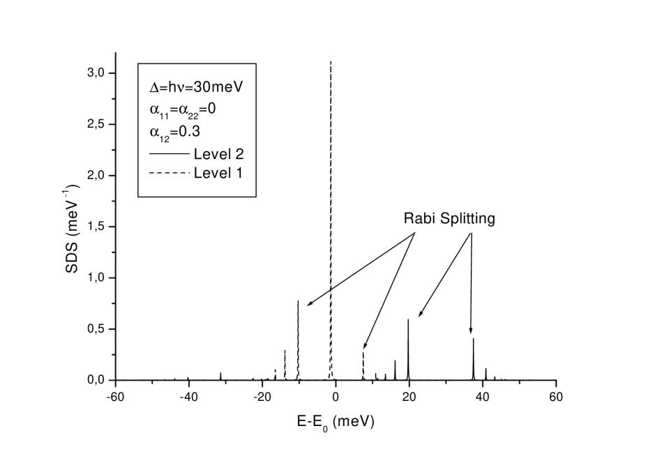
Figure 1: Calculated partial spectral densities of states corresponding to two electronic levels separated by $\Delta=30meV$ interacting with one optical phonon mode with $\hbar\omega_{0}=30meV$ (that is, $\Delta^{\prime}=0$). Only non-diagonal coupling was included ($\alpha_{12}=0.3$). Note the Rabi splitting in the polaron states and their shift to the lower energies.

The maximum number of phonons necessary to reproduce correctly several lowest-energy eigenvalues (which are of importance for relevant temperatures) depends on the coupling strengths but is not large. Taking just 10 as the maximum number of phonons allowed in the system, we obtained the eigenvalues coinciding with the analytical results of Ref.Mahan (for $\alpha_{12}=0$ , $\alpha_{11}=\alpha_{22}=0.2-0.3$) and formula (3) (for $\alpha_{12}=0.2-0.3$ , $\alpha_{11}=\alpha_{22}=0$ and using the RW approximation) to within $10^{-3}$meV. As an example, the SDS spectra calculated for the latter case (but beyond the RW approximation), are shown in Fig.1.

III Emission and absorption spectra

One can calculate the optical absorption and emission spectra by using the Kubo formula for the frequency-dependent dielectric functionMahan . The imaginary part of the dielectric function, which describes the absorption and emission properties, is related to the real part of the frequency–dependent conductivity by the relation

$$\mbox{Im }\epsilon(\omega)=\frac{4\pi}{\omega}\mbox{Re }\sigma(\omega).$$ (7)

According to the Kubo formula,

$$\mbox{Re }\sigma(\omega)=\frac{e^{2}}{m_{0}V}\frac{1}{2\omega}\int\limits_{-\infty}^{\infty}{dte^{i\omega t}\langle j^{+}(t)j(0)\rangle}.$$ (8)

We are interested in describing the transitions from an electron state (labelled $0$) in the valence band (which we assume is not coupled to phonons) to the states ($i=1,2$) in the conduction band, and vice-versa. Thus, the current operator is defined as

$$j=\sum\limits_{i=1}^{2}{p_{0i}\left(a_{i}^{+}a_{0}-a_{0}^{+}a_{i}\right)}.$$ (9)

The current-current correlation function is

$$\langle j^{+}(t)j(0)\rangle=\sum\limits_{i,i^{\prime}=1,2}{p_{0i}^{*}p_{0{i^{\prime}}}\left\langle\left[a_{0}^{+}(t)a_{i}(t)-a_{i}^{+}(t)a_{0}(t)\right]\left[a_{0}^{+}a_{i^{\prime}}-a_{i^{\prime}}^{+}a_{0}\right]\right\rangle}.$$ (10)

This expression can be developed into four expectation values. However, there are only two terms which contribute to the sum in Eq.(10). This occurs because $a_{i}|k\rangle$ vanishes if $|k\rangle$, an eigenstate of the Hamiltonian (1), is a state with zero electrons. The non-zero terms are

$$\langle a_{0}^{+}(t)a_{i}(t)a_{i^{\prime}}^{+}a_{0}\rangle=\frac{1}{Z}\sum\limits_{k}e^{-\beta E_{k}}e^{iE_{k}t}\left\langle k\left|a_{0}^{+}a_{i}e^{-iHt}a_{i^{\prime}}^{+}a_{0}\right|k\right\rangle$$

and

$$\langle a_{i}^{+}(t)a_{0}(t)a_{0}^{+}a_{i^{\prime}}\rangle=\frac{1}{Z}\sum\limits_{k}e^{-\beta E_{k}}e^{iE_{k}t}\left\langle k\left|a_{i}^{+}a_{0}e^{-iHt}a_{0}^{+}a_{i^{\prime}}\right|k\right\rangle$$

where $a_{i}\equiv a_{i}(0)$. These terms can be evaluated using the identity $1=\sum\limits_{k^{\prime}}|k^{\prime}\rangle\langle k^{\prime}|$ by inserting the unity between the $a$ operators. The result is:

$$\langle j^{+}(t)j(0)\rangle=\frac{1}{Z}\sum\limits_{k,\{m_{\nu}\}}\sum\limits_{i,{i^{\prime}}}p_{0i}^{*}p_{0{i^{\prime}}}e^{-\beta E_{k}}e^{i(E_{k}-E_{0})t}$$

$$\times\Bigl{[}{C_{i^{\prime}}^{k}}^{*}(\{m_{\nu}\})C_{i}^{k}(\{m_{\nu}\})-{C_{i}^{k}}^{*}(\{m_{\nu}\})C_{i^{\prime}}^{k}(\{m_{\nu}\})\Bigl{]}.$$ (11)

Using (11), performing the Fourier transformation in (8) and substituting in Eq.(7), we get the following expression for the imaginary part of the dielectric function:

$$\mbox{Im }\epsilon(\omega)=\left(\frac{2\pi e}{m_{0}\omega}\right)^{2}\frac{1}{VZ^{\prime}}\sum\limits_{i,{i^{\prime}}=1,2}\Bigl{\{}p_{0i}^{*}p_{0{i^{\prime}}}\sum\limits_{k,\{m_{\nu}\}}e^{-\beta\sum_{\nu}m_{\nu}\hbar\omega_{\nu}}{C_{i}^{k}}^{*}(\{m_{\nu}\})C_{i^{\prime}}^{k}(\{m_{\nu}\})$$

$$\times\Bigl{[}\delta\Bigl{(}\omega-(E_{k}-\sum_{\nu}m_{\nu}\hbar\omega_{\nu})\Bigl{)}+e^{-\beta(E_{k}-\sum_{\nu}m_{\nu}\hbar\omega_{\nu})}\delta\Bigl{(}\omega+(E_{k}-\sum_{\nu}m_{\nu}\hbar\omega_{\nu})\Bigl{)}\Bigl{]}\Bigl{\}}$$ (12)

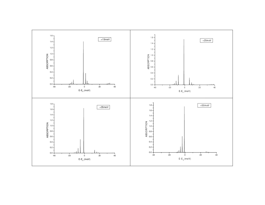
Figure 2: Calculated absorption spectra for different values of level spacing as indicated. All the other parameters are the same as for Fig.1.

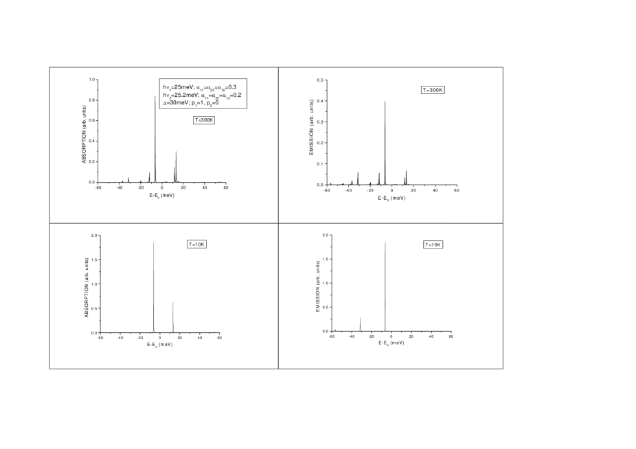
Figure 3: Absorption (left) and emission (right) spectra for a system of two exciton levels separated by $\Delta=30meV$ calculated for different temperatures. The excitons interact with two optical phonon modes of the energies $\hbar\omega_{1}=25meV$ and $\hbar\omega_{2}=25.2meV$. The electron-phonon coupling constants are indicated on the figure. The origin of the energy axis is chosen at the energy of the lowest exciton state ($E_{0}$).

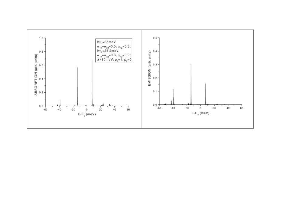
Figure 4: Absorption (left) and emission (right) spectra calculated for different (compared to Fig.3) values of the diagonal coupling constants.

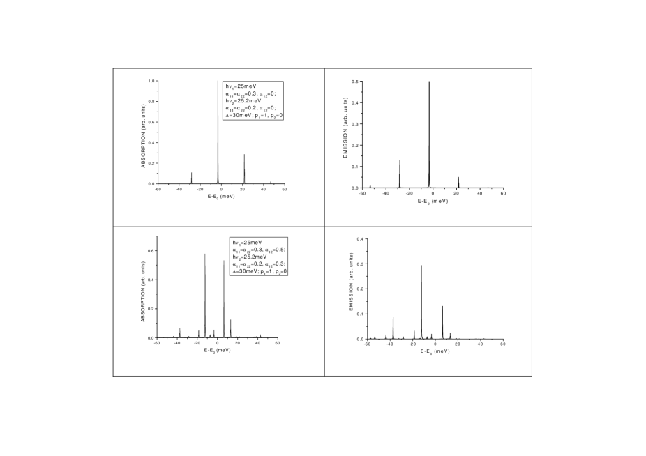
Figure 5: Absorption (left) and emission (right) spectra calculated for different values of the non-diagonal coupling constant (see the explanation to Fig.3).

where $Z^{\prime}=\sum\limits_{\{m_{\nu}\}}\exp{\Bigl{[}-\beta\sum_{\nu}m_{\nu}\hbar\omega_{\nu}\Bigl{]}}$. The terms in the second line of Eq.(12) correspond to the absorption and emission, respectively, of a photon of frequency $\omega$. Some absorption and emission spectra calculated for a hypothetical QD are presented in Figs.2-5 (the parameters are indicated on the figures), that demonstrate the effects of the diagonal and off-diagonal coupling strength, inter-level spacing and temperature on the optical properties of the dot. In these examples, we considered the lower exciton level optically active and the upper one inactive ($p_{2}=0$). Such a situation occurs in spherical II-VI (e.g. CdSe) QDs ($1s_{e}1S_{3/2}$ and $1s_{e}1P_{3/2}$ states, respectively)Efros .

IV Interaction with acoustic phonons

Interaction with confined longitudinal acoustic phonons, although mediated by a different (namely, deformation potential instead of Fröhlich) mechanism, can be considered in the same way as that with optical phonons and should result in series of closely spaced by still isolated spectral peaks. However, for any kind of QDs embedded in a certain matrix, there must be a spectral region where acoustic phonons are essentially delocalized and their energy varies in a continuous way. If the velocities of sound for the QD and matrix material are not very different, the density of acoustic phonon states should be similar to that of bulk crystals and these states can be characterized by a wavevector $\bf q$. This is the case of self-assembled QDsCazayous2000 and can be a reasonable approximation for a certain fraction of acoustic phonons in a spherical QD embedded in a dielectric matrix. In this section, we shall consider the interaction of an electron localized in the dot with acoustic phonons which are completely delocalized (see Appendix for details). The interaction, which occurs only inside the QD, is weak for each phonon mode (since it contains a factor $V_{QD}/V$, $V$ is the volume of the whole system). However, since the number of modes is virtually infinite, perturbation theory may fail. We shall avoid it. For this, we will have to neglect coupling between different electronic levels through acoustic phonons and consider a single electronic level coupled to arbitrary number of phonon modes. This approximation corresponds to the independent boson model Mahan , which is normally considered for optical phonons (see Sec. III). RecentlyKrummheuer ; Zimmermann2 , it was applied to acoustic phonons in a QD. Based on the exact solution of this model, we shall propose a different procedure which will lead us directly to the self-energy function of the electron or exciton. Later, this self-energy will be re-interpreted for the optical-phonon polaron.

The Hamiltonian of a system consisting of one electronic level and a continuum of acoustic phonon modes is:

$$H_{2}=a^{+}a\Bigl{(}\varepsilon_{0}+\sum\limits_{\bf q}{g_{\bf q}(b_{\bf q}^{+}+b_{\bf q})}\Bigl{)}+\sum_{\bf q}\hbar\omega_{\bf q}b_{\bf q}^{+}b_{\bf q}.$$ (13)

It can be diagonalized by the transformation to new bosonic operatorsMahan

$$B_{\bf q}=b_{\bf q}+\alpha_{\bf q}a^{+}a$$ (14)

where $\alpha_{\bf q}=({g_{\bf q}}/{\hbar\omega_{\bf q}})$. The energy spectrum is given by

$$E(\{N_{\bf q}\})=\varepsilon_{0}^{\prime}+\sum_{\bf q}\hbar\omega_{\bf q}N_{\bf q}$$ (15)

with $\varepsilon_{0}^{\prime}=\varepsilon_{0}-\sum_{\bf q}\alpha_{\bf q}^{2}\hbar\omega_{\bf q}$. Eigenstates of the Hamiltonian (13) can be expressed in terms of the pure phonon states,

$$|N_{\bf q}\rangle^{\prime}=\sum_{m_{\bf q}}C_{N}^{m}|m_{\bf q}\rangle.$$ (16)

Acting with the operator $B_{\bf q}^{+}B_{\bf q}$ on the wavefunction (16) we can find recurrent relations for the coefficients $C_{N}^{m}$:

$$N=(m+\alpha_{\bf q}^{2})(C_{N}^{m})^{2}+\alpha_{\bf q}\Bigl{[}\sqrt{m+1}C_{N}^{m+1}C_{N}^{m}+\sqrt{m}C_{N}^{m-1}C_{N}^{m}\Bigl{]}.$$ (17)

In linear (in the interaction with a single phonon mode $\bf q$) approximation, we get from (16) and (17):

$$|N_{\bf q}\rangle^{\prime}=p_{N_{\bf q}}\Bigl{[}\sqrt{N_{\bf q}}\alpha_{\bf q}|N_{\bf q}-1\rangle+|N_{\bf q}\rangle+\sqrt{N_{\bf q}+1}\alpha_{\bf q}|N_{\bf q}+1\rangle\Bigl{]}$$ (18)

where

$$p_{N_{\bf q}}=\frac{1}{\sqrt{1+(2N_{\bf q}+1)\alpha_{\bf q}^{2}}}.$$

The one-electron Green’s function corresponding to the Hamiltonian (13) can now be calculated using Eq.(4),

$$G(E)=\Bigl{\langle}\sum\limits_{\{m_{\bf q}\}}\frac{\prod\limits_{\bf q}\{\delta_{m_{\bf q},N_{\bf q}}+\alpha_{\bf q}^{2}[N_{\bf q}\delta_{m_{\bf q},N_{\bf q}-1}+(N_{\bf q}+1)\delta_{m_{\bf q},N_{\bf q}+1}]\}}{E-\varepsilon_{0}^{\prime}-\sum\limits_{\bf q}{\hbar\omega_{\bf q}(N_{\bf q}-m_{\bf q})}-i\eta}$$

$$\times\exp{\Bigl{[}-\sum\limits_{\bf q}{(2N_{\bf q}+1)\alpha_{\bf q}^{2}}\Bigl{]}}\Bigl{\rangle}$$ (19)

where the angular brackets stand for thermodynamical average and the exponential factor appeared from the product $\prod\limits_{\bf q}p_{N_{\bf q}}$. Taking into account only one-phonon processes, the thermodynamical average approximately replaces $N_{\bf q}$-s with the corresponding Bose factors $\bar{N}_{\bf q}=\Bigl{(}\exp{(\beta\hbar\omega_{\bf q})}-1\Bigl{)}^{-1}$ and the Green’s function can be written as:

$$G(E)=\Bigl{\{}\frac{1}{E-\varepsilon_{0}^{\prime}-i\eta}+\sum\limits_{\bf q}\Bigl{[}\frac{\alpha_{\bf q}^{2}\bar{N}_{\bf q}}{E-\varepsilon_{0}^{\prime}-\hbar\omega_{\bf q}-i\eta}+\frac{\alpha_{\bf q}^{2}(\bar{N}_{\bf q}+1)}{E-\varepsilon_{0}^{\prime}+\hbar\omega_{\bf q}-i\eta}\Bigl{]}\Bigl{\}}$$

$$\times{\Bigl{[}1+\sum\limits_{\bf q}{(2\bar{N}_{\bf q}+1)\alpha_{\bf q}^{2}}\Bigl{]}}^{-1}.$$ (20)

However, this equation (20) can be used only for quite a weak interaction or at very low temperatures. Although the interaction is weak for each phonon mode (all $\alpha_{\bf q}$ are small), the number of modes is large and the effective electron-phonon interaction is strong. A typical number of phonons interacting with the electron can be estimated as $Q=(2\bar{N}_{\bf q}+1)\alpha_{\bf q}^{2}$ and, for the model presented in Appendix, $Q>>1$ for temperatures usually used in the experiments. In these conditions, it is necessary to use the general equation (19).

The evaluation of the Green’s function from Eq.(19) can be made using a Monte-Carlo procedure. Instead of summing over all $3^{\mbox{N}}$ configurations $\{m_{\bf q}\}$ (N is the number of acoustic phonon modes), one can generate some $N_{MC}$ most probable configurations with $m_{\bf q}=(N_{\bf q}-1)$, $N_{\bf q}$, $(N_{\bf q}+1)$, occurring with the probabilities $\alpha_{\bf q}^{2}\bar{N}_{\bf q}p_{\bar{N}_{\bf q}}^{2}$, $p_{\bar{N}_{\bf q}}^{2}$, and $\alpha_{\bf q}^{2}(\bar{N}_{\bf q}+1)p_{\bar{N}_{\bf q}}^{2}$, respectively. Averaging over a sufficiently large $N_{MC}$ of such configurations, $G(E)$ is obtained including all the many-phonon processes.

Let us define the electron self-energy taking into account the interaction with acoustic phonons,

$$\Sigma(E)=E-G^{-1}(E).$$ (21)

In the one-phonon approximation, the explicit expression for the self-energy is:

$$\Sigma(E)=\varepsilon_{0}^{\prime}-(E-\varepsilon_{0}^{\prime})\sum\limits_{\bf q}{\alpha_{\bf q}^{2}(2\bar{N}_{\bf q}+1)}$$

$$+(E-\varepsilon_{0}^{\prime})^{2}\sum\limits_{\bf q}\Bigl{[}\frac{\alpha_{\bf q}^{2}\bar{N}_{\bf q}}{E-\varepsilon_{0}^{\prime}-\hbar\omega_{\bf q}-i\eta}+\frac{\alpha_{\bf q}^{2}(\bar{N}_{\bf q}+1)}{E-\varepsilon_{0}^{\prime}+\hbar\omega_{\bf q}-i\eta}\Bigl{]}.$$ (22)

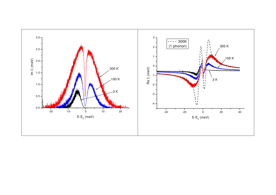
Figure 6: Imaginary (left) and real (right) parts of the self–energy for a single electronic level interacting with acoustic phonons, calculated for different temperatures using the Monte-Carlo technique explained in the text. The dashed curve was plotted using the one-electron approximation (Eq.(22)). The coupling constants were calculated as explained in the Appendix. The necessary material parameters were taken as follows: $\rho_{0}=5.8g/cm^{3}$, $c_{l}=3.8km/s$ and $a_{c}=3.5eV$. The QD radius $R$=2nm.

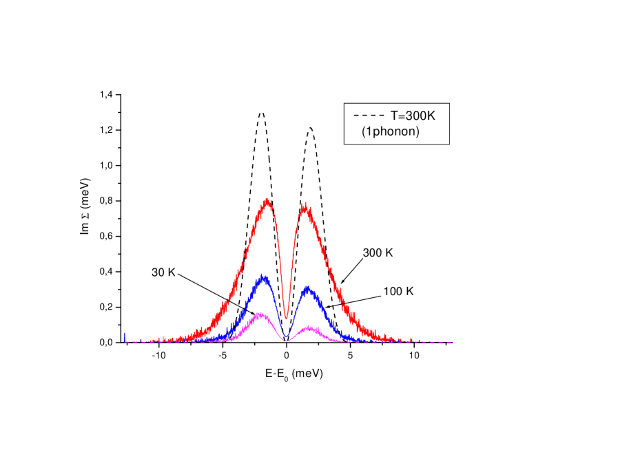
Figure 7: Imaginary part of the self–energy calculated for a $R$=4nm QD as explained for Fig.6. The dashed curve was plotted using one-electron approximation (Eq.(22)).

The spectral dependence of the self-energy corresponding to the Green’s function (Eq.(20)) obtained using the Monte Carlo procedure is presented in Figs.6,7. For comparison, we also calculated the self-energy using Eq.(22). The interaction constants $\alpha_{\bf q}$ derived in the Appendix were used in these calculations and the material parameters were taken as for CdSe, except for the deformation potential constant $a_{c}$, which was taken about 2 times smaller than the bulk value of the relative volume deformation potential between the valence and conduction bands Yu-Cardona . Such a choice is justified by the fact that only a fraction of acoustic phonons can be described by a propagating wave assumed in the Appendix.

Assuming that the broadening of the electronic levels produced by the interaction with acoustic phonons is small compared to the electronic level spacing, it is possible to include this interaction in our scheme of consideration of polaronic states proposed in the previous sections. Let us consider now the full Hamiltonian, which includes the interactions with both optical and acoustic phonons,

$$H_{3}=\sum\limits_{i=1}^{2}{\Bigl{(}\varepsilon_{i}+\sum\limits_{\bf q}{g_{\bf q}^{(i)}(b_{\bf q}^{+}+b_{\bf q})}\Bigl{)}a_{i}^{+}a_{i}}+\sum\limits_{ij}^{2}{\sum\limits_{\nu=1}^{N}{g_{ij}^{\scriptstyle\hfill\atop\scriptstyle\nu\hfill}}a_{i}^{+}a_{j}\left({b_{\nu}^{+}+b_{\nu}}\right)}$$

$$+\sum_{\bf q}\hbar\omega_{\bf q}b_{\bf q}^{+}b_{\bf q}+\sum\limits_{\nu=1}^{N}{\hbar\omega_{\nu}}{b_{\nu}^{+}b_{\nu}}$$ (23)

where $\alpha_{\bf q}^{(i)}$ denotes the acoustic phonon coupling constant for electronic level $i$. The Hamiltonian (23) can be rewritten in terms of the polaron states $|k\rangle$ by introducing the corresponding (fermionic) annihilation and creation operators $A_{k}^{+},A_{k}$. The electron-LO-phonon Hamiltonian (1) is then reduced to

$$H_{1}=\sum_{k}E_{k}A_{k}^{+}A_{k}$$

Using the expansion of the bare electronic states in terms of the polaron ones,

$$\left|i\right\rangle=\sum_{k}\sum_{\{m_{\nu}\}}\Bigl{(}C_{i}^{k}\left({\{m_{\nu}\}}\right)\Bigl{)}^{*}\left|k\right\rangle,$$

the term in (23) representing the interaction with acoustic phonons can be written as

$$\sum\limits_{i=1,2}\sum\limits_{\bf q}{g_{\bf q}^{(i)}(b_{\bf q}^{+}+b_{\bf q})}\sum_{k,k^{\prime}}\sum_{\{m_{\nu}\}}\Bigl{(}C_{i}^{k}\left({\{m_{\nu}\}}\right)\Bigl{)}^{*}C_{i}^{k^{\prime}}\left({\{m_{\nu}\}}\right)A_{k}^{+}A_{k^{\prime}}$$

$$=\sum\limits_{\bf q}{g_{\bf q}(b_{\bf q}^{+}+b_{\bf q})}\sum_{k}A_{k}^{+}A_{k}+\sum\limits_{\bf q}{\Delta g_{\bf q}(b_{\bf q}^{+}+b_{\bf q})}\sum_{k,k^{\prime}}t_{k,k^{\prime}}A_{k}^{+}A_{k^{\prime}}$$ (24)

where $g_{\bf q}=(g_{\bf q}^{(1)}+g_{\bf q}^{(2)})/2$, $\Delta g_{\bf q}=(g_{\bf q}^{(2)}-g_{\bf q}^{(1)})$, and

$$t_{k,k^{\prime}}=\sum_{\{m_{\nu}\}}\Bigl{\{}\left(C_{1}^{k}\left({\{m_{\nu}\}}\right)\right)^{*}C_{1}^{k^{\prime}}\left({\{m_{\nu}\}}\right)-\left(C_{2}^{k}\left({\{m_{\nu}\}}\right)\right)^{*}C_{2}^{k^{\prime}}\left({\{m_{\nu}\}}\right)\Bigl{\}}.$$

Neglecting the last term in (24), that is, assuming that the coupling to acoustic phonons is approximately the same for both electronic levels, we come to the Hamiltonian

$$H_{3}=\sum_{k}A_{k}^{+}A_{k}\Bigl{(}E_{k}+\sum\limits_{\bf q}{g_{\bf q}(b_{\bf q}^{+}+b_{\bf q})}\Bigl{)}+\sum_{\bf q}\hbar\omega_{\bf q}b_{\bf q}^{+}b_{\bf q}.$$ (25)

It can be diagonalized exactly in the same way as (13). The poles of the electron Green’s function (6) (as well as the absorption and emission peaks) are shifted according to the replacement $E_{k}\rightarrow E_{k}^{\prime}$,

$$E_{k}^{\prime}=E_{k}-\sum_{\bf q}\alpha_{\bf q}^{2}\hbar\omega_{\bf q}+\Bigl{\langle}\sum_{\bf q}\hbar\omega_{\bf q}(N_{\bf q}-m_{\bf q})\Bigl{\rangle},$$

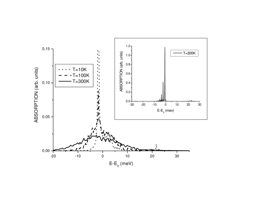
Figure 8: Absorption spectra calculated for an $R$=2nm CdSe QD including both optical and acoustic phonons for three different temperatures. Two optical phonon modes of the energies $\hbar\omega_{1}=25meV$ and $\hbar\omega_{2}=25.8meV$ and dimensionless interaction constants (divided by the corresponding phonon energies) $\alpha_{11}^{1}=-0.015$, $\alpha_{22}^{1}=0.027$, $\alpha_{12}^{1}=0.295$; $\alpha_{11}^{2}=0.063$, $\alpha_{22}^{2}=0.053$, $\alpha_{12}^{2}=0.095$ calculated in Ref.Vasilevskiy2 were used. The acoustic phonon parameters were taken as for Fig.6. The level spacing of $\Delta=80meV$ was assumed. The inset shows the $T=300$K spectrum without acoustic phonon contribution (at $T=10$K only the main peak is seen).

where, as before, $(N_{\bf q}-m_{\bf q})$ can be considered a random variable taking the values 1, 0 and -1 with the probabilities $\alpha_{\bf q}^{2}\bar{N}_{\bf q}p_{\bar{N}_{\bf q}}^{2}$, $p_{\bar{N}_{\bf q}}^{2}$, and $\alpha_{\bf q}^{2}(\bar{N}_{\bf q}+1)p_{\bar{N}_{\bf q}}^{2}$, respectively. The result is a similar broadening and a downward shift of all the polaron states contributing to the spectral density of states, absorption and emission, just like it happens in the one-level independent boson modelSR . It is equivalent to ascribing a spectral variable–dependent self-energy, $\Sigma(E-E_{p})$ (given by Eqs.(21) or (22)), to each pole of (6). As before, we can re-interpret this result for exciton–polaron, under the condition that we have no more than one exciton per QD. An example of spectra showing this effect is presented in Fig.8. The non-diagonal term with $t_{k,k^{\prime}}$ leads to acoustic phonon–mediated mixing of the polaron states. It will be considered in a future work.

V Discussion

Let us start the discussion by emphasizing that only in a hypothetical case when the phonon–mediated coupling of the lowest energy exciton state to all other states can be neglected (for example, in the limit of extremely strong confinement, such that $\Delta>>\hbar\omega_{0}$, or if $\alpha_{12}$ is small because of the symmetry of the corresponding wavefunctions), one can expect to observe Franck-Condon progressions in the emission and absorption spectra associated with this stateSR . This is the only case when the Huang-Rhys parameter describes the spectra in entirety. As it is obvious from Eq.(2), the diagonal coupling is proportional to the (integrated) difference between the electron and hole charge densities, which is non-zero mostly due to the fact that the conduction and valence bands in II-VI and III-V materials have different symmetry. Even if some further effects (like the presence of defects or strain, for example) contribute to the separation of the electron and hole clouds in spaceHeitz99 , one can hardly expect an order of magnitude increase of this parameter, compared to the calculated values cited in the Introduction. It means that the intensity of the LO phonon sidebands must be rather small and monotonically decreasing with the increase of the number of phonons.

However, in most cases the phonon–mediated interlevel coupling, at least between the subsequent exciton states, should be important. The off-diagonal interaction constant is likely to exceed the diagonal ones. For instance, if the two exciton levels are different by the hole state (e.g., $1s_{e}1S_{3/2}$ and $1s_{e}1P_{3/2}$ states in a spherical II-VI QD), it is easy to see from Eq.(2) that (neglecting the Coulomb interaction between the electron and hole),

$$g_{12}^{\nu}=e\int{\Psi_{1h}^{*}(\vec{r}_{h})\phi_{\nu}(\vec{r}_{h})\Psi_{2h}(\vec{r}_{h})d\vec{r}_{h}},$$ (26)

that is, there is no compensation effect for this interaction. The spectra calculated assuming only the off-diagonal interaction (Figs.1,2) show characteristic features known as Rabi splitting, which is obtained already in the RW approximation (see Eq.(3)) and has been observed experimentallyHameau . Contrary to the RW approximation, the exact results also show a downwards shift of the spectral lines (see Fig.1. In the RW approximation, the most intense peak should be situated exactly at $E-E_{0}=0$). Even if the upper level is dipole forbidden, its presence manifests itself by the spectral features seen in Fig.2. Note that the off-diagonal coupling is not resonant as one might expect thinking in terms of the Fermi’s Golden Rule. The manifold produced by the coupling persists even for quite a large detuning $\Delta^{\prime}>\hbar\omega_{0}$. Curiously, it is reminiscent of sidebands which might appear due to interaction with confined acoustic phonons.

When both diagonal and off-diagonal interactions are present, the effect is not just a sum of those owing to each of them, but also some additional spectral features appear (see Figs.3-5 showing the effect of different parameters). The stronger are the interactions, the richer the structure of the spectra. It should also be noted that the symmetry between the absorption and emission spectra, which is characteristic of the one-level independent boson model (see the upper panel of Fig.5), disappears when the off-diagonal interaction is included. This holds also at low temperatures where a small number of spectral features are seen (Fig.3, lower panel). Those below $E_{0}$ in the emission spectrum are due to the diagonal coupling to the lowest energy exciton state. The one seen in the absorption originates from the inter-level coupling.

Let us turn to the acoustic phonons. The explicit calculation leads to a self–energy which depends on the spectral variable in a sophisticated way. Accordingly, the line shape is quite different from the simple LorentzianKrummheuer ; Zimmermann2 . The noise seen in the calculated spectra of the self–energy (Figs.6,7) is due to the Monte Carlo procedure used when each configuration ${\{m_{\bf q}\}}$ of phonons produces a $\delta$-function and the number of Monte Carlo runs is finite ($N_{MC}=20000$ for Figs.6,7). The imaginary part of the self–energy vanishes at $\varepsilon_{0}^{\prime}$, so, the zero-phonon line (ZPL) at low temperatures remains a sharp $\delta$-like resonance situated between two asymmetric phonon sidebands, in accordance with experimentPalinginis ; Warming and previous theoretical studiesKrummheuer ; Zimmermann2 . Only for high temperatures the SDS generated by a single electronic level takes a bell-like shape similar to the Lorentzian. The calculated results also confirm the statement concerning the importance of the multiphonon processes which increase in smaller QDs (Fig.6). Turning to the exciton–polaron spectrum (Fig.8), the acoustic phonon–related broadening smears the discrete structure associated with optical phonons The multiplicity of the confined optical phonon modes also helps this. Below, we shall explain some previously published experimental findings, which were not clearly understood before, in terms of our calculated results.

“Strange” phonon replica

An experimental evidence of spectral features whose distance from ZPL is smaller than the LO phonon energy was found in several worksBissiri ; Ignatiev ; Fafard ; Odnolyub . Thinking in terms of the Franck-Condon progression, such peaks were attributed to additional (interface or disorder-activated acoustic) phonon modes, for some reason strongly coupled to the excitonOdnolyub . As it can be seen from Figs.3-5, in the presence of inter-level coupling, there are many spectral features that are not separated from ZPL (the most intense peak in all spectra) by (a multiple of) the optical phonon energy. Some of them persist at low temperatures. Such “strange” replica can be generated by a single phonon mode (long-wavelength LO phonon, neglecting its confinement) and their spectral positions are determined by the e-ph coupling constants. Thus, there is no need to invoke extra modes (for which it would be hard to justify their strong coupling to the exciton) in order to explain the discussed spectral features. The phonon–mediated inter-level coupling provides a simpler and more plausible explanation.

Anomalously strong 2LO phonon satellite

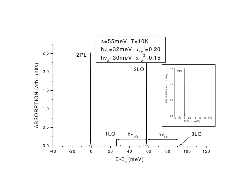
Figure 9: Low temperature absorption spectrum calculated for an InAs QD with the level spacing of $\Delta=55meV$ assuming two optical phonon modes (the energies are given on the figure) and neglecting coupling to acoustic phonons. The interaction constants used in this calculation are: $\alpha_{11}^{1}=0.005$, $\alpha_{22}^{1}=0.005$, $\alpha_{12}^{1}=0.2$; $\alpha_{11}^{2}=0.005$, $\alpha_{22}^{2}=0.005$, $\alpha_{12}^{2}=0.15$. Notice that three features above the zero-phonon line are separated by nearly the same energy, approximately equal to 31meV. The inset shows the corresponding emission spectrum.

As mentioned in the Introduction, several groups observed apparently phonon–related features in the absorption (but not in the emission) spectra of resonantly excited self–assembled QDsFafard ; Schmidt ; Lemaitre ; Toda ; Heitz . Given the relative weakness of the exciton-phonon interaction in such dots ($S<<1$), the most difficult to explain was the fact that the most intense satellite was not the 1LO phonon sideband but rather the 2LO or 3LO one. This effect was qualitatively understood as being due to a resonant coupling of the corresponding phonon replica of the ground state to the excited state of the excitonLemaitre . Considering a QD ensemble, one can think in terms of a multiphonon “filtering” of inhomogeneously distributed excited statesToda . However, when a single QD spectroscopy is usedLemaitre , such a resonance of the inter-level spacing with a multiple of the phonon energy is rather improbable. (Even though there are several confined optical phonon modes with slightly different energies, capable of considerable coupling to the exciton, this dispersion is only of the order of 1meV). The assumption of a reasonably strong off-diagonal coupling of the lowest and higher exciton states (not in a close resonance with a certain number of phonons) can account for anomalously strong $n$LO phonon sidebands. Fig.9 shows how peaks separated by energies approximately equal to that of the optical phonon can appear in the absorption spectra. We took a value of $\Delta$=55meV, typical of InAs/GaAs self-assembled QDs, and considered two optical phonon modes with the energies of 32 and 30 meV in order to simulate the experimental result of Lemaitre et alLemaitre . (The two modes can be interpreted as LO phonon in pure InAs and InAs-like LO phonon in the InGaAs alloy near the QD boundary, respectively). The values of $\alpha^{\nu}_{12}=0.2$ and 0.15 used in this calculation do not look extraordinarily high taking into account the argument presented above (see Eq.(26)) and the possible contribution of the optical deformation potential mechanism in this interaction. As it can be seen from Fig.9, the second strong absorption peak is not separated from ZPL by the energy $\Delta$ and can be called “2LO satellite”, since the weaker 1LO and 3LO ones also show up in the spectrum. The calculated spectrum is in a good agreement with the experimental observation of Ref.Lemaitre .

Homogeneous broadening of absorption lines

In structures of higher dimensionality, the temperature dependence of the homogeneous linewidth is described by the following relation,

$$\Gamma(T)-\Gamma(0)=\gamma_{ac}n_{ac}(T)+\gamma_{LO}n_{LO}(T)$$ (27)

where $\gamma_{ac}$ and $\gamma_{LO}$ are some constants and $n_{ac}$ and $n_{LO}$ the Bose factors for the acoustic and optical phonons, respectively. There is no reason for Eq.(27) be a good approximation for QDs, because it relies on the existence of a continuum of electronic states and also is limited to one-phonon scattering processes. Still it was used in HR1 ; Rakovich and some other publications to qualitatively describe the dependence $\Gamma(T))$ extracted from experimental absorption spectra of spherical QDs. It was found that this dependence, in the region from 77 to 300K, is much stronger than linear, similar to that predicted by the second term in Eq.(27), suggesting that there is some broadening related to the optical phonons. As it has been pointed out in the Introduction, interaction of localized electrons with optical phonons produces only additional discrete spectral lines. Consequently, the optical phonon related part of the broadening should not be understood literally, strictly speaking, the broadening occurs only because of the continuum of acoustic phonons. Our calculated Fig.8, where the interaction constants were taken as for a typical spherical CdSe QD studied in Ref.Rakovich , demonstrates this effect. The interaction with several optical phonon modes results in a series of closely spaced discrete peaks (see inset in Fig.8)) which is camouflaged by the acoustic phonons. The effective homogeneous broadening of the spectral lines may apparently depend on the equilibrium number of acoustic and optical phonons. Nevertheless, Eq.(27) is too simple to describe this effect even qualitatively, as found in Ref.Bayer using single QD spectroscopy.

Owing to the apparent similarity with systems of higher dimensionality, some authors associate the broadening discussed above with the optical phonon–assisted carrier relaxation. However, as it has been pointed outInoshita ; Levetas , this is not a lifetime (or irreversible scattering) effect. Indeed, the polaron states considered here are stationary states. The phonon-assisted relaxation can probably occur through an anharmonic decay of the phonons participating in the formation of the polaronic states, as suggested in Refs.Levetas ; Li and calculated in Ref.Verzelen . Our consideration of the polaron spectrum in the presence of acoustic phonons shows, however, another possibility, namely, the acoustic phonon–mediated transitions between different polaron states owing to the non-diagonal term in (24). The next step should consist of analyzing the efficiency of this mechanism. It is worth noting at this point that, contrary to the opinion of the authors of Ref.Jasak , such acoustic phonon-mediated transitions in the polaron spectrum should not be subject to phonon bottleneck, because there are plenty of polaron states due to different optical phonon modes differently coupled to the exciton. Many of them (which not necessarily show up in the spectra corresponding to thermal equilibrium) are separated by small energies within the band of acoustic phonons efficiently interacting with the polaron.

Up-converted PL

The up-converted or anti-Stokes photoluminescence (ASPL) is the emission of photons with energies higher than the excitation energy ($E_{exc}$). This effect was observed for colloidal II-VI QDs and discussed in several recent publicationsPoles ; Rak ; Wang . Additional information can be found in Ref.Filan . The ASPL occurs when an ensemble of QDs is excited at the very edge of the absorption spectrum, below the normal (i.e. excited with high energy photons) PL band. The principal experimental facts concerning this effect are the following:

(i) The ASPL intensity increases linearly with the excitation power Rak , which can be rather low.

(ii) The blue (anti-Stokes) shift between the ASPL peak and $E_{exc}$ does not depend significantly upon the QD size if $E_{exc}$ is chosen proportionally to the absorption peak energy (which depends upon the size)Rak . However, the shift increases with temperature and can range approximately from 20 to 150meVFilan .

(iii) If $E_{exc}$ increases (approaching the absorption peak) the ASPL also moves continuously towards higher energiesRak . Its intensity increases, and finally the spectrum transforms into the normal PL bandFilan .

(iv) The ASPL intensity increases strongly with temperature.

Possible ASPL mechanisms were discussed in Refs.Poles ; Rak ; Wang , but no definite conclusion was made. According to (i), processes like two-photon absorption and (since the possibility of emergence of more than one exciton per QD is negligible) Auger excitation can be excluded in this case. Therefore, it was suggested that incident photons excite electrons to some intermediate sub-gap states from which they eventually proceed to the higher energy (luminescent) states through the thermal effect. Some obscure surface states (SS’s) for which, as admitted by the authors of Ref.Wang , there is no any direct evidence, were suggested as those responsible for the sub-gap absorptionRak ; Wang .

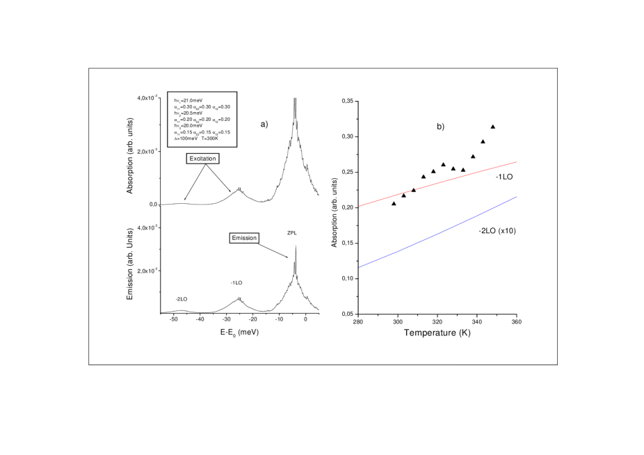
Figure 10: (a) Low-energy part of the absorption and emission spectra calculated for a hypothetical CdTe QD considering three optical phonon modes with parameters given on the figure. The acoustic phonon parameters were taken as for Fig.6. The level spacing $\Delta=100meV$, temperature 300K. (b) Temperature dependence of the integrated intensity of two sub-gap bands in the absorption spectrum (a) (lines) and experimental data of Ref.Rak (points) showing the temperature dependence of the ASPL peak amplitude.

From our point of view, the participation of sub-gap SS’s (even if they exist in the passivated colloidal QDs) is unlikely in virtue of the experimental results (ii) and (iii). In fact, it would require the SS’s energy have approximately the same dependence on the QD size as that of the confined electronic states in the dots, in obvious contradiction with what should be expected from the general point of view. At the same time, there exist naturally formed sub-gap states, which are separated from the fundamental absorption line (i.e., ZPL) by energies which are only weakly dependent on the QD size. These are the red-shifted optical phonon replica. Fig.10a presents the lower–energy side of a calculated QD absorption spectrum showing two sub-gap bands (designated as “-1LO” and “-2LO”) through which the dot can be excited. The excited QD then will emit a photon most likely having the ZPL energy. The probability of such an up-conversion process increases with temperature because so does the integrated intensity of “-1LO” and “-2LO” absorption bands (shown calculated in Fig.10b). The experimental temperature dependence of the ASPL intensity measured in Ref.Rak can be understood taking into account that, at a certain temperature, further red–shifted satellites (whose intensity depends more strongly on the temperature) become more efficient. The situation is complicated by the distribution of the QD size, so that $E_{exc}$ can match different “$-n$LO” bands of dots of several different sizes. This agrees qualitatively with the experimentally observed increase in the anti-Stokes shift with temperatureFilan . Modeling of the ensemble effects involved in the ASPL phenomenon is beyond the scope of this paper and will be considered in a future work. Nevertheless, we believe that our model explains, at least qualitatively, the principal experimental facts concerning the ASPL.

In conclusion, we proposed a non-perturbative approach for the calculation of the polaronic effects in QDs, which allows the consideration of electronic levels coupled through the interaction with several confined phonon modes. Using this approach, we were able to show that the polaronic effects are significant even when the interlevel spacing is quite away from resonance with the optical phonon energies. We demonstrated that this opens the possibility to account for some previously published and not clearly understood experimental data. We also presented an explicit calculation of the spectral line shapes because of the diagonal interaction of acoustic phonons with the original electronic levels and suggest that the same interaction may be responsible for relaxation of the polaron entity to lower energies.

VI Acknowledgments

This work was supported by the FCT (Portugal) through project FCT-POCTI/FIS/10128/98, ICCTI-CNPq (Portugal-Brazil) Cooperation Program and Brazilian agencies CNPq and FAPERJ. The authors are grateful to S.Filonovich for discussions of the ASPL and to T.Warming for providing the manuscript of Ref.Warming prior to publication.

*

Appendix A Electron-acoustic-phonon coupling rates

The following simple model was used to estimate the rates $\alpha_{\bf q}$ of electron coupling to longitudinal acoustic phonons. Assuming that LA phonons are completely delocalized, that is, neglecting acoustic impedance at the interface between the QD and matrix, the displacement can be written as

$$u_{z}=\Bigl{(}\frac{\hbar}{2\omega_{q}\rho_{0}V}\Bigl{)}^{1/2}\mbox{Re }e^{i(qz-\omega_{q}t)},$$

where $\rho_{0}$ is the density. For the deformation potential interaction mechanism, the dimensionless coupling constant is Yu-Cardona

$$\alpha_{\bf q}=\frac{a_{c}}{\hbar\omega_{\bf q}}\int|\psi|^{2}\mbox{div}{\bf u}({\bf q})dV,$$

where $a_{c}$ is the bulk deformation potential and $\psi$ the electron wavefunction. Considering the lowest conduction band state in a spherical QD of radius $R$, with infinite barriers, the wavefunction is Efros :

$$\psi=\sqrt{\frac{1}{2\pi R}}\frac{\sin{(\pi r/R)}}{R}\qquad(r\leq R).$$

Using these expressions, we obtain

$$\alpha_{\bf q}=a_{c}\Bigl{(}\frac{1}{2\hbar\omega_{q}\rho_{0}Vc_{l}^{2}}\Bigl{)}^{1/2}I(qR)$$ (28)

where $c_{l}$ is the longitudinal sound velocity,

$$I(y)=2\pi^{2}\int_{0}^{1}j_{0}(y\cdot x)j_{0}^{2}(\pi x)x^{2}dx$$ (29)

and $j_{0}$ is the spherical Bessel function. The integral in (29) can be expressed in terms of the integral sinus as

$$\frac{1}{2}\{\mbox{Si}(y)-\frac{1}{2}[\mbox{Si}(y+2\pi)+\mbox{Si}(|y-2\pi|)]\}.$$

The function $I(y)$ decreases from 1 for $y=0$ to nearly zero for $y\geq 5$.

Figures

References

- (1) L. Bányai and S.W. Koch, Semiconductor Quantum Dots (World Scientific, Singapore, 1993).
- (2) R. Heitz, in Nano-Optoelectronics. Concepts, Physics and Devices, edited by M. Grundmann (Springer-Verlag, Berlin, 2002), p.239.
- (3) T.D. Krauss, F.W. Wise and D.B. Tanner, Phys. Rev. Lett. 76, 1376 (1996).
- (4) M.P. Chamberlain, C. Trallero-Giner and M. Cardona, Phys. Rev. B 51, 1680 (1995).
- (5) M.I. Vasilevskiy, A.G. Rolo, M.V. Artemyev, S.A. Filonovich, M.J.M. Gomes and Yu.P. Rakovich, Phys. Stat. Sol. (b) 224, 599 (2001).
- (6) M.I. Vasilevskiy, A.G. Rolo, M.J.M. Gomes, O.V. Vikhrova and C. Ricolleau, J. Phys.: Condensed Matter 13, 3491 (2001).
- (7) E.P. Pokatilov, S.N. Klimin, V.M. Fomin, J.T. Devreese and F.W. Wise, Phys. Rev. B 65, 075316 (2002).
- (8) P. Verma, W. Cordts, G. Irmer and J. Monecke, Phys. Rev. B 60, 5778 (1999).
- (9) L. Savoit, B. Champagnon, E. Duval, I.A. Kudriavtsev and A.I. Ekimov, J. Non-Cryst. Solids 197, 238 (1996).
- (10) D.A. Tenne, V.A. Haisler, A.I.Toropov, A.K. Bakarov, A.K. Gutakovsky, D.R.T. Zahn and A.P. Shebanin, Phys. Rev. B 61, 13785 (2000).
- (11) J.R. Huntzinger, J. Groenen, M. Cazayous, A. Mlayah, N. Bertru, C. Paranthoen, O. Dehaese, H.Carrére, E. Bedel and G. Armelles, Phys. Rev. B 61, 10547 (2000).
- (12) P. Palinginis, S. Tavenner, M. Lonergan and H. Way, Phys. Rev. B 67, 201307 (2003).
- (13) T. Warming, F. Gufferth, R. Heitz, C. Kaptein, P. Brunkov, V. M. Ustinov and D. Bimberg, Semicond. Sci. Technol. (to be published).
- (14) B. Krummheuer, V.M. Axt and T. Kuhn, Phys. Rev. B 65, 195313 (2002).
- (15) S. Nomura and T. Kobayashi, Phys. Rev. B 45, 1305 (1992).
- (16) Y. Cheng, S. Huang, J. Yu anf Y. Chen, J. Lumin. 60-61, 786 (1994).
- (17) R. Heitz, I. Mukhametzhanov, O. Stier, A. Madhukar and D. Bimberg, Phys. Rev. Lett. 83, 4654 (1999).
- (18) M.G. Bawendi, P.J. Carroll, W.L. Wilson and L.E. Brus, J. Chem. Phys. 96, 946 (1992).
- (19) V. Jungnickel anf F. Henneberger, J. Lumin. 70, 238 (1996).
- (20) M. Bissiri, G. B. von Högersthal, A.S. Bhatti, M. Capizzi, A. Frova, P. Frigeri and S. Franchi, Phys. Rev. B 62, 4642 (2000).
- (21) I.V. Ignatiev, I.R. Kozin, V.G. Davydov, S.V. Nair, J.-S. Lee, H.-W. Ren, S. Sugou and Y. Masumoto, Phys. Rev. B 63, 075316 (2001).
- (22) V.M. Fomin, V.N. Gladilin, J.T. Devreese, E.P. Pokatilov, S.N. Balaban and S.N. Klimin, Phys. Rev. B 57, 2415 (1998).
- (23) H. Rho, L.M. Robinson, L.M. Smith, H.E. Jackson, S. Lee, M. Dobrowolska and J.K. Furdyna, Appl. Phys. Lett. 77, 1813 (2000).
- (24) S. Fafard, R. Leon, D.Leonard, J.L. Merz and P.M. Petroff, Phys. Rev. B 52, 5752 (1995).
- (25) K.H. Schmidt, G. Medeiros-Ribeiro, M. Oestereich, P.M. Petroff and G.M. Döhler, Phys. Rev. B 54, 10435 (1996).
- (26) A. Lemaitre, A.D. Ashmore, J.J. Finley, D.J. Mowbray, M.S. Skolnick, M. Hopkinson and T.F. Krauss, Phys. Rev. B 63, 161309 (2001).
- (27) Y. Toda, O. Moriwaki, M. Nishioka and Y. Arakawa, Phys. Rev. Lett. 82, 4114 (1999).
- (28) R. Heitz, M. Veit, N.N. Ledentsov, A. Hoffmann, D. Bimberg, V.M. Ustinov, P.S. Kop’ev and Zh.I. Alferov, Phys. Rev. B 56, 10435 (1997).
- (29) Yu.P. Rakovich, M.I. Vasilevskiy, M.V. Artemiev, S.A. Filonovich, A.G. Rolo, D.J. Barber and M.J.M. Gomes, in Proc. 25-th Int. Conf. on the Physics of Semiconductors, edited by N. Miura and T. Ando (Berlin, Springer), part II, p.1203.
- (30) S. Marcinkevicius, A. Gaarder and R. Leon, Phys. Rev. B 64 115307 (2001).
- (31) S. Hameau, Y. Guldner, O. Verzelen, R. Ferreira, G. Bastard, J. Zeman, A. Lemaitre and J.M. Gérard, Phys. Rev. Lett. 83, 4152 (1999).
- (32) T. Inoshita and H. Sakaki, Phys. Rev. B 56, 4355 (1997).
- (33) K. Král and Z. Khás, Phys. Rev. B 57, 2061 (1998).
- (34) T. Stauber, R. Zimmermann and H. Castella, Phys. Rev. B 62, 7336 (2000).
- (35) L. Jasak, P. Machnikowski, J. Krasnyi and R. Zöller, Eur. Phys. J. D 22, 319 (2003).
- (36) S.A. Levetas, M.J. Godfrey and P. Dawson, in Proc. 25-th Int. Conf. on the Physics of Semiconductors, edited by N. Miura and T. Ando (Springer-Verlag, Berlin), part II, p.1333.
- (37) M.I. Vasilevskiy, E.V. Anda and S.S. Makler, in Proc. 26-th Int. Conf. on the Physics of Semiconductors, edited by A.R. Long and J.H. Davies, Institute of Physics Conference Series Number 171 (IOP Publ., Bristol, 2002), P229.
- (38) R. Zimmermann and R. Runge, in Proc. 26-th Int. Conf. on the Physics of Semiconductors, edited by A.R. Long and J.H. Davies, Institute of Physics Conference Series Number 171 (IOP Publ., Bristol, 2002), M3.1.
- (39) S. Schmitt-Rink, D.A.B. Miller and D.S. Chemla, Phys. Rev. B 35, 8113 (1987).
- (40) V. Savona, F. Bassani and S. Rodriguez, Phys. Rev. B 49, 2408 (1994).
- (41) G.D. Mahan, Many-Particle Physics (Kluwer Academic, New York, 2000).
- (42) P. Meystre and M. Surgent III, Elements of Quantum Optics (Springer-Verlag, Berlin, 1998), p.287.
- (43) J. Bonc̆a and S.A. Trugman, Phys. Rev. Lett. 75, 2566 (1995).
- (44) S.S. Makler, E.V. Anda, R.G. Barrera and H.M. Pastawski, Braz. J. Phys. 24, 330 (1994).
- (45) E.M. Lifshitz and L.P. Pitaevskii, Statistical Physics, Part II (Moscow, Nauka, 1978), p.173.
- (46) A.I. Ekimov, F. Hache, M.C. Schanne-Klein, D.Ricard, C.Flytzanis, I.A. Kudryavtsev, T.V. Yazeva, A.V. Rodina and Al.L. Efros, J. Opt. Soc. Am. B 10, 100 (1993).
- (47) P.Y. Yu and M. Cardona, Fundamentals of Semiconductors (Springer-Verlag, Berlin, 1996).
- (48) M.A. Odnoblyudov, I.N. Yassievich and K.A. Chao, Phys. Rev. Lett. 83, 4884 (1999).
- (49) M. Bayer and A. Forchel, Phys. Rev. B 65, 041308 (2002).
- (50) X.Q. Li, H. Nakayama and Y. Arakawa, Phys. Rev. B 59, 5069 (1999).
- (51) O. Verzelen, G. Bastard and R. Ferreira, Phys. Rev. B 66, 081308 (2002).
- (52) E. Poles, D.C. Selmarten, O.I. Mićić and A.J. Nozik, Appl. Phys. Lett. 75, 971 (1999).
- (53) Yu.P. Rakovich, S.A. Filonovich, M.J.M. Gomes, J.F. Donegan, D.V. Talapin, A.L. Rogach and A. Eychmüller, Phys. Stat. Sol. (b) 229, 449 (2002); Yu.P. Rakovich, A.A. Gladyshchuk, K.I. Rusakov, S.A. Filonovich, M.J.M. Gomes, D.V. Talapin, A.L. Rogach and A. Eychmüller, J. Appl. Spectrosc. 69, 444 (2002).
- (54) X. Wang, W.W. Yu, J. Zhang, J. Aldana, X. Peng and M. Xiao, Phys. Rev. B 68, 125318 (2003).
- (55) S.A. Filonovich, Optoelectronic Properties of Semiconductor Quantum Dot Ensembles , PhD Thesis, University of Minho, Braga, Portugal, 2003.