Notes on RVB-Vanilla by Anderson et al.

Abstract

The claims made for the Resonating Valence Bond ideas for the Cuprates in a recent paper by Anderson et al. on the basis of a variational calculation are discussed.

I Introduction

Within weeks of the confirmation of the discovery of high temperature superconductivity in the cuprates by Bednorz and Muller, Anderson[1] suggested an explanation of the phenomena and called it resonating valence bonds (RVB). Despite an enormous theoretical effort by the international scientific community, systematic or consistent theoretical results have been hard to obtain on this idea for the model proposed by Anderson for the cuprates. When some specific predictions were made based on the general ideas or approximate calculations, experiments did not conform.

In a curious recent note Anderson, Lee, Randeria, Rice, Trivedi and Zhang (ALRRTZ) [2]. put forth that the variational calculations that were done over a decade ago based on Anderson’s ideas and have been revived [3] recently, support the ideas of RVB for the cuprates. They also reiterate that the Hubbard /t-J model, also proposed by Anderson is a sufficient model for the essential physics of the cuprates.

In this note I point out the following:

(1) The principal result of the variational calculations discussed by ALRRTZ is contrary to a vast array of experimental results. This disagreement is of a fatal nature for ideas which the variational calculation is taken to support.

(2) The properties of the Hubbard/t-J model cannot be adequately studied using the wavefunctions with the limited variational degree of freedom employed by ALRRTZ.

(3) In view of (1) and several other experimental and theoretical results, the Hubbard/t-J model is itself inadequate as a model for the Cuprates.

II Experiments and the results from the chosen Wavefunction

The chosen variational wavefunction is the d-wave superconducting wavefunction with projection to remove double occupation:

$$\Phi=\bar{P}\phi_{BCS}\left(\Delta({\bf k})\right).$$ (1)

$\bar{P}$ is the projection operator and $\Delta({\bf k})$ is the the d-wave BCS order parameter function with a variational parameter of magnitude $\Delta_{0}$. The principal result of the calculations is that the ground-state energy is minimized when $\Delta_{0}$ varies with $x$, the deviation from half-filling as shown schematically in figure (1), while the superconducting long-range order parameter $|\Psi|$ has a dependence with $x$ as also sketched in the figure. $\Delta_{0}$ is interpreted to represent the magnitude of the experimentally observed pseudogap. A corollary to fig. (1) is a phase diagram sketched in fig. (2), where $T_{p}^{A}$ marks the crossover temperature to pseudogap properties. The validity of the argument can be tested by comparing the results of figs. (1) and (2) with experiment. Other comparisons with experiment are not meaningful if this test fails.

FIG. 1.: The calculated variation of the parameter $\Delta_{0}$ in the wavefunction Eq. (1) and the calculated magnitude of the superconducting order parameter with x; adapted from Ref. (2)

FIG. 2.: The Phase diagram in the $T-x$ plane implied by calculations reported in Ref. (2)

The authors acknowledge that the wavefunction does not correctly give the region near $x=0$, where the model studied as well as the Cuprates have an AFM ground state. An unasked question is : At what x does the chosen RVB variational wavefunction have a lower energy than a wavefunction describing AFM at appropriate wave-vectors ${\bf Q}(x)$? They also acknowledge that their approach is no help in understanding the universal normal state properties for compositions near those for the highest $T_{c}$. I will return to both these points; first, let us compare the claims made with the experiments.

A crucial feature of Fig. (1) is that the parameter $\Delta_{0}$ is finite throughout the superconducting region $x_{min}<x<x_{max}$. I summarize evidence below that, in experiments, the pseudogap properties disappear above a critical composition $x_{c}$ within the superconducting region. Moreover experiments show that a singularity exists at $x_{c}$, the Quantum Critical Point (QCP) in the limit $T\rightarrow 0$. If $T_{c}$ is reduced by application of a magnetic field, the normal state anomalies continue to lower temperatures. The pseudogap region as well as the Fermi-liquid region emanate from $x_{c}$. Any theory which is smooth across $x=x_{c}$ can then not be a theory for the Cuprates. The universal phase diagram of the cuprates [4] is as sketched in fig. (3).

The evidence is diverse and mutually consistent:

(1) Tunneling Measurements: The most direct is the measurement of pseduogap by tunneling by Alff et al. [5] in two electron doped superconductors by reducing $T_{c}$ on applying a magnetic field. The central observations are (a) for $x<x_{c}$ within the superconducting dome, the characteristic pseudogap feature in tunneling conductance is observed while the superconducting gap feature disappears as $T_{c}(H)$ is reduced to 0, (b) This feature appears at a temperature $T_{p}(x)$ below $T_{c}(x)$ at $H=0$, (c) the magnitude of the pseudogap for three different samples with $T_{p}(x)$ below $T_{c}$, and $T_{p}(x)$ itself, extrapolate to zero at an $x_{c}$ inside the superconducting dome.

(2) Resistivity near $T=0$: In the region above $T_{c}(x)$ and below a temperature characterized by $T_{p}(x)$, a change in the temperature dependence of the resistivity from linear to a higher power is observed. Similarly below a temperature $T_{F}(x)$ for $x>x_{c}$, a change in the power law tending towards the Fermi- liquid value of 2 is observed. This is observed in all the cuprates studied. Fig.(4) organizes the data in a number of compounds [8].

A linear temperature dependence of resistivity at low temperatures cannot occur without a putative singularity in the fluctuation spectra at $T=0$. Measurements in a large enough magnetic field to drive $T_{c}$ to 0 show that the linearity persists in an increasingley narrower region of $x$ as $T_{c}$ is decreased and persists at least down to $40mK$ in one cuprate compound [6] and down to at least 2 K in another [7]. To within the finest composition variation studied, $\delta x=0.01$, the resistivity power law changes to higher values on either side of $x_{c}$.

FIG. 3.: The universal Phase diagram for the Cuprates; from Ref.(4)

(3) Hall effect near $T=0$ [6]: In the case of one of the class of compounds whose $T_{c}$ is reduced to $0$ by a magnetic field, the Hall coefficient has been measured at low temperatures. It shows a singular derivative at $x\approx x_{c}$.

(4) Transport properties above $T_{c}(x)$: Actually, it is not necessary to study the properties near $T=0$ to rule out a pseudogap region beyond an $x_{c}$ in the superconducting range of $x$. If fig. (2) were true, the universal normal state anomalies would change to the pseudogap properties for any $x$ for temperatures below $T^{A}_{p}(x)$ and above $T_{c}(x)$. The data does not sustain this point of view. The resistivity data consistent with the phase diagram (3) has been shown in fig. (4). Wuydt et al.[9] have shown that the determination of $T_{p}(x)$ by thermodynamic measurements, specific heat and magnetic susceptibility as well as the Cu-nuclear relaxation rate is consistent with that from resistivity. Recent measurements of the optical conductivity [10] for various compositions are also consistent with the phase diagram (3).

In a very recent paper, Naqib et al.[11] have measured the resistivity of $Y_{1-x}Ca_{x}Ba_{2}(Cu{1-y}Zn_{y})_{3}O_{7-\delta}$ over a wide range of $x$ and $y$ and in a magnetic field. Just as a magnetic field, $Zn$ reduces $T_{c}$ without affecting the pseudogap. They can thereby observe the variation of $T_{p}$ below the un-Zn-doped and zero magnetic field $T_{c}$. $T_{p}$ continues below this $T_{c}$, extrapolating to a finite value well within the superconducting dome.

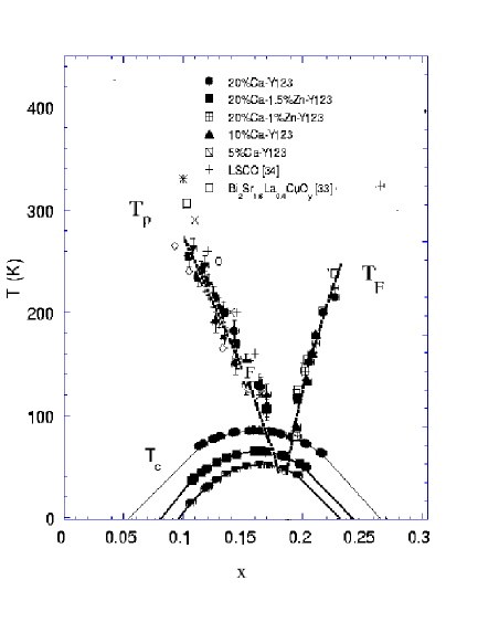
FIG. 4.: Organization of the Resistivity data for a number of Cuprates: In the region between the set of points indicated by $T_{c},T_{p},T_{F}$, the resistivity is linear in temperature. It has a different dependence in other regions. Figure taken from Ref.(8).

(5)Thermodynamic Measurements: ALRRTZ [2] quote only the thermodynamic measurements and analysis by Loram et al.[12] both in the normal state and for the superconducting condensation energy, and claim not to understand how the conclusions were reached. Actually the conclusions of Loram et al. are consistent with the existence of a QCP and all the experiments quoted above.This is discussed further below in connection with fig.(5).

(6) Raman Susceptibility: Careful measurements of Raman intensity in the compound 123 near $x=x_{opt}$, the composition for the highest $T_{c}$, show [13] that the susceptibility has the scale invariant form

$$Im~{}\chi(\omega/T)~{} \propto ~{}\omega/T,~{}~{}for~{}\omega/T~{}\ll~{}1$$ (2)

$$\propto ~{}~{}constant,~{}~{}for~{}\omega/T~{}~{}\gg~{}1.$$ (3)

More complete are measurements [14] in the compound 248. At stoichiometry, this compound displays the pseudogap properties with a characteristic change in resistivity from linear to that of the pseudogap behavior below $T_{p}\approx 200K$ and a $T_{c}$ of 80 K. Under pressure P, $T_{c}$ continuously rises to 110 K at a P of 100 kbar; simultaneously $T_{p}$ decreases and is invisible above a P about 80 kbar [15]. Raman measurements under pressure reveal the form of Eq. (2) near 100 kbar but at lower P one finds a characterstic infra-red cut-off proportional to $T_{p}(P)$.

In their paper ALRRTZ reproduce the magnitude of a gap deduced from the photoemission experiments [16] which indeed varies with $x$ in the manner similar to fig. (1). This gap is deduced at low temperatures from experiments in the superconducting phase. This may appear reasonable enough. After all the comparison is being made to a parameter in a ground state wavefunction. Actually, this is a specious argument if $\Delta_{0}$ is understood to represent the pseudogap. A tunneling measurement made below $T_{c}$ will show a gap which is zero only when both the pseudogap and the superconducting gap are zero because the gap measured is is an appropriate combination of the pseudogap $D(x)$ and the superconducting gap $\Delta_{sc}(x)$; for instance

$$gap=\sqrt{|D({\bf k})|^{2}+|\Delta_{sc}({\bf k})|^{2}}$$ (4)

To measure the pseudogap one must kill the superconducting gap as Alff et al. [5] have done, as discussed above. The total gap in zero field and at low temperatures then goes to zero only for $x>x_{max}$. Alternately one may deduce the pseudogap from measurements above $T_{c}$. Loram et al. have done this through modelling their thermodyanmic measurements. A comparison of their deduced values of the pseudogap as a function of $x$ with those obtained from tunneling and photoemission at low temperature is shown [17] in fig.(5). The two sets of gaps do follow a relation not inconsistent with Eq. (3) if $\Delta_{sc0}$ is proportional to $T_{c}(x)$.

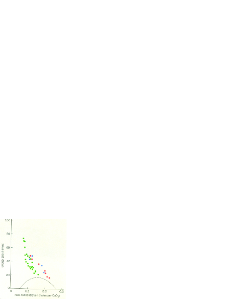
FIG. 5.: The energy gap in the normal state determined by fitting to the specific heat data with a model density of states by Loram et al. is shown in green. The tunneling experiments well below $T_{c}$ give the gap shown in red in agreement with ARPES shown in blue.

III Restricted Variational freedom

The variational results are at odds with the phase diagram for the cuprates. Are they a good representation of the physics of the t-J model? What does the variational parameter $\Delta_{0}$ really represent? In a model with strong local interactions $U>>t$, there must be a transfer of the distribution function $n({\bf k})$ from below the Fermi-vector to above compared to non-interacting electrons. In the wavefunction, Eq. (1), $\Delta_{0}$ is the only parameter to accomplish this physics. There is then simply no choice but for the calculations to exhibit a pseudogap. It is put in by hand without comparing the ground state energy with other wavefunctions which accomplish the same physics. The choice of Eq. (1) automatically ensures $\Delta_{0}\approx J$ for $x\approx 0$ with a decline to $\approx 0$ for large enough $x$. A Fermi-liquid, accomplishes the same physics with a discontinuity $z$ in $n({\bf k})$ at ${\bf k}_{F}$. $z$ changing smoothly from $0$ near $x=0$ to $1$ for large enough $x$. Much more relevant for the physics of the t-J model would be to compare the ground state energy using Eq. (1) with that for a wavefunction representing AFM order at a wave-vector ${\bf Q}(x)$, also projected to remove double-occupation. We know the wavefunction (1) is wrong for the t-J model near $x=0$ only because the experiments say the region near $x=0$ is AFM. How far does this problem with the wavefunction persist. Only comparison of the energy with an AFM wavefunction can tell. Based on the results of the mean-field calculations and several numerical calculations, my conjecture is that the regime of AFM for the t-J model is much more extended than in the experiments and that in variational calculations the phase diagram will show AFM followed by a co-existing region of AFM and d-wave superconductivity followed by d-wave superconductivity alone. The physics is much the same as that for d-wave superconductivity derived from AFM fluctuations with numerical corrections from Fermi-liquid effects [18].

This is not to say that the t-J model has a superconducting ground state above some $x$. As Anderson et al. point out, numerical evidence on this issue is divided. But, from the perspective of a theory of the cuprate phenomena this issue is incidental. Even if the ground state of the t-J model were to be superconducting, it cannot be a model for the Cuprates unless it can give a phase diagram similar to Fig. (3).

IV Model for Cuprates

It was suggested [19] that a unique property of the cuprates is that the ionization energy of the $Cu^{++}$ ions is very close to the affinity energy of $O^{--}$. (This is what makes the half-filled Cuprates charge transfer insulators[20]). Their difference $\epsilon_{pd}$ is similar to the kinetic energy parameter $t_{pd}$ and estimates of the screened nearest neighbor Cu-O ionic interactions V. In this condition, in the metallic phase charge fluctuations exist almost equally on Cu and O ions and that new physics can arise in a model with three dynamic degrees of freedom per unit cell (two Oxygens and one Copper)due to the ionic interactions. Anderson et al. argue instead that as observed in experiments there is only one band near the Fermi-surface and in any case the three orbital model may be reduced to a one effective orbital model by a canonical transformation. In this canonical transformation, they ignore the interactions represented by V. It is easy to show that for $zV\geq t_{pd},\epsilon_{p}-\epsilon_{d}$, where z is the number of nearest neighbors, this canonical transformation does not converge.

The argument has never been that there is more than one band near the chemical potential. The relevant question is what is the nature of the wavefunctions in this band and the effective interactions among one-particle excitations of the band after the states far from the chemical potential (in band calculations) are eliminated. That new physics arises in the general model (3-orbitals and ionic interactions as well as local interactions) [19] is known from two exact solutions : (a) A local model, which bears the same relation to the general model as the Anderson model for local moments bears to the Hubbard model. A QCP is found in the model with logarithmic singularities unlike the Ground state singlet of the Anderson or Kondo model [21]. (b) Long one -dimensional —-Cu-O-Cu-O— chains on which extensive numerical results [22] have been obtained. This model gives new physics including long-rage superconducting correlations not found when the ionic interactions are put to 0.

Mean-field calculations [19] on the general model give a phase diagram similar to fig. (3), with a QCP at $x_{c}$ and an unusual time-reversal violating phase for the pseudogap region.

V Concluding Remarks

If fluctuations of the form of Eq. (2) persist down to $T\rightarrow 0$, they give that the real part of the susceptibility has the singularity

$$Re\chi(\omega.T)~{} ~{}\propto~{} ~{}\ln(\omega_{c}/\omega)~{}~{}for~{}T\ll\omega,$$ (5)

$$~{}\propto~{} ~{}\ln(\omega_{c}/T)~{}~{}for~{}T\gg\omega,$$ (6)

assuming a high energy cut-off $\omega_{c}$. I singled out the Raman experiments in Sec. 2, because they directly measure the singularity in the region near $x_{opt}$. They also show the crossover to fluctuations with an infrared cut-off in the pseudogap region. It is true that the measurements are at present available only above $T_{c}(x)$. But, given all the other experimental results, can there be any doubt that when measurements are carried out in a magnetic field to reduce $T_{c}$ to $0$, the singularity of Eqs. (2,4) will continue at $x_{c}$ with an infrared cut-off on both sides of it.

This singularity specifies not only a QCP in the Cuprates inside the superconducting dome but also the critical exponents of the fluctuations about it. This form was predicted [23] in 1989 on phenomenological grounds. Actually what is measured in Raman scattering is only the long wavelength limit of the predicted form. Essentially every normal state anomaly in region I has the marginal Fermi-liquid form which follows from this singularity. The lineshape in single-particle spectra as a function of momentum and energy was predicted and verified in ARPES experiments. From two parameters, obtainable from the ARPES spectra quantitative agreement with transport properties including the Hall effect have been obtained to within a factor of 2.

But what about superconductivity? In any theory based on Cooper pairs, the fluctuations in the normal state and their coupling to the fermions engender the superconducting instability. The high frequency cut-off and the coupling constant of the singular fluctuation obtainable from normal state properties certainly give the right order of magnitude of $T_{c}$. This idea can be quantitatively tested in complete detail through an analysis of ARPES experiments in the superconducting state [24] which is an extension to anisotropic superconductors of the Rowell-Mcmillan method of analysing tunneling data for s-wave superconductors [25].

What of the microscopic theory for the singularity and the fluctuations about it? A QCP in more than one-dimension is generally the end-point of a line of phase transitions. From Raman scattering results, as well as lack of any convincing evidence for change of a translational or spin-rotational symmetry, we know that the change of symmetry at this phase transition must occur at $q=0$ and in the spin-singlet channel. Based on the general model for Cuprates, an unusual Time-reversal violating phase has been predicted for the pseudogap phase [4]. A new experimental technique using ARPES was suggested to look for this phase [26]. This experiment [27] has been successful. A confirmation of this phase by this or other methods should remove any doubt on what is the minimum model for the Cuprates and what is the nature of the fluctuations responsible for the Cuprate phenomena [28].

Arguments have been given why the fluctuations to this phase in this model produce the specified fluctuations. An exact calcualtion of the related local model [21] produces precisely the specified form of fluctuations. More work on this issue will be forthcoming.

The vast array of experiments in the cuprates narrows the possible theories for the phenomena. One can be certain that the theories should have a QCP with a phase with a pseudogap ending at it. One can also be certain that in the long wavelength limit, the fluctuations about the QCP must have the form of Eq. (2) because that is what is observed [29].

Unless the ideas of RVB satisfy these requirements, they together with several others which do not, can be excluded as a framework for a theory of the cuprate phenomena. The first paper of Anderson was important for cuprates; it posited the phenomena was due to electron-electron interactions and suggested that quite new physics will be required to understand it. This has turned out to be true. Its direct importance is to physics other than that in cuprates, in the interest it has provoked in search for models in which quantum-mechanics leads to beautiful new states of existence such as RVB. This may have implications for physics yet to come.

REFERENCES

- [1] P.W. Anderson, Science 237, 1196 (1987).
- [2] P.W. Anderson, P.A. Lee, M. Randeria, T.M. Rice, N. Trivedi, F.C. Zhang, arXiv:cond-mat/0311467
- [3] A. Paramekanti, M. Randeria, N. Trivedi, cond-mat/0305611.
- [4] By universal, I mean here the phase diagram drawn on the basis of variation in properties observed in all the cuprates. Such a diagram was first shown in C.M.Varma, Phys. Rev. B 55, 14554 (1997); Phys. Rev. Letters,83, 3538, (1999) and in conference proceedings earlier.
- [5] L. Alff et al., Nature, 422, 698 (2003)
- [6] P.Fournier et al., Phys. Rev. Lett. 81, 4720-4723 (1998); Y.Dagan et al., cond-mat/0311041
- [7] K.H.Kim and G. Boebinger et al. (unpublished results on 214 compounds)
- [8] S.H. Naqib, J.R. Cooper, J.L. Tallon and C. Panagopoulos, cond-mat/0301375
- [9] B. Wyuts, V.V. Moschalkov and Y. Bruynseraede, Phys.Rev. B 53, 9418 (1996)
- [10] J. Hwang et al., cond-mat/0306250
- [11] S.H. naqib, et al., arXiv.org/cond-mat/0312443
- [12] J.L. Tallon and J.W. Loram, Physica C 349, 53 (2000).
- [13] F. Slakey et al., Phys. Rev. B 43, 3764 (1991)
- [14] T. Zhou et al., Solid State Comm., 99, 669 (1996).
- [15] B. Bucher et al., Physica C bf 157, 478 (1989).
- [16] J.C. Campuzano et al., Phys. Rev. Lett, 83, 3709 (1999)
- [17] B. Batlogg and C.M.Varma, Physics World, 13, 33 (2000).
- [18] K.Miyake, S.Schmitt-Rink and C.M.Varma, Phys. Rev. B 34, 6554, (1986).
- [19] C.M.Varma, S. Schmitt-Rink and E.Abrahams, Solid State Comm. 62, 681 91987). C.M.Varma and T. Giamarchi, in Les Houches Summer School (1991), Edited by B. Doucot. and J.Zinn-Justin, Elsevier (1995).
- [20] J. Zaanen, G. Sawatsky and J. Allen, Phys. Rev. Letters, 55, 418 (1985).
- [21] I. Perakis, C.M. Varma and A. Ruckenstein, Phys. Rev. Letters, 70, 3467 (1993); C. Sire et al., Phys. Rev. Letters, 72, 2478-2481 (1994)
- [22] A.Sudbo et al., Phys. Rev. Lett. 72, 3292 (1994) E.B. Stechel et al., Phys. Rev. B 51, 553 (1995).
- [23] C.M. Varma, P.B. Littlewood, S. Schmitt-Rink, E. Abrahams, and A. Ruckenstein, Phys. Rev. Letters, 63, 1996 (1989).
- [24] I. Vekhter and C.M.Varma, Phys. Rev. Letters, 90, 237003 (2003)
- [25] Since is determined by the spectra at , the analysis of single-particle self-energy just above near does not leave much doubt that the analysis just below will yield that the glue for superconductivity has the fluctuation spectrum of Eq. (2) at essentially all . Such experiments and analysis should nevertheless be done to be certain.
- [26] M.E. Simon and C.M.Varma, Phys.Rev. Letters, 89, 247003 (2003).
- [27] A.Kaminski et al. Nature 416, 610 (2002).
- [28] The principal reason (and a valid one) for scepticism in thinking of the Pseudogap region as one of some broken symmetry is that, although most thermodynamic and transport properties change at , there is no observable singularity in the specific heat at . Such a situation is not excluded by statistical mechanics. The symmetry change observed in Ref.([27]) belongs to a class of models, which in appropriate range of parameters do have a phase transition without a diverging specific heat. This model should however give at least a bump in the specific heat. Since, even that is not observed, I suspect there are some more subtle issues involved.
- [29] It is also fairly certain that the momentum dependence of the fluctuations must be much less important than their frequency dependence because that is the only way known to have the transport scattering rates be similar to the single-particle relaxation rates and to understand the NMR experiments on cu in the normal state.A specific form with dyanmical critical exponent of infinity has been proposed.