Variance fluctuations in nonstationary time series: a comparative study of music genres

Abstract

An important problem in physics concerns the analysis of audio time series generated by transduced acoustic phenomena. Here, we develop a new method to quantify the scaling properties of the local variance of nonstationary time series. We apply this technique to analyze audio signals obtained from selected genres of music. We find quantitative differences in the correlation properties of high art music, popular music, and dance music. We discuss the relevance of these objective findings in relation to the subjective experience of music.

, , , and

1 Introduction

An important problem in physics concerns the study of sound. Music consists of a complex Fourier superposition of sinusoidal waveforms. A person with very good hearing can hear continuous single frequency (“monochromatic”) musical tones in the range 20 Hz to 20 kHz [1]. Audio CD players can reproduce high fidelity music using a 44 kHz sampling rate for two channels of 16 bit audio signals, corresponding to a maximum audible frequency of 22 kHz [1, 2], according to the Nyquist sampling theorem. In practice, band pass or other filters limit the range of frequencies to the audible spectrum referred to above. Systematic studies of the amazing complexity of music have focused primarily on using FFT- or DFT-based spectral techniques that detect power densities in frequency intervals [1, 3, 4, 5]. For example, $1/f$-type noise in music has received considerable attention [3]. Another approach to musical complexity involves studies of the entropy and of the fractal dimension of pitch variations in music [6]. Such systematic analyses have shown that music has interesting scaling properties and long-range correlations. However, quantifying the differences between qualitatively different categories of music [7, 8] still remains a challenge.

Here, we adapt recently developed methods of statistical physics that have found successful application in studying financial time series [9], DNA sequences [10] and heart rate dynamics [11]. Specifically, we develop a new adaptation of Detrended Fluctuation Analysis (DFA) [12, 13, 14] to study nonstationary fluctuations in the local variance [9] of time series—rather than in the original time series—by calculating a function $\alpha(t)$ that quantifies correlations on time scale $t$. This method can detect deviations from uniform power law scaling [10, 11, 13, 14] embedded in scale invariant local variance fluctuation patterns. We apply this new method to study correlations in highly nonstationary local variance (i.e., loudness) fluctuations occurring in audio time series [4, 9]. We then study the relationship of such objectively measurable correlations to known subjective, qualitative musical aspects that characterize selected genres of music. We show that the correlation properties of popular music, high art music, and dance music differ quantitatively from each other.

2 Methods

The loudness of music perceived by the human auditory system grows as a monotonically increasing function of the average intensity. One typically measures the intensity of sound signals in dB (deci-Bells or “decibels”) [1, 2, 15]. Hence, one conventionally also measures loudness in dB, even though the subjectively perceived loudness scales as a non-linear function of the intensity [15]. The subjective perception of loudness varies according to frequency and depends also on ear sensitivity, which in turn can depend on age, sex, medication, etc (see, e.g., Refs. [1, 2, 15]). For all practical purposes, however, the objective measurement of sound intensity provides a good means to quantify loudness. In the remainder of this article, we use the term “loudness” to refer to the instantaneous value of the running or “moving” average of the intensity.

An important fact that deserves a detailed explanation concerns how the human ear cannot perceive any variation in loudness (i.e., amplitude modulation) that occurs at frequencies $f>20~{}$Hz. Humans hear frequencies in the audible range $20$ Hz $<f<20$ kHz and therefore do not perceive amplitude modulation or instantaneous intensity fluctuations in this frequency range as variations in loudness, but rather as having constant loudness. We briefly explain this point as follows. We can consider the the human auditory system, in a limiting approximation, as a time-to-frequency transducer that operates in the “audible” range of 20 Hz $<f<$ 20 kHz. Any monochromatic signal in this frequency range will lead to the perception of an audible tone of that same frequency or “pitch.” A linear combination of such signals can give a number of impressions to the human ear, depending on the exact Fourier decomposition of the signal. Specifically, a combination of monochromatic signals may sound as having a nontrivial “timbre,” [1, 15] and if the signal frequencies have special arithmetic relationships, then they may sound as a “harmony” [1, 15]. Beats and heterodyning, for two or more closely spaced frequencies, can also arise. Most importantly, a linear superposition of monochromatic signals can sound either as having constant loudness, or else as having varying loudness. We discuss this last point in some detail:

If a monochromatic carrier signal $U$ of frequency $f$ becomes amplitude modulated by a modulating signal $v$ of frequency $f_{M}\ll f$, then the Fourier decomposition of the modulated signal $Uv$ will include monochromatic sidebands of sum and difference frequencies $f\pm f_{M}$, but no power at frequency $f_{M}$ [16]. Moreover, amplitude modulation with $f_{M}<$ 20 Hz results in sidebands close to the carrier frequency, whereas $f_{M}>$ 20 Hz leads to significant changes in the perceived sound timbre, due to the distant sidebands $f\pm f_{M}.$ Indeed, if $f_{M}>$ 20 Hz, the sidebands fall far enough away from the carrier to enable the ear to pick up the sidebands as having distinct frequencies, thereby leading to the perception of a changed timbre. Only if $f_{M}<$ 20 Hz do the sidebands fall sufficiently close to the carrier to fool the auditory system into perceiving a monochromatic signal of varying loudness. Specifically, humans hear $f_{M}<$ 8 Hz as a “tremolo” (i.e., a periodic oscillation in the intensity of the carrier tone), whereas for 8 Hz $<f_{M}<$ 20 Hz we perceive a transition from the tremolo effect to the timbre effect (see Refs. [1, 15] for more information). The reader should not confuse tremolos with vibratos, which arise from frequency modulation rather than amplitude modulation.

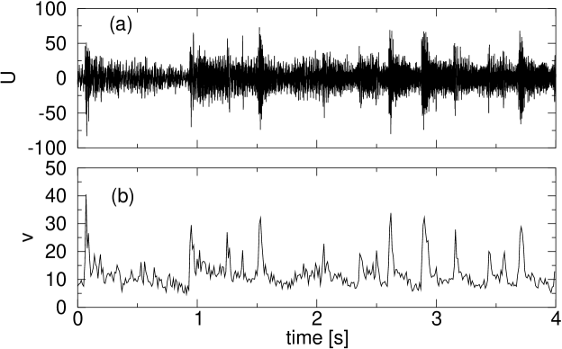
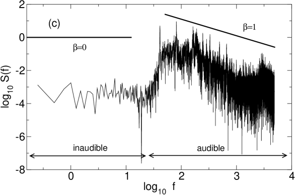
Figure 1: (a) The original signal $U(i)$ and (b) local standard deviation $v(j)$ for a 4 s stretch of music as a function of real time measured in seconds. We can relate the value of $v(j)$ to the instantaneous loudness of the music, as described in the text. (c) double log plot of the power spectrum $S(f)$ as a function of frequency $f$ measured in Hz of $U(i)$. The human ear can only detect monochromatic tones of frequencies in the range $20$ Hz $<f<20$ kHz. We instead perceive frequencies $f<20$ Hz as giving rise to melodic, rhythmic, speech and other such structures that have time scales $t>20^{-1}$ s. Such spectra have previously been studied comprehensively. Note that we find 1/$f$-type behavior for audible frequencies. The spectrum scales approximately as $S(f)\sim f^{-\beta},$ with $\beta\approx 1.$ In contrast, for lower frequencies we find behavior more reminiscent of “white noise,” with $\beta\approx 0.$ Such spectra, while useful for studying power densities in audible frequencies, do not easily adapt to the study of loudness fluctuations. This forms the fundamental basis motivating the development here of a new method that can detect deviations from uniform power law scaling at a given time scale $t$ in the instantaneous loudness of the music.

We now devise methods suitable for studying the scaling properties of the intensity of music signals over a range of times scales [1, 2, 4]. We begin with selected pieces of music taken from CDs and digitize them using 8 bit sampling at $f_{s}=$11 kHz. Since each piece lasts several minutes, therefore, this “low” 11 kHz bit sampling rate suffices for obtaining excellent statistics. Similarly, since we aim not to listen to music, but to study correlations in intensity, 8 bit sound adequately satisfies basic signal-to-noise requirements (better than $100:1$). We choose 4 min stretches of music, and to each piece of music assign a time series $U(i),$ where $0\leq U(i)\leq(2^{8}-1)$ and $i$ represents the sample index (Fig. 1(a)). We generate another series $v(j)$ defined as the standard deviation of every non-overlapping 110 samples of $U(i)$. The variance $[v(j)]^{2}$ thus represents the average intensity of the sound (loudness) over intervals of $0.01$ s (Fig. 1(b)). Concerning the choice of the windowing time interval, we have found the exact value of the time interval to have little or no importance; we have verified that our central results do not depend on the exact value chosen, since we aim to study fluctuations in the intensity of the signal. We have found, e.g., that using a time interval five times larger, $0.05$ s, equivalent to the minimum audible tone frequency of 20 Hz, leads to no significant changes to our main results. In this context, we note that the measurement of the loudness of music has some similarities to the measurement of volatility in financial markets, since in both cases the variance measurement effectively involves a moving window of fixed but arbitrary size [9].

We define the power spectrum $S(k)$ of the signal as the modulus squared of the discrete Fourier transform $\tilde{U}(k)$ of $U(i)$:

$$S(f)\equiv|\tilde{U}(k)|^{2}\;\;,$$ (1)

where $f=f_{s}k=11~{}000\times k$ represents the frequency measured in Hz. At the lowest frequencies, the spectrum appears distorted by artifacts of the fast Fourier transform (FFT) method. Specifically, at small frequencies approaching $1/N,$ where $N$ represents the FFT window size, a spurious contribution arises from the treatment of the data as periodic with period $N$ [17]. The last few decades have seen extensive studies of the audio power spectra, considered nowadays well understood (Fig. 1(c)). The spectral power in the range $20$ Hz $<~{}f~{}<20$ kHz arises due to audible sounds, while lower frequency contributions emerge due to the structure of the music on sub-audible scales larger than 20^-1 s (see Fig. 1(c)).

Since we primarily aim to study loudness fluctuations at these larger time scales $t>20^{-1}$s, we find it more convenient to study the power spectrum $S^{\prime}(f)$ of the series $v(j)$ rather than of the series $U(i).$ This spectrum allows us to study correlations related to loudness at these higher time scales. However, $v(j)$ behaves as a highly nonstationary variable and the power spectrum of nonstationary signals may not converge in a well behaved manner. Therefore, conclusions drawn from such spectra may lead to questions about their validity. In order to circumvent these limitations, we use DFA. Like the power spectrum, DFA can measure two-point correlations in time series, however unlike power spectra, DFA also works with nonstationary signals [10, 11, 13, 14, 18].

The DFA method has been systematically compared with other algorithms for measuring fractal correlations in Ref. [19], and Refs. [13, 14] contain comprehensive studies of DFA. We use the variant of the DFA method described in Ref. [20]. We define the net displacement $y(n)$ of the sequence $v$ by $y(n)\equiv\sum_{j}^{n}v(j)$, which can be thought of graphically as a one-dimensional random walk. We divide the sequence $y(n)$ into a number of overlapping subsequences of length $\tau,$ each shifted with respect to the previous subsequence by a single sample. For each subsequence, we apply linear regression to calculate an interpolated “detrended” walk $y^{\prime}(n)\equiv a+b(n-n_{0}).$ Then we define the “DFA fluctuation” by $F_{D}(\tau)\equiv\sqrt{\langle(\delta y)^{2}\rangle}$, where $\delta y\equiv y(n)-y^{\prime}(n)$, and the angular brackets denote averaging over all points $y(n)$. We use a moving window to obtain better statistics. We define the DFA exponent $\alpha(t)$ by

$$\alpha(t)\equiv\frac{d\log{F_{D}(\tau)}}{d\log{(\tau+3)}}\;\;,$$ (2)

where $t=100~{}\tau$ gives the real time scale measured in seconds. Uncorrelated data give rise to $\alpha=1/2,$ as expected from the central limit theorem, while correlated data give rise to $\alpha\neq 1/2.$ Specifically, a value $\alpha=1/2$ corresponds to uncorrelated white noise, $\alpha=1$ corresponds to $1/f$-type noise with complex nontrivial correlations, and $\alpha=1.5$ corresponds to trivially correlated Brown noise (integrated white noise). Refs. [10, 21] discuss in further detail the relationship between DFA and the power spectrum. A constant value of $\alpha(t)$ indicates stable scaling [10, 11], while departures indicate loss of uniform power law scaling. We obtain the best statistics by studying time scales that range from $10^{-0.5}$ s to $10$ s, hence we focus on these scales.

3 Results

We have recorded 10 tracks from each of 9 genres: music from the Western European Classical Tradition (WECT), North Indian Hindustani music, Javanese Gamelan music, Brazilian popular music, Rock and Roll, Techno-dance music, New Age music, Jazz, and modern “electronic” Forró dance music (with roots in traditional Forró, from Northeast Brazil). We have chosen these genres of music somewhat arbitrarily, noting that our main interest lies not in the music itself but rather in developing quantitative methods of analyzing music that can—in principle—be applied in future studies systematically to compare and contrast diverse audio signals originating in music.

Fig. 2(a) shows the the power spectrum $S^{\prime}(f)$ of the series $v(j).$ As noted previously, $v(j)$ does not have stationarity and therefore the meaning of such spectra may appear ambiguous. Nevertheless, we can observe clear differences in the spectra of each genre of music.

Figs. 2(b,c) show the DFA functions $F_{D}(t)$ and $\alpha(t)$, respectively. Each genre of music has a different $\alpha(t)$ “signature.” In Jazz, Javanese music, New Age music, Hindustani music and Brazilian Pop, $\alpha(t)$ decreases with $t.$ WECT music appears characterized by extremely high $\alpha(t)$ in the region of interest from $10^{-0.5}$ s to $10^{1.0}$ s, with lower values for rock and roll. Techno-dance and Forró music have characteristic $\alpha(t)$ patterns marked by “dips” near 0.8 s. These characteristics also appear in Fig. 3, which shows $\alpha(t)$ for each data set separately.

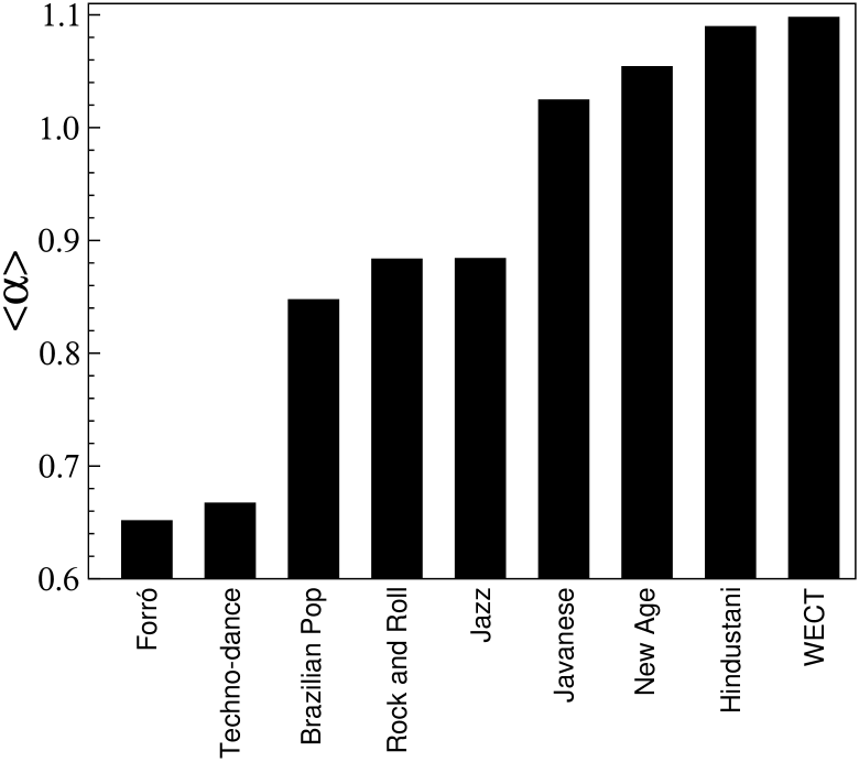
Figure 4: Average values $\langle\alpha\rangle$ for each genre, ranked in increasing order. The standard deviation of the values of $\alpha$ varies from genre to genre, but averages $\Delta\alpha=0.09$. We note the remarkable relationship between $\langle\alpha\rangle$ and the music genre. As discussed in the text, the presence of dominant periodic trends arizing from the regular rhythmic “beats” can lead to lower values of $\langle\alpha\rangle$. The results raise the possibility that the qualitative differences between high art, popular, and dance music genres may be quantifiable.

We also compute the average DFA exponent $\langle\alpha\rangle$ in the region of interest $10^{-0.5}$ s$\leq t\leq 10$ s for each genre of music (Fig. 4). We emphasize that these values of $\alpha$ measure the scaling exponents in the variance—hence, loudness—fluctuations of the music signals. Any conclusions derived from the results presented here must carefully consider this point.

4 Discussion

Javanese Gamelan and New Age, and to a lesser extent Hindustani and WECT, have the values closest to $\langle\alpha\rangle=1$, corresponding to the most complex, nontrivial correlations ($1/f$-type behavior). We note that WECT music has the highest value of $\langle\alpha\rangle,$ indicating that loudness fluctuations have the strongest correlations in this genre. Hence, from the point of view of loudness level changes, WECT music appears the most correlated, and modern electronic Forró music the least correlated. None of the results reported here have a direct bearing on harmony, melody or other aspects of music. Our results apply only to loudness fluctuations, which can reflect aspects of the rhythm of the music [1].

Another observation concerns how the extremely predictable periodic rhythmic structure of Techno-dance music and Forró shows up as minima in $\alpha(t)$ near 0.8 s (Figs. 2(c), 3). This finding suggests that the periodic “beat” of the music, considered abstractly as a superposition of periodic trends and the acoustic signal, leads to significant deviations from uniform power law scaling at that time scale [10, 13, 14].

The above results seem to suggest that the qualitative differences between genres—well known to music lovers—may in fact be quantifiable. For example, WECT music, Hindustani music and Gamelan music, which have the highest average $\langle\alpha\rangle\approx 1$ (suggesting almost perfect $1/f$ scaling behavior), usually belong to the general category of high art music. On the other end, electronic Forró and Techno-dance music, where periodic tends dominate, have the lowest average $\langle\alpha\rangle,$ and arguably belong to the category of dance or danceable music. The lower $\langle\alpha\rangle$ observed in these genres is due to a a bump and horizontal shoulder in the DFA fluctuation fluctation $F_{D}(t)$ that emerges at time scales corresponding to the pronounced periodic beats [13] (see Figs. 2(c), 3). Such genres might have evolved primarily for dancing, rather than for listening. We can speculate from this point of view that Jazz, Rock and Roll, and Brazilian popular music may occupy an intermediary position between high art music and dance music: complex enough to listen to, but periodic and rhythmic enough to dance to.

Finally, we discuss the relevance of these findings to the possible effects of music on the nervous system [24]. Studies of heart rate dynamics using the DFA method have shown that healthy individuals have values relatively close to $\langle\alpha\rangle=1$, corresponding to $1/f$ correlations, while subjects with heart disease have higher values (typically $\langle\alpha\rangle>1.2$) that indicate a significant shift towards less complex behavior in heart rate fluctuations, since $\alpha=1.5$ corresponds to trivially correlated Brown noise (e.g., see [11, 22, 23]). Hence, listening to certain kinds of music may conceivably bestow benefits to the health of the listener [24, 25, 26]. The hypothesis that music with $\langle\alpha\rangle\approx 1$ confers health benefits still requires systematic testing. For example, the so-called “Mozart effect” refers to the conjecture that listening to certain types of music may correlate with higher test scores and more generally to intelligence [24]. If ever such findings become substantiated, then a new approach to the study of music (and perhaps other forms of art) might become a necessity. We note, however, that the Mozart effect has not been legitimately established as a real phenomenon. Nevertheless, the results reported here—and more importantly, the approach used in obtaining the results— point towards the possibility of objectively analyzing subjectively experienced forms of art. Such an approach may find relevance in the academic study of music, and of art in general.

In summary, we have developed a method to study loudness fluctuations in audio signals taken from music. Results obtained using this method show consistent differences between different genres of music. Specifically, dance music and high art music appear at the lower and upper endpoints respectively in the range of observed values of $\langle\alpha\rangle$, with Rock and Roll, Jazz, and other genres appearing in the middle of the range.

   

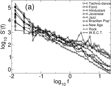
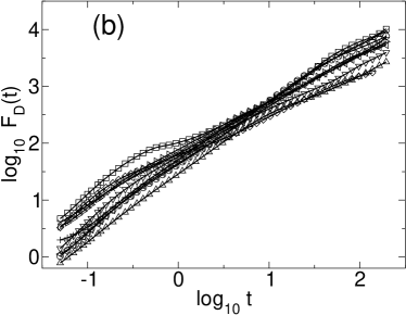
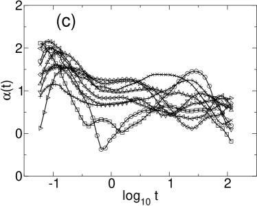
Figure 2: (a) Double log plot of the power spectrum $S^{\prime}(f)$ of the variable $v(j)$ for various genres of music. For every genre we averaged the spectrum for each individual piece of music, found using a windows of size $2^{13}$ samples (corresponding to 81.29 s of music), with shifts of $2^{10}$ samples (10.24s). We applied logarithmic binning to smooth the spectrum by averaging over windows which grow in size as $2^{1/4}.$ These spectra suggest quantitative differences in the scaling properties of the loudness fluctuations that depend on the genre of music. (b) Double log plot of the average DFA functions $F_{D}(t)$ as a function of the time scale $t$ (in seconds) for each genre of music. (c) Log-linear plot of the DFA correlation exponents $\alpha(t)$ obtained from local slopes in (b), according to Eq. 2. Note the striking differences between genres, which also appear in Fig. 3.

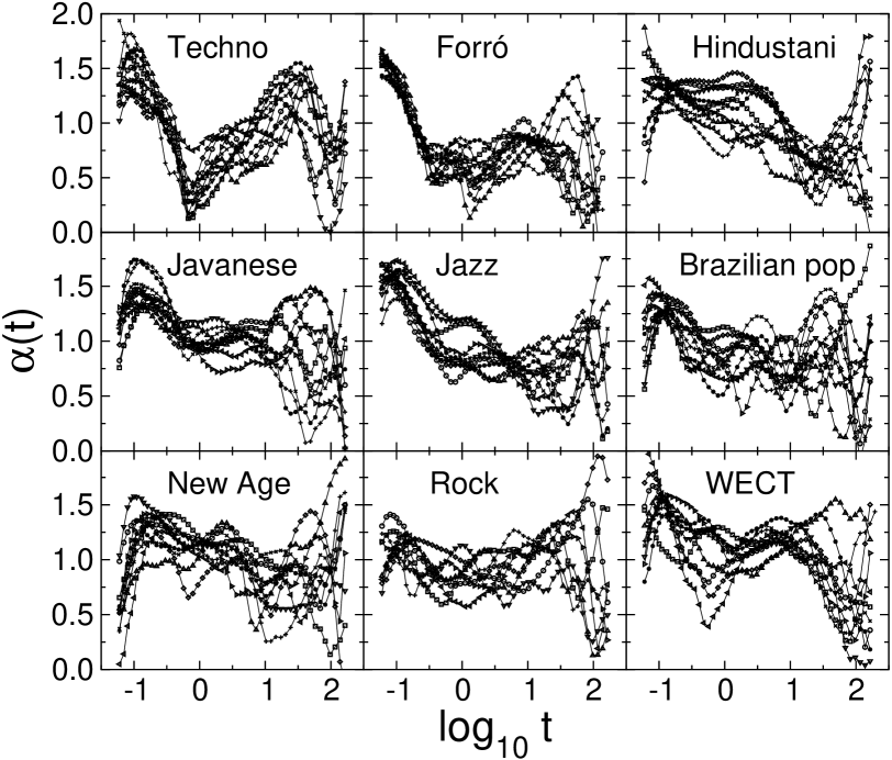
Figure 3: DFA exponents $\alpha(t)$ for 9 genres of music, with 10 representative signals each. We have calculated $\alpha(t)$ according to Eq. 2.

References

- [1] John R. Pierce, in The Psychology of Music, Ed. Diana Deutsch, Academic Press (2nd edition), 1998.
- [2] William M. Siebert, Circuits, Signals, and Systems, The MIT Press, Cambridge, 1986.
- [3] Y. L. Klimontovich and J. P. Boon, Europhys. Lett. 3 (1987) 395.
- [4] R. F. Voss and J. Clarke, Nature 258 (1975) 317.
- [5] M. Dorfler, J. New Mus. Res. 30 (2001) 3.
- [6] J. P Boon and O. Decroly, Chaos 5 (1995) 501.
- [7] K. P. Han et al., Eletronics 44 (1998) 33.
- [8] N. P. M. Todd, G. J. Brown, Artificial Intelligence Review 10 (1996) 253.
- [9] G. M. Viswanathan, U. L. Fulco, M. Lyra and M. Serva, Physica A 329 (2003) 273.
- [10] G. M. Viswanathan, S. V. Buldyrev, S. Havlin and H. E. Stanley, Biophys. Journal 72 (1997) 866.
- [11] G. M. Viswanathan, C.-K. Peng, H. E. Stanley and A. L. Goldberger, Physical Review E 55 (1997) 845.
- [12] C. K. Peng, S. V. Buldyrev, M. Simons, H. E. Stanley and A. L. Goldberger, Phys. Rev. E 49 (1994) 1695.
- [13] K. Hu, Plamen Ch. Ivanov, Zhi Chen, Pedro Carpena and H. E. Stanley, Phys. Rev. E 64 (2001) 011114.
- [14] Zhi Chen, Plamen Ch. Ivanov, Kun Hu and H. E. Stanley, Phys. Rev. E. 65 (2002) 041107.
- [15] B. Truax, Ed., Handbook for Acoustic Ecology [CD-ROM], Vancouver, Cambridge Street Publishing, 2001.
- [16] D. Panter, Modulation, Noise and Spectral Analysis, McGraw-Hill, New York, 1965.
- [17] W. H. Press, B. P. Flannery, S. A. Teukolsky and W. T. Vetterling, Numerical Recipes in C : The Art of Scientific Computing, Cambridge University Press, 1993.
- [18] Jan W. Kantelhardt, Eva Koscielny-Binde, Henio H. A. Rego, Shlomo Havlin and Armin Bunde, Physica A 295 (2001) 441.
- [19] M. S. Taqqu, V. Teverovsky, W. Willinger, Fractals 3 (1995) 785.
- [20] S. V. Buldyrev, A. L. Goldberger, S. Havlin, R. N. Mantegna, M. E. Matsa, C.-K. Peng, M. Simons and H. E. Stanley, Phys. Rev. E 51 (1995) 5084.
- [21] K. Wilson, D. P. Francis, R. Wensel, et al., Physiol. Meas. 23 (2002) 385.
- [22] C.-K. Peng, Shlomo Havlin, H. E. Stanley and A. L. Goldberger, Chaos 5 (1995) 82.
- [23] P. Ch. Ivanov, L. A. N. Amaral, A. L. Goldberger, S. Havlin, M. G. Rosenblum, H. E. Stanley and Z. Struzik, Chaos 11 (2001) 641.
- [24] F. H. Rauscher, G. L. Shaw and K. N. Ky, Nature 365 (1993) 611.
- [25] A. Tornek, T. Field, M. Hernandez-Reif, et al., Psychiatry 66 (2003) 234.
- [26] G. Martin, M. Clarke, C. Pearce, J. Am. Acad. Child. Psy. 32 (1993) 530.