PINNING AND SLIDING OF DRIVEN ELASTIC SYSTEMS:

FROM DOMAIN WALLS TO CHARGE DENSITY WAVES

Abstract

The review is devoted to the theory of collective and local pinning effects in various disordered non-linear driven systems. Common feature of both approaches is the emergence of metastability. Although the emphasis is put on charge and spin density waves and magnetic domain walls, the theory has also applications to flux lines and lattices thereof, dislocation lines, adsorbed mono-layers and related systems. In the first part of the article we focus on the theory of the it collective pinning which includes the equilibrium properties of elastic systems with frozen-in disorder as well as the features close to the dynamic depinning transition enforced by an external driving force. At zero temperature and for adiabatic changes of the force, the dynamic depinning transition is continuous, the correlation length is large, the behavior is dominated by scaling laws with non-trivial static and dynamical critical indices. The application of functional renormalization group methods allows for the detailed description of both equilibrium as well as non-equilibrium properties. The depinning transition is also characterized by the appearance of it new scaling laws. Thermal fluctuations smear out this transition and allow for a creep motion of the elastic objects even at small forces. The application of an ac-driving force also destroys the sharp transition which is replaced by a velocity hysteresis.

The second part of the review is devoted to the picture of the local pinning and its applications. Local theories apply in the region where correlation effects are less important, i.e. not too close to the depinning transition, at low temperatures, at high enough frequencies or velocities. The inclusion of plastic deformations results in a rich cross-over behavior of the force-velocity relation as well as of the frequency dependence of the dynamic response. Being easily affected at higher frequencies or velocities, the local pinning becomes the easily accessed source of dispersion, relaxation and dissipation. The picture of the local pinning can be effectively used to explain experimental data: qualitatively and even quantitatively. The advantages come from the explicit treatment of metastable states, their creation and relaxation, their relation to plasticity and topological defects. The local pinning recovers and exploits new elements of the energy landscape such as termination points of some branches or irreversibility of other ones related to generation of topological defects in the course of sliding. It provides also a clue to quantum effects describing the quantum creep as a tunnelling between retarded and advanced configurations.

ADVANCES in PHYSICS, to be published.

1 Introduction

Many ordering phenomena in solids are connected with the emergence of a modulated structure. Examples are charge or spin density waves [1, 2, 3, 4, 5, 6, 7, 8], Wigner crystals [8, 9], flux line lattices [10, 11], incommensurate phases of adsorbed monolayers [12] etc. These structures often interact with imperfections frozen in the solid leading to pinning phenomena which change drastically the statics and dynamics of the modulated structure.

In other cases topological defects like isolated flux lines in superfluids or superconductors, dislocation lines in solids, domain walls in magnets etc. appear as a result of competing interactions, external fields, or in the process of fabricating the material. Pinning of the motion of these objects is often required if one wants to exploit physical properties of the condensed structure. The pinning of flux lines prevents dissipation from their frictional motion in superconductors, pinning of dislocations prevents plastic deformations of a solid etc.[13, 14, 15]. The generality of this approach has been anticipated already long time ago [16], but strong similarities between different systems mentioned above have been worked out in detail only later on.

The goal of the present article is to give a presentation of unifying concepts in the theory of pinning phenomena. To make the ideas more clear, we will not go too much into the details of specific systems but we shall stress the generality of the approach. Some aspects of pinning have been considered in the past in great detail for type-II superconductors and we refer the reader to these articles for more details [10, 11].

A perfectly rigid object of any dimension, e.g. a straight flux line, a planar domain wall or an undistorted charge density wave will never be pinned – the pinning forces acting on different parts of the object cancel each other. More accurately: the resulting total pinning force is of the order of the square root of the volume of the object. It is therefore necessary to consider the distortions of these objects under the influence of pinning centers which are often of elastic type. We will therefore speak about ”elastic systems” if we refer to arguments which are essentially correct for all systems mentioned above.

The delicate question of pinning by randomness stays already for almost three decades since the earliest proposals of Larkin [17], through theories of vortex lattices [18] and density waves [19, 20, 21]. The last decade has brought new insights, largely provoked by the studies of vortices in high-T_c superconductors [10, 11]. In particular new understanding was reached detecting the possibility of a quasi long-range ordered (Bragg) glass phase with an algebraic decay of structural correlations in a disordered system [22, 23, 24] and by the understanding of the role of metastable states in non-stationary effects. Essential progress was due to new advanced methods like the functional renormalization group method [25, 26] for the collective pinning problem. Still full details are not completely accessible and applications are not always straightforward. The picture of the local or weak pinning was also revised and developed through the last decade in conjunction to plasticity and a role of topological defects.

The undisputable domain of the collective pinning approach are the effects occurring on large length and time scales. These are recovered e.g. in studies of long time evolution, the low frequency response to external forces, the creep below the zero temperature depinning threshold, and the region around the threshold field. The collective or weak pinning forces come from elastic interference of many impurities [18, 21, 20, 19]. Their characteristic features are: large correlation volumes – of the order or beyond the Larkin-length, high energy barriers between metastable states, huge relaxation times and small pinning forces. The collective pinning determines the threshold $f_{c}$ of the driving force to initiate the sliding quite similar to conventional rest friction [27]. The comprehensive picture of the collective pinning will be given in the first part of this review in Sections 2-5.

Complementary insight can be obtained within a frame of the so called strong or local pinning which manipulates with only a few of metastable states. This will be the topic of the second part of this review (Sections 6-12). This simple but transparent approach offers some effects which have not been noticed yet – and still are not fully accessible – within the very complicated picture of the collective pinning. The local or strong pinning comes from rare metastable pinning centers which provide finite barriers, hence reachable relaxation times. Being easily affected at higher frequencies or velocities, the local pinning becomes the easily accessed source of dispersion, relaxation and dissipation. This part will summarize the local pinning approach to time dependent properties of sliding superstructures. We shall follow the scheme of [28, 29, 30, 31] for the theory of the pinning-induced metastable plastic deformations partly due to creation of dislocation loops or lines. Depending on the pinning potential strength, we shall find several regimes of the behavior of local deformations in the course of a displacement with respect to the impurity site. The key observation is that the local state at the pinning center – the impurity – may be either unique or bistable. The bi-stability can be either restricted or unrestricted (i.e. preserved throughout the whole period of sliding). In the latter case this leads to the generation of diverging pairs of dislocation loops – or $2\pi-$ solitons in a quasi 1-dimensional picture. On this basis we can obtain contributions to the pinning force resulting in the sliding velocity-driving force characteristics and in the frequency dependent response.

Special applications will be devoted to the best studied examples of domain walls and CDWs where we shall particularly address two commonly observed experimental features: the totally nonlinear current-voltage curve and the anomalous low frequency low temperature behavior of the dielectric susceptibility.

2 Equilibrium properties of elastic objects in random environments

In this section we summarize the equilibrium properties of elastic objects in a random environment. There are two main classes of systems: The first one refers to non-periodic objects like isolated domain walls, flux or dislocation lines. These can be generalized to the so-called elastic manifolds models. The second class of models is periodic, like charge density waves, flux line lattices or Wigner crystals. These are subsumed under the expression periodic media.

To make the notation simple, we will describe the distortions of the elastic systems from perfect order by a scalar displacement field $u({\bf x})$, its generalization to $N$-vector or more complicated fields is straightforward. Correspondingly we will mostly use the terminology of domain walls and charge density waves, respectively. Where peculiarities in systems with $N>1$ may occur we will mention them however.

2.1 Models

We consider a $D$-dimensional elastic object embedded into a host medium of a dimension $d$. Since the medium includes quenched disorder, the energy can be written in the form

$${\cal H}=\int d^{D}x\left\{\frac{1}{2}C(\mbox{\boldmath$\nabla$}u)^{2}+V_{R}({\bf x},u)-fu\right\}.$$ (1)

Here $D$ denotes the internal dimension of the object ($D=1$ for isolated flux or dislocation lines, $D=d-1$ for isolated domain walls, $D=d$ for charge density waves, flux line lattices and Wigner crystals etc.). Note, that $D$ is in general different from the space dimension $d$ ($D\leq d$). (The dimension $N$ denotes the number of components of the displacement field $u$. For isolated flux lines or domain walls $N=d-D$ whereas for flux line lattices $N=2$ and $N=1$ for CDWs.) $C$ is an elastic constant and in general a tensor, e.g., in flux line lattices at least three elastic constants are necessary for the description. In some cases the elasticity is non-local on intermediate length scales – as for flux line lattices on scales smaller then the London penetration length – or even at all length scales as for dislocation lines. The elastic constants will also show a temperature dependence since they have to vanish at the transition where the structure melts, e.g. at the Peierls transition for CDWs. $f$ denotes an external force density which acts on the object.

The random potential $V_{R}({\bf x},u)$ results from the coupling of the elastic object to the impurity potential $v_{R}({\bf x,z}),\,$ which is generated by the frozen impurities, fluctuating exchange constants etc.:

$$V_{R}({\bf x},u)=\int d^{d-D}z\,v_{R}({\bf x,z})\,\rho({\bf x,z},u)\,,$$ (2)

$\rho({\bf x,z},u)$ represents the density of the elastic object and will be specified below. ${\bf x}=(x_{1},...x_{D})$ and ${\bf z}=(x_{D+1},...,x_{d})$ denote a D- and $(d-D)$-dimensional position vectors parallel and perpendicular to the main orientation of the object (e.g. the domain wall or the flux line), respectively. For density waves and flux line lattices $D=d$ and hence there is no perpendicular coordinate ${\bf z}$.

The average over disorder - which replaces the average over the (infinite) sample - will be denoted $\langle...\rangle_{R}$. Without restricting the generality we will assume that $\langle v_{R}({\bf x,z})\rangle_{R}=0$ – with other words, we incorporate the effect of the averaged disorder potential into the bare parameters of our model and consider only its fluctuations. A less general but still reasonable choice is that ${v_{R}}({\bf x,z})$ is Gaussian distributed and short range correlated (with a correlation length $l$) such that it is characterized by its second moment:

$$\langle v_{R}({\bf x}_{1},{\bf z}_{1})\,v_{R}({\bf x}_{2},{\bf z}_{2})\rangle_{R}=v_{R}^{2}\delta({\bf x}_{1}-{\bf x}_{2})\delta({\bf z}_{1}-{\bf z}_{2}).$$ (3)

If we rewrite the random potential $v_{R}(\mathbf{x},\mathbf{z})$ as a sum of impurity potentials

$$v_{R}(\mathbf{x},\mathbf{z})=\sum\limits_{i=1}^{N_{imp}}V_{i}\delta(\mathbf{x}-\mathbf{x}_{i})\delta(\mathbf{z}-\mathbf{z}_{i})-\bar{V_{i}}n_{imp}$$ (4)

then the disorder average is defined as

$$\big{<}\ldots\big{>}_{R}=\prod\limits_{i=1}^{N_{imp}}\int\frac{d^{D}x_{i}\,d^{d-D}z_{i}}{V}\int\limits_{-\infty}^{\infty}dV_{i}p(V_{i})\ldots$$ (5)

Here $N_{imp}$, $V$ and $n_{imp}$ denote the total number of impurities, the volume of the sample and the impurity concentration, respectively. $p(V_{i})$ is the normalized probability distribution of the potential strength $V_{i}$ with $\overline{V_{i}^{k}}=\int dV_{i}\cdot V_{i}^{k}\cdot p(V_{i})$ and $v_{R}^{2}=\overline{V_{i}^{2}}\,n_{imp}$.

The correlations of the random potential $v_{R}$ are always short ranged provided the impurities are short range correlated. $\delta({\bf x})$, $\delta({\bf z})$ are $\delta$–functions which may be smeared out over a length scale of the order $l$. Since we will use it later we introduce here also the correlation function

$$\langle V_{R}({\bf x}_{1},u_{1})\,V_{R}({\bf x}_{2},u_{2})\rangle_{R}=R({u_{1},u_{2}})\delta({\bf x}_{1}-{\bf x}_{2}).$$ (6)

Because of the gaussian nature of the disorder correlations the disorder averaged physical quantities like the free energy depend only on the correlation function $R({u_{1},u_{2}})$. The relevant contributions of $R({u_{1},u_{2}})$ are those which depend only on the difference $u_{1}-u_{2}$ on which we will concentrate in the following. For $|u|\ll l$, $R(u)$ is quadratic in $u$ (with $R_{uu}(0)<0$), for larger $u$ different cases have to be distinguished (see below).

In the following we consider some specific examples:

(i) Domain walls in magnets : Here $u({\bf x})$ describes the displacement of the domain wall from a planar reference configuration, $D=d-1$ and $N=1$. The stiffness constant $C$ is finite only above the roughening transition temperature $T_{R}$, for $T<T_{R}$ the elastic description breaks down in the absence of disorder. But disorder leads always to roughening of the interface, even at $T=0$ [32, 33, 34]. The driving force density is directly related to the magnetic field $B$ by $f=2\mu_{B}B$. If the random potential results from fluctuations of exchange coupling between the spins (this is the so-called random bond case), which couple only to the domain wall, then $\rho({\bf x},z,u)\sim\delta(z-u({\bf x}))$. In some cases the width of the domain wall may be large compared to the lattice spacing and the $\delta$-function has to be replaced correspondingly by a smeared out profile function. The correlations of $V_{R}({\bf x},u)$ are then short range in ${\bf x}$ and have a correlation length corresponding to the maximum of $l$ and the domain wall width in the $u$-direction. To keep the notation simple we will denote this maximum in the following also by $l$. $R(u)$ is then a $\delta$-function of finite width of the order $\sim l$. The extension of this model to arbitrary $D$ and $N$ (i.e. $D+N$ is not longer equal to $d$) is called the random manifold model.

If disorder comes from random field impurities then the domain wall couples to the disorder in the domains. In this case $\rho({\bf x},z,u)\sim\Theta(u({\bf x})-z)$ which gives the Zeeman energy with a constant magnetization in each domain, $v_{R}({\bf x},z)$ represents now an uncorrelated random magnetic field. In this case of a non-local coupling to the disorder it can be shown that $R(u)\approx-|u|$ for $|u|\gg l$ [35].

(ii) Isolated magnetic flux lines or dislocation lines: $u({\bf x})\to{\bf u}({\bf x})$ denotes now a $N=d-1$ component displacement field and $D=1$. The random potential $V_{R}({\bf x,u})$ is short range correlated both in ${\bf x}$ and ${\bf u}$ and hence $R({\bf u})$ is again a smeared out $\delta$-function. For flux lines, $f$ is given by the Lorentz force ${\bf f}=\frac{1}{c}{\bf j\times{\hat{b}}}\Phi_{0}$, where $\bf j$ denotes the transport current. $\Phi_{0}=hc/2e$ is the flux quantum and $\bf\hat{b}$ the local direction of the magnetic field. In the case of dislocation and vortex lines the elastic energy is non-local [10]. In particular, for dislocation lines one finds after Fourier transformation a weakly momentum dependent elastic modulus $C(k)=-C\log(a_{0}k)$. $a_{0}$ is of the order of the lattice constant. The force acting on the dislocation line is the Peach-Köhler force [36].

(iii) Charge density waves: The condensed charge density can be written as

$$\rho({\bf x},\varphi)=\rho_{0}(1+{\bf Q}^{-1}{\mbox{\boldmath$\nabla$}}\varphi)+\rho_{1}\cos\left({\bf Qx}+\varphi({\bf x})\right)+...$$ (7)

where ${\bf Q}$ denotes the wave vector of the charge density wave modulation and the dots stand for higher harmonics. The first factor describes the density change due to an applied strain. The phase field $\varphi({\bf x})$ is related to a displacement $u({\bf x})$ of the maximum of the density by

$$\varphi({\bf x})=-u({\bf x})Q,$$ (8)

which we will use from now on as the relation between $u$ and $\varphi$.

Since charge density waves carry an electric charge, the stiffness constant $C$ shows in general a strong dispersion due to the long range Coulomb interaction

$$C{\bf k}^{2}\rightarrow C_{\parallel}k_{\parallel}^{2}+C_{\perp}k_{\perp}^{2}+C_{dip}\frac{(k_{\parallel}\lambda/a_{0})^{2}}{1+{\bf k}^{2}\lambda^{2}}\,,$$ (9)

which we will ignore except for special applications. Here $\lambda$ denotes the screening length. If $\lambda$ diverges, the system may be considered effectively as a 4-dimensional one with $k_{\parallel}/k$ playing the role of a fourth dimension [37].

Corresponding to the two $\varphi$-dependent contributions proportional to $\rho_{0}$ and $\rho_{1}$ in (7) there are two contributions in (2) which sometimes are referred to as forward and backward scattering, respectively. The resulting correlator $R(u)$ is periodic in $u=-\varphi/Q$ with the periodicity $2\pi/Q$. Indeed, for charge density waves we obtain from equations (6) and (7)

$$R(\varphi)\propto-\frac{1}{2}\rho_{0}^{2}\big{(}{\bf Q}^{-1}{\bf\nabla}\varphi\big{)}^{2}+\frac{1}{2}\rho_{1}^{2}\cos\varphi.$$ (10)

Here we have neglected strongly oscillating terms (which average to zero) as well as terms which can be included into the elastic energy. Finally, the external force $f$ is given by the applied electric field, $f\sim E$.

For a more detailed discussion of other systems like flux-line lattices, Wigner crystals etc. we refer the reader to the appropriate literature [10, 11, 38, 39, 40].

2.2 Basic properties of disordered systems

To get preliminary information about the influence of disorder on the elastic object and the relevant length scales we consider first small distortions $u({\bf x})$ around the state of perfect order $u({\bf x})\equiv 0$. The energy can then be written as a series expansion in $u({\bf x})$:

$${\cal H}=\int d^{D}x\left\{\frac{1}{2}C(\mbox{\boldmath$\nabla$}u)^{2}+V_{R}({\bf x},0)+V_{R,u}({\bf x},0){u}+\cdots\right\},\quad V_{R,u}=\frac{\partial V_{R}}{\partial u}.$$ (11)

Here we assumed that the distortions are small such that we can neglect for the moment higher order terms in the expansion of $V_{R}({\bf x},u)$.

The necessary condition for the ground state of the Hamiltonian follows from the variation of ${\cal H}$ with respect to ${u}$

$$\frac{\delta{\cal H}}{\delta u}=-C\mbox{\boldmath$\nabla$}^{2}u+V_{R,u}({\bf x},0)=0\,,$$ (12)

which is the Poisson equation known from electrostatics ($u$ and $V_{R,u}({\bf x},0)/C$ playing the role of the electrostatic potential and the charge distribution, respectively).

Its solution is given by

$$u({\bf x})\sim\int d^{D}x^{\prime}\frac{V_{R,u}({\bf x}^{\prime},0)}{C|{\bf x}-{\bf x}^{\prime}|^{D-2}}.$$ (13)

From (13) we obtain with the help of (6)

$$w_{R}^{2}\big{(}|{\bf x}|\big{)}\Big{|}_{T=0}\equiv\left\langle\big{(}u({\bf x})-u({\bf 0})\big{)}^{2}\right\rangle_{R}\sim\frac{(-R_{uu}(0))}{(4-D)C^{2}}|{\bf x}|^{4-D}$$ (14)

where $R_{uu}(0)$ denotes the second derivative of the correlator at $u=0$. At this point we want to mention already one problem with the use of the approximation (12): since the random forces $V_{R,u}({\bf x},0)$ do not depend on $u$, any constant can be added to the solution (13). In other words, the object could be moved through the random environment without any change in energy. Thus the linear approximation misses barriers and metastable states.

As can be seen from (14), the relative displacement in two different points ${\bf 0},{\bf x}$ increases with their separation $|\mathbf{x}|$ below the critical dimension $D_{c}=4$, the elastic object is called to be rough. We can rewrite (14) in a more general form as

$$w_{R}(L)\approx l\left(\frac{L}{L_{p}}\right)^{\zeta}\,,$$ (15)

where we introduce the roughness exponent $\zeta$. In our present calculation $\zeta\equiv\zeta_{\rm RF}=(4-D)/2$, where the subscript RF stands for random force corresponding the expansion of $V_{R}({\bf x},u)$ up to a force term in equation (11). The characteristic length scale $L_{p}$

$$L_{p}\approx\left(\frac{(4-D)l^{2}C^{2}}{|R_{uu}(0)|}\right)^{1/(4-D)}$$ (16)

is called the Larkin–length [17] in the context of flux line lattices, the Fukuyama–Lee length [20] in the context of charge density waves, the Imry–Ma length [41] for random magnets etc.. On this length scale the displacement is of the order of the correlation length $l$ of the random potential, i.e. the displacement field can choose between different energy minima and hence meta-stability appears. For weak disorder, $L_{p}$ is large compared with the mean impurity distance $n_{imp}^{-1/d}$ and hence pinning phenomena arise from the collective action of many impurities. In the situation of strong pinning, which we will discuss further in the second half of this article, individual pinning centers lead to strong distortions already on the scale shorter than the distance between impurities $n_{imp}^{-1/d}$. In the next chapters we will always assume $L_{p}\gg n_{imp}^{-1/d}$. The Larkin-length will then play the role of an effective small-scale cut-off for the phenomena considered in the following.

Unfortunately, the result (14) is not applicable on length scales much larger than $L_{p}$ since equation (12) is only a necessary condition for the ground state: it is the condition for a saddle point, not only for the absolute minimum. It is generally believed that the elastic object has a unique (rough) ground state [42]. But for distortions $u>l$ the system has in general many local minima and perturbative methods break down. A nice demonstration of the breakdown of perturbation theory in systems with several energy minima has been given by Villain and Semeria [43]. In this case more elaborate methods like the renormalization group approach have to be applied. This exceeds the scope of the present short review, but a schematic presentation of the method is given below.

The result of this approach is that the roughness $w(L)$ can still be written in the form (15) but with $\zeta_{RF}$ replaced by a non-trivial roughness exponent $\zeta$ with $0\leq\zeta\leq 1$. (For $\zeta>1$ $\mid\nabla u\mid\sim L^{\zeta-1}$ diverges on large length scales and the elastic approach adopted here breaks down.)

For periodic media, in general, effects of disorder are weaker. In the case of elastic manifolds it may pay off for the elastic object to make a large excursion to find a larger fluctuation in the impurity concentration, which lowers the free energy. On the contrary, for a periodic medium, the distortion has to be at most of the order of the period of the medium to reach a favorable interaction between the impurity and the medium. Hence we expect that periodic systems belong to another universality class with different, smaller exponents. The actual result happened to be more drastic: the roughness exponent $\zeta$ for periodic media is zero corresponding to a logarithmic increase of $w_{R}(L)$ [22, 23, 24, 44] (for further details see Section 2.3).

The average $\langle...\rangle_{T}$ over thermal fluctuations does not change the asymptotic behavior of the correlation function

$$w^{2}_{R}(|{\bf x}|)=\left\langle\langle u({\bf x})-u({\bf 0})\rangle^{2}_{T}\right\rangle_{R}\propto|{\bf x}|^{2\zeta}$$ (17)

which vanishes apparently in the absence of disorder. It is this correlation function which dominates the structural properties of the system. But the temperature will have a drastic effect upon the time dependent properties.

Since we want to consider later on the motion of the elastic object under an external force $f$ it is instructive to characterize the energy landscape the elastic object is exposed to. As a first step we consider changes in the free energy $\mathcal{F}_{R}$ (which depends on a particular configuration of the disorder) by going over to a different disorder configuration. Such new disorder configuration may be created in some cases by applying external forces (compare with equation(87)) or changing the boundary conditions. Sample to sample fluctuations of the free energy of a region of linear extension $L$ are then expected to show also scaling behavior described by a new exponent $\chi$

$$\left\langle\left[\mathcal{F}_{R}(L)-\langle\mathcal{F}_{R}(L)\rangle_{R}\right]^{2}\right\rangle_{R}^{1/2}\approx T_{p}\left(\frac{L}{L_{p}}\right)^{\chi}\equiv{F}(L),\qquad T_{p}=Cl^{2}L_{p}^{D-2},\qquad\chi=D-2+2\zeta.$$ (18)

where $T_{p}$ denotes a characteristic energy scale see e.g. [45, 46, 47, 48]. The scaling relation between $\chi$ and $\zeta$ can be understood from the fact that in the free energy the elastic and the random part of the energy have to be of the same order and therefore it is plausible that the scaling behavior of $\mathcal{F}_{R}(L)$ can be read off from the scaling of the elastic energy, which scales with the exponent $\chi$. An illustrative one–dimensional example of the free energy fluctuations is considered in Appendix A.

Further information about the system comes from a second correlation function $w_{T}(|{\bf x}|)$ which describes the response to a local force which couples to $\big{(}u({\bf x})-u({\bf 0})\big{)}$:

$$w^{2}_{T}(|{\bf x}|)\equiv\left\langle\langle[u({\bf x})-u({\bf 0})]^{2}\rangle_{T}-\langle u({\bf x})-u({\bf 0})\rangle_{T}^{2}\right\rangle_{R}\sim T|{\bf x}|^{2-D}/C+\text{const.}$$ (19)

Any pair correlation function of $u({\bf x})$ can be expressed by a combination of $w_{R}(|{\bf x}|)$ and $w_{T}(|{\bf x}|)$. Equation (19) is (exactly) the same result as in a non-random system and a consequence of a statistical “tilt-symmetry” of the system [49]. Apparently, $w_{T}(|{\bf x}|)$ vanishes at $T=0$. The result (19) can be related to the static susceptibility

$$\chi=\left\langle\frac{\partial}{\partial f}\langle u({\bf 0})\rangle_{T}\right\rangle_{R}=\frac{1}{T}\int d^{D}x\left\langle\langle u({\bf x})u({\bf 0})\rangle_{T}-\langle u({\bf x})\rangle_{T}\langle u({\bf 0})\rangle_{T}\right\rangle_{R}$$ (20)

where $f$ is the force conjugate to $u$.

To discuss the result for $w_{T}(|{\bf x}|)$ further we consider the case when $u(0)$ is fixed to zero such that $w^{2}_{T}(|{\bf x}|)=\left\langle\left\langle(u({\bf x})-\langle u({\bf x})\rangle_{T})^{2}\right\rangle_{T}\right\rangle_{R}\equiv\left\langle\left\langle\delta u^{2}({\bf x})\right\rangle_{T}\right\rangle_{R}$. The quantity $\delta u({\bf x})=u({\bf x})-\langle u({\bf x})\rangle_{T}$ describes the fluctuations of $u({\bf x})$ around its thermal average in a given random environment. Naively one could assume that these fluctuations are restricted to a narrow valley along the ground state such that the fluctuations should not increase with $|{\bf x}|=L$. The result (19) however suggests a different picture: besides of the ground state there are rare excited states which are very different in configuration from the ground state, $\delta u({\bf x})\sim l(L/L_{p})^{\zeta}$, the energy of which differs only by an amount of the order $\Delta E\leq T$ from the ground state (compare with Figure1).

Figure 1: Ground and low energy excited state of a $1D$ domain wall

These excited states could become indeed true ground states if we would change the random potential locally (i.e. in the neighborhood of the initial ground state) in an appropriate manner. Since at $T=0$ the free energy is given by the ground state energy we have to expect that rare excited states differ in energy as the sample to sample variations of the free energy.

To calculate the fluctuations of $\delta u$ we make therefore for the probability distribution of the energy of the excited states of an elastic object of linear extension $L$ the scaling Ansatz

$$P(\Delta E,L)=F^{-1}(L)p(\Delta E/F(L))$$ (21)

where $F(L)$ denotes the sample to sample variations of the free energy (compare with equation (18)) and $p(x)$ is an unknown normalized function with $p(0)=O(1)>0$. With this Ansatz we find for the average fluctuations at low temperatures $T\ll F(L)$ [47, 48]

$$\left\langle|\delta u({\bf x})|^{n}\right\rangle_{T,R}\approx l^{n}\left(\frac{L}{L_{p}}\right)^{n\zeta}\int_{0}^{T}d(\Delta E)\,P(\Delta E,L)\sim l^{n}\frac{T}{T_{p}}\left(\frac{L}{L_{p}}\right)^{n\zeta-\chi}$$ (22)

which gives for $n=2$ the exponent ${n\zeta-\chi}=2-D$ appearing in (19).

The success of this approach gives us the possibility to calculate also the specific heat

$$c(T)=L_{0}^{-D}\frac{\partial}{\partial T}\langle{\Delta E}\rangle_{R}\approx\frac{\partial}{\partial T}\int_{L_{p}}^{\infty}dL\,\nu(L)\int_{0}^{T}d(\Delta E)\cdot\Delta E\cdot P(\Delta E,L).$$ (23)

Here $L_{0}$ and $\nu(L)$ denote the system size and the size distribution of the rare low energy excited states on the scale $L$, respectively. In writing down (23) we have decomposed the system in $(L_{0}/L)^{D}$ blocks of linear extension $L$. Each of them gives a contribution to the internal energy of the order of the integral on the r.h.s. of (23). Then we have to sum over the contributions from all length scales $L$, $L_{p}<L<L_{0}$. The smallest scale is clearly given by the Larkin scale $L_{p}$. The next independent contributions come from excitations on larger scales $bL_{p},b^{2}L_{p},...,b^{n}L_{p}$ etc., $b>1$. ($b$ has to be chosen in such a way that excited states on scale $b^{k+1}L_{p}$ cannot be reached already on scale $b^{k}L_{p}$, which requires $b^{\zeta}\gtrsim 2$.) The total number of scales is given by $\ln(L_{0}/L_{p})/\ln b$. If we replace this sum over $n$ by an integral over $L$, we obtain a factor (the integration measure) $dL(L\ln b)^{-1}(\frac{L_{0}}{L})^{D}$ and hence $\nu(L)\propto\frac{1}{L^{1+D}}$ [50]. (Roughly speaking we could say that we integrate over all momenta $d^{d}k$ with $k\sim L^{-1}$.)

In principle, the distribution $P(\Delta E,L)$ may also depend on the temperature. If we ignore this unknown dependence, we get

$$c(T)\sim\int_{L_{p}}^{\infty}dLL^{-D-1}\frac{T}{F(L)}p\left(\frac{T}{F(L)}\right)\approx\frac{T}{T_{p}}p(0)L_{p}^{\chi}\int_{L_{p}}^{\infty}\frac{dL}{L^{D+1+\chi}}\sim\frac{1}{D+\chi}\frac{T}{T_{p}}L_{p}^{-D}$$ (24)

since the integral is dominated by small $L$ and $p(T/T_{p})\approx p(0)$. This approach gives at $T\ll T_{P}$ a specific heat linear in $T$ which is similar to physics of common two-level systems in amorphous solids [51]. This analogy also builds a bridge to the local pinning picture which thermodynamically is equivalent to the case of [51]. Within the collective picture, similar results have been obtained, in another way, recently in [52]. The precise value of $b$ remains unknown in this approach but has no influence on the temperature dependence. Measurements of the specific heat on a finite time scale $t$ will lead to a reduced value of $c(T)$ since not all local energy minima can be reached by thermally activated hopping. We will give a time dependent correction factor (which takes this fact into account) at the end of Section 3.2.

So far we have considered mainly the case of weak pinning. The large scale properties ($L>L_{p}$) are dominated in this case by density fluctuations of the disorder where many impurities are involved. We want to stress that in the case of strong pinning on very large scales pinning phenomena are again dominated by density fluctuations of the impurities. Strong pinning on small scales is however very different from weak pinning and will be further discussed in the second part of this article. A one–dimensional CDW–model with strong pinning [19, 53] is considered in Appendix B.

2.3 Results from the renormalization group method

In the rest of this section we give a short account of the application of the renormalization group (RNG) [54, 55] approach to elastic systems in random environments [56, 57]. The RNG method starts from a Fourier decomposition of the displacement field $u({\bf x})=\sum_{\bf k}u_{\bf k}e^{-i{\bf k}{\bf x}}$. The first step of the procedure consists in the elimination of the short wave length degrees of freedom $u_{\bf k}^{\phantom{1}}\equiv u_{\bf k}^{>}$ with ${\bf k}$ in the momentum shell $\Lambda_{0}/b\leq|{\bf k}|\leq\Lambda_{0},\;b>1$, from the partition function. $\Lambda_{0}={2\pi}/{a_{0}}$ denotes a microscopic momentum cut–off. The result of taking the trace over $u_{\bf k}^{>}$ can be written again in the form of a Boltzmann factor with a new effective Hamiltonian for the remaining degrees of freedom. If thermal fluctuations are irrelevant, as for $D\geq 2$-dimensional systems, this procedure reduces to the problem of finding the values $u_{\bf k}^{>}=\tilde{u}_{\bf k}^{>}$ which minimize the energy, keeping all $u_{\bf k}^{\phantom{1}}\equiv u_{\bf k}^{<}$ with $|{\bf k}|\leq\Lambda_{0}/b$ fixed. Plugging these values $\tilde{u}_{\bf k}^{>}$ into the Hamiltonian we get the new effective Hamiltonian which contains less degrees of freedom [56]. Since the scale $ba_{0}$ on which the $u_{\bf k}^{>}$ components describe displacements is small, we can expect that there is only one minimum as a solution for $\tilde{u}_{\bf k}^{>}$ such that the application of perturbative methods is allowed. To avoid further misunderstanding we stress here that we always assume in this Section that the system may reach thermal equilibrium, even if the time scales are huge. Besides of corrections to terms already present in the initial Hamiltonian also new terms may be generated in this procedure, their precise form depends on $V_{R}({\bf x},u)$. The concrete implementation of this procedure is in general difficult and rests often on approximations valid close to certain critical dimensions.

The second step of the renormalization group procedure consists in a rescaling of length, time and fields according to

$${\bf x}={\bf x}^{\prime}b,\qquad t=t^{\prime}b^{z},\qquad u({\bf x})=u^{\prime}({\bf x}^{\prime})b^{\zeta}$$ (25)

with so far unspecified dynamical exponent $z$ ($\geq 0$) and roughness exponent $\zeta$ ($\geq 0$). After the first step of the RG-transformation the remaining minimal length scale was $\Delta x_{\rm min}=a_{0}b$ which, after rescaling according to (25), goes over into the original minimal length $\Delta x^{\prime}_{\rm min}=\Delta x_{\rm min}/b=a_{0}$.

Using rescaling (25) in equation (1), the elastic energy in the new coordinates obtains a factor $b^{D-2+2\zeta}$. Since in statistical physics the Hamiltonian appears always in the combination ${\cal H}/T$, we can absorb this factor in a rescaled temperature

$$T^{\prime}=Tb^{2-D-2\zeta}.$$ (26)

The rescaling has also to be applied to the second term in (1). Having introduced $T^{\prime}$, $V_{R}({\bf x},u)$ is replaced by $b^{2-2\zeta}V_{R}\big{(}b{\bf x}^{\prime},u^{\prime}({\bf x}^{\prime})b^{\zeta}\big{)}\equiv V_{R}^{\prime}({\bf x}^{\prime},u^{\prime})$. The correlator of $V_{R}^{\prime}$ is then given by

$$\left\langle V_{R}^{\prime}({\bf x}^{\prime}_{1},u_{1}^{\prime})V_{R}^{\prime}({\bf x}_{2}^{\prime},u_{2}^{\prime})\right\rangle_{R}=b^{4-4\zeta-D}\delta({\bf x}_{1}^{\prime}-{\bf x}_{2}^{\prime})R\left({b^{\zeta}}(u_{1}^{\prime}-u_{2}^{\prime})\right)\,.$$ (27)

As mentioned already, equations (26) and (27) do not represent the whole change of $T$, $R$ under the renormalization, since the new terms produced in the first – non–trivial – step of the procedure will generate contributions to $R^{\prime}$ and $T^{\prime}$. In general the whole function $R(u)$ is transformed in a non–trivial way. We will not discuss here the derivation of this transformation but only present the result. The interested reader is referred to the original articles [25, 26, 56, 57]. For infinitesimal changes of $b=1+\delta b$ one obtains a continuous flow of these quantities. To lowest order in $4-D$ one finds with $\delta b=\delta L/L$:

$$\begin{split}\frac{\partial R(u)}{\partial\ln{L}}&=(4-D-4\zeta)R(u)+\zeta uR_{u}(u)+\frac{1}{2}R_{uu}(u)^{2}-R_{uu}(u)R_{uu}(0),\\ \frac{dT}{d\ln{L}}&=(2-D-2\zeta)T+\ldots\end{split}$$ (28)

where $R_{u}(u)=\frac{\partial}{\partial u}R(u)$ etc. To make the notation easier we have adsorbed here the coefficients of the quadratic terms in $R$ into the redefinition of $R(u)$.

A word of caution seems to be indicated at this point: the rescaling (25) is a matter of convenience, not a physical necessity. If one does not rescale at all, the first step of the renormalization group still keeps the whole information about the large scale behavior of the system. In this case one obtains the effective physical quantities (those which one observes in experiments) on the corresponding length scale $L$.

For systems with uncorrelated disorder ($V_{R}(\mathbf{x},u)$ is a random function of both arguments) there is an important simplification since there is no renormalization of $T$. Indeed, the full stiffness constant $C$ can be measured by replacing the periodic boundary conditions used so far by $u(L,x_{2},...,x_{D})=u(0,x_{2},...,x_{D})+\delta u$, that is applying an overall strain $\frac{\delta u}{L}$ in $x_{1}$–direction. The effective elastic constant $C_{{\emph{eff}}}$ follows then from the free energy $\mathcal{F}_{R}(L,u)$

$$C_{{\emph{eff}}}=L^{-D+2}\partial^{2}\mathcal{F}_{R}(L,u)/\partial\delta u^{2}\,.$$ (29)

The change of the boundary conditions can be compensated by introducing a new variable $\tilde{u}({\bf x})=u({\bf x})-\delta u\,x_{1}/L$. Changing from $u$ to $\tilde{u}$ in the Hamiltonian (1) adds to the elastic energy a constant contribution $\delta{\cal H}=\frac{C}{2}L^{D-2}{\delta u}^{2}$ and changes the random potential into $\int d^{d}xV_{R}({\bf x},\tilde{u}({\bf x})+\delta u\,x_{1}/L)$. Since $V_{R}({\bf x},u)$ is by definition a random function of its arguments, $V_{R}({\bf x},\tilde{u}({\bf x})+\delta u\,x_{1}/L)$ can be replaced by a random potential $\tilde{V}({\bf x},\tilde{u}({\bf x}))$ with the same statistical properties. Thus, the only change in the Hamiltonian is given by the constant $\delta{\cal H}=\delta\mathcal{F}_{R}(L,u)$ from which one concludes with (29) $C_{\emph{eff}}=C$. Since $T$ appears only in the combination $C/T$, there is also no renormalization of $T$.

Figure 2: The $D-N$ plane characterizing different elastic manifolds in a random medium ($\alpha=N$). For $D>4$ weak disorder and for $D>2$ thermal fluctuations are irrelevant. For $4>D>D_{N}$ (i.e. $\lambda_{R}>0$) weak disorder is relevant leading to a non-zero roughness exponent. For $D_{N}>D$ a thermal depinning transition exists: at low temperature weak disorder leads to a non-trivial roughness exponent $\zeta$ whereas in the high temperature phase $\zeta_{T}=(2-D)/2$.

The flow of $R(u)$ and $T$ as given by equation (28) will terminate in stable fixed points (other forms of flow like limit cycles are excluded by general reasons), which characterize physical phases. To find a finite fixed point of the disorder (if it exists) we have to tune the value of the exponent $\zeta$ in order to make elastic and disorder energy scale in the same way. The fixed point condition thus delivers the value of the exponent $\zeta$. Different fixed points have in general different values of $\zeta$. If several fixed points exist – this is the typical situation – the domain of attraction of a fixed point determines the phase boundary. Clearly, the flow close to a fixed point depends on the value of $\zeta$ at this fixed point.

Figure 3: Schematic phase diagrams of impure elastic systems as a function of space dimension for (left) non-periodic media (single flux lines, domain walls) and (right) periodic media (flux line lattices, charge–density waves, Wigner crystals). $v_{R}$ and $T$ denote the strength of the disorder and temperature, respectively. Fixed points characterize the properties of a phase, their domain of attraction ends at the phase boundary. For realistic phase diagrams further degrees of freedom may become relevant (dislocations etc.). In $D\geq 4$ dimensions besides of the fixed point $v_{R}^{\ast}=0$ there may be another strong disorder fixed point.

If there is no disorder, $R\equiv 0$, the roughness exponent is $\zeta=\zeta_{T}\equiv\frac{2-D}{2}$ (for $D\leq 2$) according to (28) and each value of $T$ is a fixed point. Since we exclude negative roughness exponents (there is always a constant contribution to the roughness), we put $\zeta_{T}=0$ for $D>2$ and hence $T$ is transformed to zero. Switching on the disorder only the linear terms in $R$ in equation (28) matter as long as the disorder remains weak. If the initial function $R(u)$ shows a simple power law behavior, $uR_{u}(u)\propto{-\alpha}R(u)$ ($\alpha=-1$ for random field and $\alpha=N$ for random manifold systems, respectively), we get $d\ln R/d\ln L=4-D-\zeta(4+\alpha)\equiv\lambda_{R}(\zeta)$. Using as the initial value for $\zeta$ its value at the thermal fixed point, $\zeta=\zeta_{T}$, we see that the disorder grows provided $4-(4+\alpha)\zeta_{T}-D>0$. To get a new stable fixed point we have to choose then a new value for $\zeta$. In this situation we have to take into account also the nonlinear contributions in equation (28). The resulting fixed point function $R^{*}(u)$, which determines also the value of $\zeta$, depends on the initial function of $R(u)$ and can be found often only numerically [25, 26]. A characteristic feature of the $R^{*}(u)$ is the cusp singularity, $R_{uu}^{*}(u)-R_{uu}^{*}(0)\propto\mid u\mid$ for small $\mid u\mid$, which appears on length scales $L>L_{p}$ and is related to the appearance of metastability (see below).

The true roughness exponent for manifolds in random bond systems can then be written as an expansion in $\epsilon=4-D$. For interfaces in random bond systems one finds $\zeta=0.2083\epsilon+0.0069\epsilon^{2}+O(\epsilon^{3})$ [26, 58]. It has been suggested that $\zeta_{RB}$ can be written in closed form as $\zeta_{RB}=\frac{4-D}{4+N\,\nu(D,N)}$ where $\nu(1,1)=0.5$, $\nu(1,2)=\frac{2}{5}$ and $\nu(1,3)=\frac{8}{21}$ [59, 60].

For random field system $\zeta_{RF}=\frac{4-D}{3}$ for $2<D<4$ [26].

For $\lambda_{R}(\zeta_{T})>0$, $T/C$ is always transformed to zero, thermal fluctuations are irrelevant. In the opposite case $\lambda_{R}(\zeta_{T})<0$ weak disorder is irrelevant. Increasing the disorder strength, there is a phase transition between a disorder dominated phase at low temperatures and a high temperature phase where thermal fluctuations wipe out the disorder. The relation $\lambda_{R}(\zeta_{T})=0$ define the dimension $D(N)$ in Figure2.

The discussion applied so far to the so-called random manifold models, which are given by a non-periodic disorder correlators $R(u)$. For periodic media the correlator $R(u)$ is periodic with period $b$ and this applies also to the fixed point function $R^{*}(u)\sim\left(\frac{1}{36}-\Big{(}\frac{u}{b}\Big{)}^{2}\Big{(}1-\frac{u}{b}\Big{)}^{2}\right)$. However the term $\zeta uR_{u}(u)$ in equation (28) violates the periodicity, from which one has to conclude that for periodic media $\zeta_{pm}=0$ corresponding to a logarithmic increase of the roughness [22, 23, 24, 44, 61]:

$$w^{2}_{R}(L)\sim(4-D)l^{2}\ln{\left(\frac{L}{L_{p}}\right)}\,.$$ (30)

For some applications, e.g. for the calculation of the correlation function $w_{R}(l)$, (but not for studying the effect of energy barriers) one can derive the results for $L>L_{p}$ from the random force model (12) but with a modified correlator for the random forces $V_{R,u}({\bf x})$

$$\langle V_{R,u}({\bf x},0)V_{R,u}({\bf x^{\prime}},0)\rangle_{R}=\int d^{D}ke^{i{\bf k(x-x^{\prime})}}\frac{R_{uu}(0)}{1+\frac{R_{uu}(0)}{R_{uu}^{*}}(kL_{p})^{D-4}}$$ (31)

where $R_{uu}^{*}\propto 4-D$. As can be seen from (31), the force correlations on length scales $L\sim k^{-1}\ll L_{p}$ behaves as $R_{uu}(0)\delta({\bf x}-{\bf x}^{\prime})$ as in the random force approximation of Larkin [17], whereas on length scales $L\sim k^{-1}\gg L_{p}$ there is a long range contribution decaying as $|{\bf x-x^{\prime}}|^{-4}$.

Using the result equation (30) in the structure factor $S({\bf k})$ one obtains a smeared (diffuse) Bragg-peaks of finite width, $S({\bf k})\simeq|{\bf k}-{\bf G}|^{-3+\eta_{\bf G}}$, despite of the fact that the system is dominated by the influence of disorder, hence the name Bragg-glass has been coined [22, 23, 24, 61].

In $D>4$ weak disorder flows to zero, i.e. it is irrelevant, but for sufficiently strong disorder a separate strong disorder fixed point for $R$ may exist. It should be noted that periodic media allow the existence of topological defects like vortices or dislocations which may destroy the Bragg-glass phase. However it can be shown that for weak enough disorder this phase survives in $d=3$ dimensions [62, 63, 64, 65, 66].

In $D=2$ the $T$–axis ($R=0$) is a line of fixed points corresponding to $\zeta=0$. For random manifolds disorder is always relevant, i.e. $\zeta>0$ and there is a non–trivial fixed point at $T^{\ast}=0$, $R^{\ast}>0$ (see the left side of Figure 3). For periodic media (like flux line lattices in a thin film or Wigner crystals) the situation is more complicated: there are two phases both with $\zeta=0$ separated by a phase transition at $T=T_{g}$ (see the right side of Figure 3). In the high–temperature phase

$$w^{2}(L)\sim\frac{T}{C}\ln{\left(\frac{L}{\xi}\right)}\,,$$ (32)

where as in the low–temperature phase ($T<T_{g}$)

$$w^{2}(L)\sim\left(\frac{T_{g}-T}{T_{g}}\right)^{2}\left[\ln{\left(\frac{L}{L_{p}}\right)}\right]^{2}\,.$$ (33)

with the glass temperature $T_{g}\sim C$. The corresponding renormalization group flow diagrams for random manifolds and periodic media in a random matrix are shown in Figure 3.

In $D=1$ dimension the roughness exponent for periodic media is $\zeta=1/2$ both at zero and non-zero temperature [67, 68] (compare Appendix B).

2.4 Metastability

The most important feature of pinning is the appearance of metastability. To demonstrate, how metastability appears for weak pinning on the Larkin scale, we consider here a $D=1$-dimensional example. Let us assume that the renormalization group transformation has been performed $n$ times until the Larkin scale $L_{p}=a_{0}b^{n}$ is reached. Below this scale the perturbation theory is known to be valid and there is no problem in deriving an effective Hamiltonian on this length scale.

The latter can then be written as

$${\cal H}^{(n)}=\sum_{i}^{N}\bigg{\{}\frac{C^{(n)}}{2}(u_{i+1}-u_{i})^{2}+V_{R}^{(n)}(i,u_{i})\bigg{\}}$$ (34)

$C^{(n)}$ and $V_{R}^{(n)}(i,u_{i})$ are the stiffness constant and the random potential on scale $L_{p}$ and the $u_{i}$ are the remaining degrees of freedom. By definition of the Larkin scale the elastic and the random part of the energy are of the same order of magnitude. In continuing the real space RNG we eliminate now half of the degrees of freedom by minimizing the total Hamiltonian, keeping every second $u_{i}$ (say with $i$ even) fixed. This leads to a new effective Hamiltonian

$${\cal H}^{(n+1)}=\sum_{i=2m}\bigg{\{}\frac{C^{(n)}}{4}(u_{i}-u_{i+2})^{2}+V_{R}^{(n)}(i,u_{i})+\delta V_{R}^{(n+1)}\left(i,\frac{u_{i}+u_{i+2}}{2}\right)\bigg{\}}\,,$$ (35)

where

$$\delta V_{R}^{(n+1)}(i,u)=\min_{u_{i+1}}\left[C^{(n)}(u-u_{i+1})^{2}+V_{R}^{(n)}(i+1,u_{i+1})\right].$$ (36)

Figure 4: Left: The two contributions to the potential $\delta V_{R}^{(n+1)}(i,u)$ as well as their derivatives. The points of intersection in the lower figure correspond to local minima of the potential. Note that on scales $L\ll L_{p}$, where the elastic energy is much larger than the random potential, there is only one point of intersection and the derivative of the effective potential is continuous. On the contrary, for $L\gg L_{p}$ more and more meta stable states appear.
Right: The effective potential of $\delta V_{R}^{(n+1)}(i,u)$ as a function of $u$. The potential exhibits random jumps of its derivatives.

The expression in $[...]$ consists of a parabolic potential with the minimum at $u_{i+1}=u$ plus a random potential. Since both are of the same order of magnitude, there will be in general several local minima (compare with Figure 4). Let us start in a situation where $u=0$ and $u_{i+1}=u_{(1)}$ is the true minimum of this expression. Besides of this minimum in general several other local minima at $u_{i+1}=u_{(m>1)}$ will exist. If we change the external variable $u$ to values different from zero, the minimum $u_{(1)}$ may remain for small values of $u$ still the global minimum, but eventually for $u=u_{c}$ another minimum $u_{i+1}=u_{(m)}$ will take over the role of the global minimum. At this point the effective potential $\delta V_{R}^{(n+1)}(i,u)$ is smooth, but the derivative jumps by an amount

$$2C^{(n)}(u_{(1)}-u_{(m)})+V_{R,u}^{(n)}(i+1,u_{(m)})-V_{R,u}^{(n)}(i+1,u_{(1)}).$$ (37)

As a result, the potential shows a cusp at $u=u_{c}$. Since the magnitude and the positions $u_{c}$ of the jumps of the forces are random, the effective potential acting on the degrees of freedom on scales $L>L_{p}$ is scalloped as shown in Figure 4. Continuing this procedure by eliminating further degrees of freedom we will obtain more of those cusps on larger and larger length scales. Such a picture was advocated in [56, 57]; we will demonstrate in the Section 12 its derivation within the local pinning picture. The forces generated by this effective potential $V^{\emph{eff}}_{R}(i,u)$ change continuously between two cusps where they jump from negative to positive values. The typical distance between two consecutive cusps is of the order $l$ since cusps first occur at the Larkin scales. On scales larger than $l$ the forces undergo a random walk such that

$$\big{\langle}\big{(}V^{\emph{eff}}_{R,u}(i,u)-V^{\emph{eff}}_{R,u}(i,u^{\prime})\big{)}^{2}\big{\rangle}_{R}\propto\mid u-u^{\prime}\mid$$ (38)

for small $|u-u^{\prime}|$. This structure of the force correlator is in agreement with our RNG analysis. Indeed, since $-R_{uu}(u)$ is the correlator of forces separated by a distance $u$, the difference $2(R^{*}_{uu}(u)-R^{*}_{uu}(0))\propto-\mid u\mid$ denotes the square of the difference of these forces averaged over the disorder. It has therefore the same meaning and the same random walk property as the quantity in equation (38) [56, 57].

So far we discussed the equilibrium, assuming an adiabatic change of $u$. If we change however $u$ fast enough, the system may not reach equilibrium and remain in the local minimum $u_{(1)}$ until this minimum disappears completely or it may jump to the new minimum with some delay. Such a situation will be considered in the second part of this review when we consider the dynamics of strong pinning.

3 The close to equilibrium motion of elastic objects under an external dc- and ac-drive

In this Section we want to consider the creep motion of the elastic object in a random environment under the influence of a weak external driving force density, $f\ll f_{p}$, where $f_{p}=T_{p}/lL_{p}^{D}$. ($f_{p}$ is of the order of the zero temperature depinning threshold $f_{c}$ discussed in the next Section.) We are now in a non–equilibrium situation which requires its own treatment. If $f$ is however small, as we will assume in this Section, we are sufficiently close to the equilibrium such that we can still use our findings of the previous Section (for earlier descriptions of relaxation phenomena in CDWs see e.g. reference [69]).

3.1 Constant driving force

We first consider the case of a constant driving force $f$. All changes in $f$ are assumed to be made adiabatically. The equation of motion will be assumed to be overdamped with a bare mobility $\gamma$

$$\frac{1}{\gamma}\frac{\partial u}{\partial t}=-\frac{\delta{\cal H}}{\delta u}+\eta({\bf x},t)=C\mbox{\boldmath$\nabla$}^{2}u-V_{R,u}({\bf x},u)+f+\eta({\bf x},t)$$ (39)

where $\eta({\bf x},t)$ denotes the thermal noise

$$\langle\eta({\bf x},t)\eta({\bf x}^{\prime},t^{\prime})\rangle_{T}=2\frac{T}{\gamma}\delta({\bf x}-{\bf x}^{\prime})\delta(t-t^{\prime})\,.$$ (40)

In the following we will repeatedly consider the elastic object on a variable length scale $L$ which may vary from the microscopic cut–off $a_{0}$ to the system size $L_{0}$. The coupling between different length scales due to the anharmonic random potential in (1) is at least partially incorporated into these considerations by (i) the use of the non–mean field exponents $\zeta$ and $\chi=D-2+2\zeta$ and (ii) the condition, that in order to have a moving elastic object on scale $L$, the system has to be able to move on all length scales below $L$. From the dynamical point of view our present analysis is a type of a mean-field treatment.

As follows from equations (18), the typical free energy fluctuations on the scale $L$ are of the order $F(L)=T_{p}(L/L_{p})^{\chi}$. The energy barriers between different metastable states scale as $E_{B}(L)\approx T_{p}(L/L_{p})^{\psi}$ with an exponent ${\psi}$ which is in general different from $\chi$. In the following we will however assume that ${\psi}=\chi$. For some systems this can be shown explicitly (see e.g. [70, 71]). In general this is not the case. A counter example is a system with an additional isolated potential peak $V_{p}\delta({\bf x}-{\bf x}_{0})\delta(u)$, which forms a barrier which can never be overcome by thermally activated hopping (unless we give up the elastic approximation and include topological defects in the structure under consideration). In equilibrium statistical mechanics, however, this potential peak does not play a role, since it can easily be avoided by the elastic object. This example directs us to the picture of the local pinning considered in the Sec. 6 and later on.

Next we include a small driving force density $f$. Taking into account that the typical distance between different metastable states is of the order $w(L)$ (see Figure 1), we can write for the expression of the total energy barrier

$$E_{B}(L,f)\approx F(L)-fL^{D}w_{R}(L)=T_{p}\left(\frac{L}{L_{p}}\right)^{\chi}\left(1-\left(\frac{L}{L_{f}}\right)^{2-\zeta}\right)\,.$$ (41)

The second term on the rhs of equation (41), $-fL^{D}w_{R}(L)$, describes the reduction of the barrier due to the tilt of the potential by the external force $fL^{D}$. In rewriting this term we used (15) and (16) and introduced the force length scale $L_{f}$ associated with the equilibrium length scale $L_{p}$:

$$L_{f}=L_{p}\left(\frac{f_{p}}{f}\right)^{1/(2-\zeta)}\,,\quad f_{p}=\frac{T_{p}}{lL_{p}^{D}}=ClL_{p}^{-2}\,.$$ (42)

$E_{B}(L,f)$ is shown in Figure 5, it has a maximum at $L=\tilde{L}_{f}=L_{f}(\frac{\chi}{\chi+2-\zeta})^{1/(2-\zeta)}<L_{f}$ and vanishes for $L=L_{f}$. Applying a small driving force $f$ corresponds to testing the system on a large length scale $L_{f}$. Note, that $E_{B}(L=L_{p},f)=T_{p}\big{[}1-(f/f_{p})\big{]}$.

Figure 5: Energy barrier as a function of the length scale $L$ for a given driving force density $f$. The different lengths and energy scales are explained in the text.

Assuming for the moment that (41), (42) are valid up to $f\sim f_{p}$, we see that $f\approx f_{p}$ determines the depinning threshold then there is no energy barrier left in the system. Note however that we derived (41) under the condition $f\ll f_{p}$, the vicinity $f\sim f_{p}$ requires a special treatment which we will consider in the following Section.

For $f\ll f_{p}$ the elastic object is restricted in its motion by energy barriers of maximal height

$$\tilde{E}_{B}(f)\equiv E_{B}(\tilde{L}_{f},f)\approx T_{p}\left(\frac{f_{p}}{f}\right)^{\mu}\,,\quad\mu=\frac{\chi}{2-\zeta}\,,$$ (43)

which can be only overcome by thermally activated hopping. The creep velocity of the elastic object follows from $v_{creep}\approx w(\tilde{L}_{f})/\tau(\tilde{L}_{f})$ where we use the Arrhenius law for the hopping time $\tau\sim\omega_{p}^{-1}e^{\tilde{E}_{B}(f)/T}$ and $\omega_{p}\approx C\gamma/L_{p}^{2}=\gamma f_{p}/l$. This results in a creep velocity

$$v(f)\approx\frac{w(\tilde{L}_{f})}{\tau(\tilde{L}_{f})}\propto e^{-\frac{T_{p}}{T}\big{(}\frac{f_{p}}{f}\big{)}^{\mu}}\,.$$ (44)

We omitted the prefactor on the r.h.s. which is beyond the accuracy of the present considerations. This formula is valid for $T\ll\tilde{E}_{B}(f)$ and was found first by Ioffe and Vinokur [72] (see also [73]). Equation (44) was derived from a renormalization group treatment in [74, 75]. In the opposite case $T\gg\tilde{E}_{B}(f)$ we expect a linear relation between the driving force and the velocity:

$$v\simeq\gamma f.$$ (45)

The border line between the two cases, $T\approx\tilde{E}_{B}(f)$, defines a temperature dependent force $f_{T}$

$$f_{T}=f_{p}\left(\frac{T_{p}}{T}\right)^{1/\mu}\,.$$ (46)

Note that the creep formula is valid only for $f\ll f_{T}$, i.e. for $f\ll f_{p}$ and $T\ll T_{p}$.

3.2 Periodically oscillating driving force

Next we consider the motion under influence of an ac driving force with a finite frequency $\omega\ll\omega_{p}=\gamma f_{p}/l$

$$f(t)=f_{0}\sin{(\omega t)}\,.$$ (47)

From the Arrhenius law we conclude that in driving the system over the period of time $\pi/\omega$ only barriers of maximal height $E_{\omega}(T)$ on a corresponding length scale $L_{\omega}$ given by (compare Figure 5):

$$\frac{1}{\omega}\omega_{p}e^{-E_{\omega}(T)/T}\approx 1\qquad\text{i.e.}\qquad E_{\omega}(T)\equiv T_{p}\left(\frac{L_{\omega}}{L_{p}}\right)^{\chi}=T\ln{\left(\frac{\omega_{p}}{\omega}\right)}$$ (48)

can be overcome. If $E_{\omega}(T)>\tilde{E}_{B}(f)$, the oscillating force has enough time to trigger jumps over all relevant barriers and hence the creep formula (44) is still valid (with $f$ replaced by equation (47)). In the opposite limit this is not longer the case and hence there is no global motion, $v\equiv 0$. The relation $E_{\omega}(T)=\tilde{E}_{B}(f)$ determines a temperature and frequency dependent cross–over force $f_{\omega}(T)$

$$f_{\omega}(T)\approx f_{p}\left(\frac{T_{p}}{T\ln{\left(\frac{\omega_{p}}{\omega}\right)}}\right)^{1/\mu}\approx f_{T}\left(\ln{\left(\frac{\omega_{p}}{\omega}\right)}\right)^{-1/\mu},$$ (49)

which separates the creep region $f_{\omega}<f\ll f_{T}$ from the region $f<f_{\omega}$ where $v\equiv 0$. The crossover lines $f_{T}$ and $f_{\omega}$ are depicted in Figure 6. For a discussion of the region $f\approx f_{p}$ see Section 4.

For $f<f_{\omega}$ the elastic object as a whole cannot follow the rapidly oscillating external driving field. However there is still a local motion of parts of the elastic object corresponding to length scales

$$L<L_{\omega}=L_{p}\left(\frac{T}{T_{p}}\ln{\frac{\omega_{p}}{\omega}}\right)^{1/\chi}$$ (50)

(see Figure 5). We consider to this point in the next Section where we will treat these fluctuating parts as two–level systems. As a side remark we note that for similar reasons the specific heat obtains, if measured over a time scale $t$, an extra factor $\left[1-\left(\frac{T}{T_{p}}\ln\omega_{p}t\right)^{-(D+\chi)/\chi}\right]>0$ on the r.h.s. of equation (24).

Figure 6: The cross-over fields $f_{T}$ and $f_{\omega}(T)$ as a function of temperature. Note that for $\omega\to 0$ $f_{\omega}$ approaches the $T$– and $f$–axis, respectively. For $f_{\omega}<f<f_{T}$ the elastic object follows the external field in a creep like motion whereas for $f<f_{\omega}$ only segments of elastic object of size $L<L_{\omega}(T)$ (defined in (48)) can follow the field and the average velocity of the whole object vanishes.

3.3 Dynamic response of the pinned elastic object: Two-level systems

In this subsection we consider the influence of an external time–dependent field $f(t)=f\sin\omega t$ on a pinned elastic object in the region $f\ll f_{\omega}$. Thermal motion over energy barriers $E_{B}(L<L_{\omega})$ mediates transitions between configurations which have an energy difference $\Delta E\lesssim T$. As we discussed already in Section 2.3, the distribution $P(\Delta E,L)$ of $\Delta E$ is smooth and has a width of order $F(L)=T_{p}(L/L_{p})^{\chi}$. Hence there are only rare pairs of metastable configurations with $\Delta E\leq T$. We therefore model the object as an ensemble of noninteracting two–level systems [72, 50].

In the following we discuss the dissipation in a two-level system due to an applied ac-field. We begin with a discussion of a given two-level systems on length scale $L$. The separation between the two minima is $w\sim w(L)$ and the energy difference is $\Delta E$. Then the probability that in thermal equilibrium the system is in the higher–energy minimum is

$$n_{0}(\Delta E)=\frac{e^{-\Delta E/T}}{1+e^{-\Delta E/T}}=\big{[}\exp{(\Delta E/T)}+1\big{]}^{-1}\,.$$ (51)

The external field $f(t)$ disturbs the energy difference $\Delta E$ by $\delta E(t,L)\approx f(t)L^{D}w_{R}(L)$. Therefore the system relaxes to the new time–dependent equilibrium configuration $n(\Delta E+\delta E)\approx n_{0}(\Delta E)+\delta n(t)$. The time dependence of $\delta n$ is controlled by the relaxation time

$$\tau(L)\approx\omega_{p}^{-1}\exp{\big{(}E_{B}(L)/T\big{)}},\qquad\omega_{p}\approx C\gamma/L_{p}^{2}=\gamma f_{p}/l$$ (52)

of the two-level system and by the time dependence of $\delta E(t,L)$. In a linear approximation the time dependence of $\delta n(t)$ is therefore described by the equation

$$\left[\frac{\partial}{\partial t}+\frac{1}{\tau}\right]\delta n+\frac{\partial n_{0}}{\partial\Delta E}\frac{\partial\delta E}{\partial t}=0\,.$$ (53)

The power dissipated in this way by the two-level system of linear size $L$ is given by

$${\cal W}(L,\omega)\sim-Re\left\langle\delta n^{\ast}L^{D}w_{R}(L)\frac{df}{dt}\right\rangle_{\omega}\,,$$ (54)

where $Re\langle...\rangle_{\omega}$ denotes the real part of the Fourier transform. With this and the Fourier transform of equation (53), we get the power absorbed by the given two-level system:

$${\cal W}(L,\omega)\sim\frac{1}{4T}\left[\cosh{\left(\frac{\Delta E}{2T}\right)}\right]^{-2}(\delta E(t,L))^{2}\frac{\omega^{2}\tau}{1+\omega^{2}\tau^{2}}\,,$$ (55)

where $\delta E=fL^{D}w_{R}(L)$. To get the power dissipated by all two-level systems on scale $L...L+\delta L$ we have to average this expression with $P(\Delta E,L)$, equation(21), and multiply it with density $\nu(L)dL\approx\frac{dL}{L^{D+1}}$ (compare with equation (23)) of the two-level systems on scale $L$. Since the distribution function for the $\Delta E$ is smooth and has a width of the order $F(L)\gg T$, only the fraction $T/F(L)$ of them contributes to the average. Hence we obtain for the total power density dissipated by all two-level systems

$${\cal W}_{total}(\omega) \sim \int_{L_{p}}^{\infty}dL\,\nu(L)\int_{0}^{\infty}d(\Delta E)P(\Delta E,L){\cal W}(L,\omega)$$ (56)

$$\approx \int_{L_{p}}^{\infty}\frac{dL}{L}\left(\frac{1}{L}\right)^{D}\frac{\delta E^{2}(L)}{F(L)}\frac{\omega^{2}\tau(L)}{1+\omega^{2}\tau^{2}(L)}$$

The energy dissipation ${\cal W}(L,\omega)$ is related to the imaginary part of the dynamic susceptibility

$$\chi(L=2\pi/\mid{\bf k}\mid,T,\omega)\sim\int d(t-t^{\prime})e^{i\omega(t-t^{\prime})}\langle\langle\partial u_{\bf k}(t)/\partial f_{-\bf k}(t^{\prime})\rangle_{T}\rangle_{R}$$ (57)

$${\cal W}(L,\omega)\sim\frac{1}{2}\omega\chi^{\prime\prime}(L,T,\omega)f^{2}\,.$$ (58)

The total susceptibility is given by the integral over $L$ with the probability distribution $\nu(L)dL$ similarly to (56). The main contribution to the real par $\chi^{\prime}(\omega)$ comes from the length scale $L$ which fulfills the condition $\partial\chi^{\prime}(L,\omega)/\partial L=0$. This yields $(\omega\tau)^{-2}\approx\big{[}\chi E_{B}(L)/T-1\big{]}$. For low frequencies and temperatures this gives $L\approx L_{\omega}$ (compare with equation (50)) and hence

$$\chi^{\prime}(T,\omega)\sim\int dL\nu(L)P\big{(}\Delta E(L),L\big{)}\chi^{\prime}(L,T,\omega)\approx\frac{L_{p}^{2}}{C}\left[\frac{T}{T_{p}}\ln{(\frac{\omega_{p}}{\omega})}\right]^{2/\chi}.$$ (59)

Decreasing the frequency leads to an increase of the susceptibility which is a typical experimental trend, as well as the logarithmic dependence on the frequency $\omega$.

4 Critical Depinning at $T=0$

4.1 Constant driving force, $f\geq f_{c}$

So far we considered the region $f\ll f_{p}$. Increasing $f$ we expect to reach a critical force density $f_{c}$ (as it turns out it is of the order of $f_{p}$) at which the elastic object is depinned. Above the depinning transition the elastic object moves even without the help of thermal activation with a finite velocity $v$ which reaches the non-critical regime $v\approx\gamma f$ at large driving forces $f$. Qualitatively the $v-f$ diagram is depicted in Figure 7.

Figure 7: The velocity of the driven elastic object as a function of the driving force $f$ both at zero and non-zero temperatures.

All changes in $f$ are again to be performed adiabatically. The equation of motion in the absence of thermal fluctuations reads

$$\frac{1}{\gamma}\frac{\partial u}{\partial t}=C{\bf\nabla}^{2}u+f+g({\bf x},u)=-\frac{\delta{\cal H}}{\delta u}\,.$$ (60)

Here we introduced the pinning force density

$$g({\bf x},u)\equiv-V_{R,u}({\bf x},u)\equiv-\frac{\partial V_{R}}{\partial u}$$ (61)

resulting from the random potential. It is also Gaussian distributed with the correlator

$$\langle g({\bf x},u)g({\bf x^{\prime}},u^{\prime})\rangle_{R}=\delta({\bf x}-{\bf x^{\prime}})\Delta(u-u^{\prime}),\quad\Delta(u)=-R_{uu}(u)\equiv-\frac{\partial^{2}R}{\partial u^{2}}$$ (62)

for the bare (unrenormalized) correlators. If the object is completely stiff, i.e. $u({\bf x},t)\equiv u(t)$, – this is the situation if $L_{0}\ll L_{p}$, –, then the average pinning force density $\langle g({\bf x},u)\rangle_{R}$ vanishes and its fluctuations are of the order $(L_{0}^{-D}\Delta(0))^{1/2}$ and hence arbitrarily small for a macroscopic object. Thus a rigid object would never be pinned.

Next we shall use perturbation theory for weakly distorted elastic objects [18, 21]. To this aim it is convenient to go over to a co-moving frame by rewriting $u({\bf x},t)=vt+\tilde{u}({\bf x},t)$ with $\langle\tilde{u}\rangle_{R}=0$ and look for the lowest non-zero correction to the velocity. Indeed such an approach works well at high velocities where the displacements $\tilde{u}$ are small. This gives

$$\gamma^{-1}v-f=\langle g({\bf x},vt+\tilde{u}({\bf x},t))\rangle_{R}\approx\langle g_{u}({\bf x},vt)\tilde{u}({\bf x},t)\rangle_{R}$$ (63)

where $g_{u}({\bf x},u)=\partial g({\bf x},u)/\partial u$. In the lowest order perturbation theory

$$\tilde{u}({\bf x},t) = \int d^{D}x^{\prime}\int_{-\infty}^{t}dt^{\prime}G_{0}({\bf x}-{\bf x}^{\prime},t-t^{\prime})g({\bf x}^{\prime},vt^{\prime}),$$ (64)

$$G_{0}({\bf x},t) = \gamma\int_{\bf k}e^{i\bf{kx}}e^{-C\gamma{\bf k^{2}}t}$$

and with the help of (62), we get from the r.h.s. of equation (63)

$$\gamma^{-1}v-f=(4\pi C)^{-D/2}\int_{(C\Lambda^{2})^{-1}}^{\infty}d\tau\tau^{-D/2}\Delta_{u}(v\tau/\gamma)$$ (65)

The large scale momentum cut–off $\Lambda\sim a_{0}^{-1}$ appearing in (64) was taken into account by adding a factor $e^{-k^{2}/\Lambda^{2}}$. Moreover, we introduced $\tau=t\gamma$ as a new variable. We imply here that $D>2$ and hence the integral (65) is convergent at large $\tau$. Below we will see that this restriction is unnecessary. Decreasing $f$ and hence $v$, one finds for $v\rightarrow 0+$ a non-zero threshold $f_{c}$ if and only if $\Delta_{u}(0+)$ is non-zero:

$$f_{c}\sim-\frac{\Delta_{u}(0+)\Lambda^{D-2}}{(D-2)C}$$ (66)

The result (66) looks at a first glance different from $f_{p}\approx ClL_{p}^{-2}$ which we found in the previous Section. Most importantly, the correlator $\Delta(u)=-\Delta(-u)$ of the random forces has to have a cusp-like singularity at the origin since $-\Delta_{u}(0+)=\Delta_{u}(0-)$ has to be positive. This is not what one gets naively from a weak random potential $V_{R}({\bf x},u)$ which shows an analytic behavior of $\Delta(u)$ for small $u$ and hence $\Delta_{u}(0+)=0$.

This long standing problem has been overcome by the renormalization group theory of critical depinning at $T=0$ [76, 77, 78, 79, 58]. It was shown that the force-force correlator $\Delta(u)$ develops indeed a cusp-like singularity on scales $L>L_{p}$ after the degrees of freedom on scales $L<L_{p}$ have been integrated out. To lowest order in $\epsilon=4-D$ the renormalization group equation for $\Delta(u)$ in this non-equilibrium situation is identical to that for $-R_{uu}(u)$ following from equation (28) (calculated under equilibrium conditions) by differentiating $R(u)$ twice with respect to $u$. Note that this simple relation breaks down to order $\epsilon^{2}$ [58]. Hence $\Delta_{u}(u\to 0)\neq 0$. The force correlator on these scales becomes scale dependent and reads

$$\Delta(u)\rightarrow\Delta(u;L)\propto(Cl/L_{p}^{\tilde{\zeta}})^{2}L^{-4+D+2\tilde{\zeta}}\Delta^{*}\left(u(L/L_{p})^{-\tilde{\zeta}}/l\right),$$ (67)

where the function $\Delta^{*}(y)$ has a cusp for small $y$. Similarly, the mobility $\gamma$ is replaced by an effective scale dependent expression

$$\gamma\rightarrow\gamma(L)\approx\gamma\left(\frac{L}{L_{p}}\right)^{2-\tilde{z}}\,.$$ (68)

$\tilde{\zeta}$ and $\tilde{z}$ are two new non-equilibrium critical exponents which can be calculated by an expansion in $\epsilon=4-D$. Note that these exponents are in general different from the equilibrium exponents introduced in the earlier Sections. If we replace $\Lambda^{-1}$ by $L_{p}$ and $\Delta_{u}(0)$ by $\Delta(u,L_{p})$ in equation (66), and put $\tilde{\zeta}=0$ (since the corresponding integral is dominated by small scales $L\approx L_{p}$), we indeed arrive at $f_{c}\approx f_{p}$. A detailed calculation gives [77, 58]

$$f_{c}=\frac{-1}{2-\tilde{\zeta}}\Delta^{*}_{y}(0+)f_{p}.$$ (69)

Qualitatively, the cusp singularity can be understood as follows: In order to obtain a non-zero depinning threshold the average value of $\lim_{v\rightarrow 0}\langle g({\bf x},vt+\tilde{u}({\bf x},t))\rangle_{R}$ in equation (63) has to be negative. In other words, the elastic object “sees” in a pinned configuration more increasing than decreasing potential hills, even at $v\to 0$! The next step in (63) is to expand $g({\bf x},vt+\tilde{u})$ with respect to $\tilde{u}$. This leads to a product $\langle g_{u}({\bf x},vt)g({\bf x},vt^{\prime})\rangle_{R}$ with $t>t^{\prime}$, which, in the limit $v\rightarrow 0$ (hence $vt\rightarrow u_{0},vt^{\prime}\rightarrow u_{0}-\epsilon_{v}$) has to be negative as well:

$$\langle g_{u}({\bf x},u_{0})g({\bf x},u_{0}-\epsilon_{v})\rangle_{R}\approx\langle g_{u}({\bf x},u_{0})[g({\bf x},u_{0})-\epsilon_{v}g_{u}({\bf x},u_{0})]\rangle_{R}<0$$ (70)

For a typical potential dominating the correlations of the random forces two cases are possible:

(i) If $g_{u}({\bf x},u_{0})<0$, i.e. the force is locally decreasing with increasing $u$, then the force at $u_{0}-\epsilon_{v}$ has to be positive, i.e. accelerating. This is the situation shortly before one reaches a potential minimum. For $g<0$ one concludes from the r.h.s. of (70) $|g_{u}(u_{0})|>|g(u_{0})|/\epsilon_{v}$, i.e. in the limit $v\sim\epsilon_{v}\rightarrow 0$ the curvature of the potential of pieces with $g<0$ becomes arbitrarily large and correspondingly these pieces of the potential shrink to zero.

(ii) If on the contrary $g_{u}({\bf x},u_{0})>0$, i.e. the force is locally increasing with increasing $u$, then the force at $u_{0}-\epsilon_{v}$ has to be negative, i.e. retarding. This is the situation shortly before one reaches a potential maximum. For $g>0$ one concludes from the r.h.s of (70) $g_{u}(u_{0})>g(u_{0})/\epsilon_{v}$, the curvature in these pieces of the potential diverges for $v\sim\epsilon_{v}\rightarrow 0$ and hence these pieces of the potential disappear as well.

Therefore for $v\sim\epsilon_{v}\rightarrow 0$ the effective potential consists mainly of pieces where $g$ and $g_{u}$ have different signs. Regions with the same sign of $g$ and $g_{u}$ disappear gradually from the effective potential emerging on scales $L>L_{p}$ (or at least give only a small contribution to it). If we assume that only pieces with $gg_{u}\leq 0$ indeed remain in the effective potential and assume that these pieces extend up to $gg_{u}=0$, then a continuous and piecewise differentiable potential can be constructed from alternating segments where $g$ and $-g_{u}$ are both negative or positive, respectively. Such potential pieces are given by $V_{+}(u)$ for $0<u<u_{+}$ and $V_{-}(u)$ for $u_{-}<u<0$ which we can model as e.g. (compare Figure 8):

$$V_{+}(u)=f_{+}u\left(1-\frac{1}{3}\frac{u^{2}}{u_{+}^{2}}\right),\qquad V_{-}(u)=f_{-}\frac{u^{2}}{u_{-}}\left(1-\frac{1}{3}\frac{u}{u_{-}}\right).$$ (71)

The forces $f_{\pm}$ and positions $u_{\pm}$ may change from segment to segment but have to guarantee the continuity of the potential. According to what we said above, the average value of $f_{+}=O(f_{p})$ has to be identified with the depinning threshold. Such a shark-fin potential is schematically drawn in Figure 8a. Its appearance in a driven situation is rather obvious since the elastic object will pass the regions where $g_{u}g>0$ very quickly. Together with the property $\Delta(u)=\Delta(-u)$ this explains the physical origin of the cusp. (See also the above footnote; the precise meaning of the ”shark-fin” potentials is given by ”termination points” of metastable branches of the Section 7.1 and corresponding figures.)

Figure 8: (a) The effective potential as it emerges on scale $L>L_{p}$ for an elastic object moving with a positive velocity. The shape results from the requirement that $\Delta^{\prime}_{u}(0+)$ is negative and that at the boundaries of each segment $g_{u}(u)g(u)=0$. (b) The effective potential resulting only from the condition that $g_{u}(u)g(u)$ is negative everywhere. We consider the case (b) to be the generic one. Note, that orientation of the potential is reversed for a motion with a negative velocity.

For a negative driving force a corresponding discussion leads to a potential in which $g$ and $g_{u}$ have the same signs, regions with the different signs of $g$ and $g_{u}$ disappear. This corresponds to a potential which differs from that drawn in Figure 8 by changing the direction of the $u$- axis. If we do not impose the additional condition that $gg_{u}=0$ at the boundaries of the intervals where $g_{u}>0$ or $g_{u}<0$, respectively, then the potential may be discontinuous as depicted in Figure 8b.

Another problem following from perturbation theory is the fact that for $D\leq 2$ the r.h.s. of equation (65) could diverges. This also has been overcome by the renormalization group theory of the critical depinning [76, 77, 78, 58]: $D=2$ is not longer the lower critical dimension due to the appearance of non-classical critical exponents in the renormalized perturbation theory.

Close to the depinning transition the velocity - which can be considered as an order parameter of the transition - vanishes as a power law

$$v\approx v_{p}\left(\frac{f-f_{c}}{f_{c}}\right)^{\tilde{\beta}},\quad f>f_{c}.$$ (72)

Here we introduced the characteristic velocity scale $v_{p}=\gamma f_{p}$. Approaching the depinning transition there is a diverging correlation length

$$\xi\approx L_{p}\left|\frac{f-f_{c}}{f_{c}}\right|^{-\tilde{\nu}}.$$ (73)

The appearance of a diverging correlation length on both sides of the depinning transition has to be expected for the following reason: if we approach $f_{c}$ from values $f<f_{c}$ by increasing $f$ adiabatically, larger and larger avalanches of local motion of the elastic object will occur until we reach a critical state at $f=f_{c}$. A further increase of $f$ will then lead to a macroscopic motion of the elastic object. At $f=f_{c}$ a local perturbation will hence trigger a global response, corresponding to an infinite correlation length. With increasing velocity spatial fluctuations in the local velocity will be reduced and the correlation length shrinks again. We will come back to this point in the following.

On length scales $L_{p}\ll L\ll\xi$ the non-linearities of the pinning potential dominate and distortions of the elastic object obey dynamical scaling with non trivial exponents $\tilde{\zeta}$ and $\tilde{z}$:

$$\langle\left(\tilde{u}({\bf x},t)-\tilde{u}({\bf x^{\prime}},t^{\prime})\right)^{2}\rangle_{R}^{1/2}=l\left(\frac{|{\bf x}-{\bf x}^{\prime}|}{L_{p}}\right)^{\tilde{\zeta}}\tilde{\Phi}\left(\Big{(}\frac{|{\bf x}-{\bf x}^{\prime}|}{L_{p}}\Big{)}^{\tilde{z}}\Big{/}\omega_{p}(t-t^{\prime})\right)\,.$$ (74)

Here $\tilde{\zeta}$ is the non-equilibrium roughness exponent and $\omega_{p}=v_{p}/l$. It turns out that $1<\tilde{z}<2$, i.e. the dynamics close to the depinning transition is super-diffusive, reflecting the rapid motion of the object after the maximum of the shark fin potential has been overcome. The scaling function $\tilde{\Phi}(y)$ behaves as $y^{-\tilde{\zeta}/\tilde{z}}$ for $y\to 0$ and approaches a constant for $y\to\infty$. The critical exponents satisfy the new scaling relations [77]

$$\tilde{\nu}=\frac{1}{2-\tilde{\zeta}}=\frac{\tilde{\beta}}{\tilde{z}-\tilde{\zeta}}\geq\frac{2}{D+\tilde{\zeta}}.$$ (75)

These exponents were calculated first to order $\epsilon=(4-D)$ in [77] and recently to order $\epsilon^{2}$ [58]. For charge density waves $\tilde{\zeta}=0$ [76](i.e. the roughness increases logarithmically with $L$) and ${\tilde{z}}=2-\frac{\epsilon}{3}-\frac{\epsilon^{2}}{9}$ [76, 58], whereas for domain walls $\tilde{\zeta}=\frac{\epsilon}{3}(1+0.14331\epsilon)$ and ${\tilde{z}}=2-\frac{2\epsilon}{9}-0.04321\epsilon^{2}$ [58].

In the opposite regime $L\gg\xi$ the problem is essentially linear and $u$ can be replaced by $vt$ in the argument of $g({\bf x},u)$. This can be seen qualitatively as follows: On the time scale $t$ the elastic object advances on average by an amount $vt$. Randomly distributed pinning centers will lead to a local distortion which, according to (74), spreads over a region $L(t)\approx L_{p}\left(\omega_{p}t\right)^{1/\tilde{z}}$. The local retardation or advancement of the object due to the fluctuation in the density of the pinning centers scales as $\tilde{u}(t)\approx l(L(t)/L_{p})^{\tilde{\zeta}}\approx l(\omega_{p}t)^{\tilde{\zeta}/\tilde{z}}$. Since $\tilde{\zeta}<\tilde{z}$, $\tilde{u}(t)$ grows more slowly than $vt$. Thus on time scales $t>t_{v}=\omega_{p}^{-1}\left(v_{p}/v\right)^{\tilde{z}/(\tilde{z}-\tilde{\zeta})}$ and length scales $L>\xi\equiv L(t_{v})$ the non-linearities in the argument of $V_{R,u}({\bf x},vt+\tilde{u})$ can be neglected and the linearized theory applies. In this case $u({\bf x},t)$ is replaced by $vt$ in the argument of the random forces. Random forces act then as a thermal noise with the temperature $\sim v^{-1}$.

So far we considered the elastic theory of critical depinning. If we include topological defects in the theory, the transition may become hysteretic, as was shown in [80]. We will come back to the influence of topological defects on pinning phenomena in the second part of this article.

As a side remark we mention here that an alternative characterization of the depinning transition can be reached if we pin the elastic object at the boundary of the system by an infinitely strong surface barrier such that the displacement at certain surfaces vanish. In a charge density wave this can be reached by applying an external electric field but preventing a current flow by the absence of external leads. In a non-random elastic system an external force $f$ then generates a parabolic displacement profile as a solution of (60). The situation is different in a system with random pinning forces: as long as $f<f_{c}$ the elastic object cannot move and the pinning by surface barriers does not matter. For $f>f_{c}$ on the other hand the surface barriers prevent the elastic object from moving and a parabolic profile will emerge. A detailed investigation shows that this is indeed the case [81]. Using the decomposition $u({\bf x})=u_{0}({\bf x})+\tilde{u}({\bf x})$ with the Ansatz

$$u_{0}({\bf x})=-\frac{1}{2}\sum\limits_{i=1}^{D}\tilde{\mathcal{C}}_{i}(x_{i}-x_{i,0})^{2}+u_{0}$$ (76)

and $\langle\tilde{u}({\bf x})\rangle_{R}=0$, one can determine $f_{c}$ from the vanishing of $\tilde{\mathcal{C}}=\sum_{i}\tilde{\mathcal{C}}_{i}$. Which of the curvatures $\tilde{\mathcal{C}}_{i}$ are non-zero depends on the specific pinning conditions on the surface. Note, that this decomposition is similar to the description of the dynamics of the depinning transition in a co–moving frame. From equation (60) we obtain

$$C\tilde{\mathcal{C}}-f=\left\langle g\big{(}{\bf x},u_{0}({\bf x})+\tilde{u}({\bf x})\big{)}\right\rangle\approx\left\langle g_{u}\big{(}{\bf x},u_{0}({\bf x})\big{)}\tilde{u}({\bf x})\right\rangle\,,$$ (77)

which replaces equation (63) of the case of a moving elastic object. In lowest order of perturbation theory we obtain then (similar to the derivation of equation (65)) its RG–counterpart [81]

$$\tilde{\mathcal{C}}=\frac{f-f_{c}}{C}\,.$$ (78)

It is to be expected that this relation is true to all orders in $\epsilon=4-D$. Indeed, on the scale of the correlation length $\xi$ the height $a\xi^{2}$ of the parabola is expected to scale like the roughness $l(\xi/L_{p})^{\tilde{\zeta}}$. Thus

$$a\xi^{2}\approx\frac{f_{c}}{C}\left(\frac{f-f_{c}}{f_{c}}\right)^{1-2\tilde{\nu}}L_{p}^{2}\approx l\left(\xi\big{/}L_{p}\right)^{2-\frac{1}{\tilde{\nu}}}$$ (79)

and with (73), (78) and the scaling relation equation (75) $\tilde{\nu}=\frac{1}{2-\tilde{\zeta}}$ we get indeed the expected result. Thus we may also characterize the depinning transition by the vanishing of the parabolic displacement profile. If one decreases the forces again the curvature shows a pronounced rhombic hysteresis profile [81]. The problems of inhomogeneous profiles are related to contemporary space resolved studies of sliding CDWs, see the Section 6 for discussion and references.

4.2 The depinning transition at finite temperatures

At $f\leq f_{c}$ and $T=0$ the velocity is zero, but one has to expect that as soon as thermal fluctuations are switched on, the velocity will become finite. Scaling theory predicts in this case an Ansatz [82, 83] (generalizing (72))

$$v(f,T)\sim T^{\tilde{\beta}/\tau}\Phi\left(\frac{f-f_{c}}{T^{1/\tau}}\right)$$ (80)

with $\Phi(x)\to const.$ for $x\to 0$ and $\Phi(x)\sim|x|^{\tilde{\beta}}$ for $|x|\gg 1$, such that $v(f_{c},T)\sim T^{\tilde{\beta}/\tau}$. Here $\tau>0$ is a new exponent which still has to be determined.

This prediction seems to be in contradiction with simple scaling considerations applied directly to the equation of motion (39). Indeed, after renormalization of this equation at $T=0$ up to length scale $\xi$ and time scale $\omega_{p}^{-1}(\xi/L_{p})^{\tilde{z}}$ all terms in this equation scale as $(f-f_{c})$. If we consider now the thermal noise as a small perturbation (at the fixed point describing the depinning transition) then its contribution to the equation of motion is of the order $(f-f_{c})\left(\frac{T}{T_{p}}\right)^{1/2}\left(\frac{f-f_{c}}{f_{c}}\right)^{\tilde{\nu}\tilde{\chi}/2}$, where $\tilde{\chi}=D-2+2\tilde{\zeta}>0$ and hence $\tau=-\tilde{\nu}\tilde{\chi}<0$. Thus thermal fluctuations seem to be irrelevant at this transition.

However, this is not true. The previous argument considers the influence of thermal fluctuations on length scales of the order $L\approx\xi$. The relevant thermal fluctuations which depin the elastic object act however on much smaller scales of the order of $L_{p}\ll\xi$ as we will see now, following an earlier argument by A. Middleton [83]. At the critical point $f=f_{c}$ essentially only barriers on the scale $L\approx L_{p}$ are left as we saw in the previous Sections. It is therefore sufficient to consider only this length scale. To this aim we coarse–grain the system into regions of linear size $L_{p}$ and denote the corresponding Larkin–domain by the subscript $i=1,...,N=(L/L_{p})^{D}$ (compare with Figure 9).

Figure 9: The decomposition of the system into different Larkin domains (left), the effective potential for the coordinate $u_{i}$ in the case of a smooth (middle) and a ratcheted potential (right)

Each domain is then essentially characterized by a single local coordinate $u_{i}$ related to $u({\bf x})$ by $u_{i}\approx\int_{i}d^{D}xu({\bf x})$, where $\int_{i}d^{D}x$ denote the integration over the $i$–th domain. Treating the interaction between different domains within a mean–field approximation one can write (in spirit of the Kim-Anderson approach) a local energy expression for the domain $i$

$${\cal H}_{i}=V_{i}(u_{i})-fu_{i}-\kappa_{i}(f-f_{c})u_{i}$$ (81)

$V_{i}(u_{i})$ denotes the effective potential for the coordinate $u_{i}$ at the depinning threshold $f=f_{c}$. The term $-\kappa_{i}(f-f_{c})u_{i}$, $\kappa_{i}>0$ describes the mean–field type coupling to neighboring domains. The full energy is then given by ${\cal H}=\sum_{i=1}^{N}{\cal H}_{i}$.

Two types of effective potentials were considered [83]: (i) a smooth potential $V_{s}(u)=\tilde{f}_{p}{u}(1-\frac{u^{2}}{3u_{0}^{2}})$ and a ratcheted kick potential with $V_{rk}(u)=\tilde{f}_{p}u(1+\frac{u}{2u_{0}})$ ($u\leq 0$, compare with Figure 9). $u_{0}$ denotes the position of the potential minimum. In general the values of $u_{0}$ ($>0$) and $\tilde{f}_{p}$ ($\geq f_{c}>0$) will be different in different domains. For simplicity we assume in the following that $u_{0}\sim lL_{p}^{D}$ is the same for all domains.

At the threshold $f=f_{c}$ there is a metastable state corresponding to the left minimum of the potential. The most unstable domain is then characterized by a value of $\tilde{f}_{p}$ which slightly exceeds $f_{c}$ and $\kappa_{i}\approx 1$. If we increase now $f$ from $f=f_{c}$ to $f=f_{c}+\delta f$, then the minima in all domains with $\tilde{f}_{p}-f_{c}<(1+\kappa_{i})\delta f$ will disappear. These unstable domains will trigger transitions in neighboring domains which destabilize further domains and so on until the whole object is depinned. The height of the energy barrier for the most unstable domains in the region $\delta f<0$ is given by $E_{B}\sim u_{0}f_{c}\left((1+\kappa)\frac{f_{c}-f}{f_{c}}\right)^{3/2}$ for the smooth and $E_{B}\sim u_{0}f_{c}\left((1+\kappa)\frac{f_{c}-f}{f_{c}}\right)^{2}$ for the ratcheted kick potential, respectively. These barriers become irrelevant at temperatures $T\geq E_{B}$. An increase of $T$ from $T=0$ has the same effect as increasing $f$ by a value $\sim T^{2/3}$ from which we conclude $\tau=3/2$ for the smooth potential. For the ratcheted kick potential the increase of $T$ has the same effect as an increase of $f$ by a value $\sim T^{1/2}$ and hence $\tau=2$. The different exponents reflect the different non-linearities of the effective potential. Our analysis of the effective potential depicted in Figure 8.a (with the analytical form given by equation (71)) is different from [83], but the exponent $\tau=3/2$ is identical with that of the smooth potential, since the barriers in both cases have the same dependence on $(f_{c}-f)$, as one can check easily. However this remark is only true for a potential of the type depicted in Figure 8.a, for a potentials of the type depicted in Figure 8.b the exponent $\tau$ is probably non-universal. The exponent $\tau$ found from simulations for domain walls in random field systems [84] varies indeed in the range $1.5<\tau<2$. Naturally the exponent $\tau=3/2$ appears in treatment of termination points (Sections 7.1,C) which specify the meaning of the suggested above instabilities.

4.3 Depinning due to an ac-field

In this subsection we want to discuss the effect of an ac-field of a finite frequency $\omega$ on the pinning of the elastic object at zero temperature. The equation of motion is still given by (60) with $f\rightarrow f(t)=f\sin{(\omega t)}$.

Figure 10: Schematic frequency-field diagram for the depinning in an ac external field (with $f>f_{c}$): For $0<\omega\ll\omega_{p}$ the depinning transition is smeared but traces of the $\omega=0$ transition are seen in the frequency dependency of the velocity at $f=f_{c}$. This feature disappears for $\omega\gg\omega_{p}$.

A finite frequency $\omega$ of the driving force acts as an infrared cutoff for the propagation of perturbations, resulting from the local action of pinning centers on the object. As follows from (60) with the renormalization (68) these perturbations can propagate during one cycle of the external force up to the (renormalized) diffusion length

$$\tilde{L}_{\omega}=L_{p}(\gamma C/\omega L_{p}^{2})^{1/\tilde{z}}\equiv L_{p}(\omega_{p}/\omega)^{1/\tilde{z}}\,,\quad\omega_{p}=\frac{C\gamma}{L_{p}^{2}}\,.$$ (82)

If $\tilde{L}_{\omega}<L_{p}$, i.e. $\omega>\omega_{p}$, then there is no renormalization and $\tilde{z}$ has to be replaced by 2. During one cycle of the ac-drive, perturbations resulting from local pinning centers affect the configuration of the elastic object only up to scale $\tilde{L}_{\omega}$, such that the resulting curvature force $Cl\tilde{L}_{\omega}^{-2}$ is always larger than the pinning force – there is no pinning anymore.

In the opposite case $\tilde{L}_{\omega}>L_{p}$, i.e. $\omega<\omega_{p}$, the pinning forces can compensate the curvature forces at length scales larger than $L_{p}$. As a result of the adaption of the elastic object to the disorder, pinning forces are renormalized. This renormalization is truncated at $\tilde{L}_{\omega}$. Contrary to the adiabatic limit $\omega\rightarrow 0$, there is no sharp depinning transition if $\omega>0$. Indeed, a necessary condition for the existence of a sharp transition in the adiabatic case was the requirement that the fluctuations of the depinning threshold in a correlated volume of linear size $\xi$, $\delta f_{c}\approx f_{c}(L_{p}/\xi)^{(D+\tilde{\zeta})/2}$, are smaller than $(f-f_{c})$, i.e., $(D+\tilde{\zeta})\tilde{\nu}\geq 2$ (compare equation (75)) [77]. For $\omega>0$ the correlated volume has a maximal size $L_{\omega}$ and hence the fluctuations $\delta f_{c}$ are given by

$$\frac{\delta f_{c}}{f_{c}}\approx\left(\frac{L_{p}}{\tilde{L}_{\omega}}\right)^{(D+\tilde{\zeta})/2}=\left(\frac{\omega}{\omega_{p}}\right)^{(D+\tilde{\zeta})/(2\tilde{z})}.$$ (83)

Figure 11: Velocity hysteresis of a $D=1$ dimensional interface in a random environment.

Thus, different parts of the elastic object see different depinning thresholds – the depinning transition is smeared. $\delta f_{c}$ has to be considered as a lower bound for this smearing. A full understanding of the velocity hysteresis requires the consideration of the coupling between the different $\tilde{L}_{\omega}$–segments of the elastic object. Approaching the depinning transition from sufficiently large fields, $f(t)\gg f_{c}$ (and $\omega\ll\omega_{p}$), one first observes the critical behavior of the adiabatic case as long as $\xi\ll L_{\omega}$. The equality $\xi\approx\tilde{L}_{\omega}$ defines a field $f_{co}$ signaling a cross-over to an inner critical region where singularities are truncated by $\tilde{L}_{\omega}$.

Note that $f_{c0}-f_{c}=f_{c}(\omega/\omega_{p})^{1/(\tilde{\nu}\tilde{z})}\geq\delta f_{c}$ (cf. Figure 10). It is then obvious to make the following scaling Ansatz for the mean interface velocity ($f_{0}>f_{c}$, $v_{p}=\omega_{p}l$)

$$v\left(f(t)\right)\approx v_{p}\left(\frac{\omega}{\omega_{p}}\right)^{\frac{\tilde{\beta}}{\tilde{\nu}\tilde{z}}}\varphi_{\pm}\left[\left(\frac{f(t)}{f_{c}}-1\right)\left(\frac{\omega_{p}}{\omega}\right)^{\frac{1}{\tilde{\nu}\tilde{z}}}\right].$$ (84)

Here the subscript $\pm$ refers to the cases of $\dot{f}>(<)0$, respectively, and $\varphi_{\pm}[x\to\infty]\sim x^{\tilde{\beta}}$. For $f(t)-f_{c}\gg f_{c}$ the classical exponent $\tilde{\beta}=1$ applies. For $|x|\ll 1$, $\varphi_{\pm}$ approaches a constant $c_{\pm}$. Function $\varphi_{-}$ changes sign at a critical value $\tilde{f}_{c}(\omega)\approx f_{c}(1-c_{-}(\omega/\omega_{p})^{1/(\tilde{\nu}\tilde{z})})$. The velocity shows a typical double hysteresis (Figure 11). Qualitatively, the hysteresis loop can be understood to result from the motion in the ratchet like potential, Figure 8. The reader is referred for details can to reference [85]. There is interesting related work on the influence of an alternating current on pinned vortex lattices by Kohandel and Kardar [86, 87].

5 Macroscopic perturbations and external constraints.

Now we shall discuss briefly the influence of external forces or constraints on the statistical properties of our model equation (1). The topic includes the important case of topologically non-trivial distortions which can be enforced by appropriate boundary conditions or applied external forces. We will assume that these constraints are kept constant or are changed only adiabatically such that we can apply equilibrium statistical mechanics. We will assume that a field $C{\bf A(\textbf{x})}$ couples in the Hamiltonian linearly to ${\mbox{\boldmath$\nabla$}}u$, i.e. there is an extra piece $\delta{\cal H}_{A}$ in the Hamiltonian

$$\delta{\cal H_{A}}=\int d^{D}xC{\bf A(\textbf{x})}{\mbox{\boldmath$\nabla$}}u\,.$$ (85)

Examples for A are given e.g. by

(i) a constant external force $f$ coupling to $u$ for which $C\textbf{A}=f\textbf{x}/D$ or

(ii) by a field which enforces a dislocation line into the system (if we consider a periodic systems - see the following Sections). In the latter case A obeys the relation $\oint_{\cal C}\textbf{A}d\textbf{x}=-b=2\pi nQ$ where the curve $\cal C$ encloses a dislocation line and $n$ is integer.

In general, extra pieces of the Hamiltonian of the form (85) lead to an instability: the system feels a constant driving force or a torque. In order to prevent an unlimited response we have to assume the existence of additional surface forces which keep the system in equilibrium. This will be done in this Section (for more details see [81]).

It is convenient to go over to the new field $\tilde{u}$ by

$$\tilde{u}(\textbf{x})=u(\textbf{x})+\int_{0}^{\bf x}\textbf{A}(\textbf{y})d\textbf{y}.$$ (86)

In the case (ii) $\tilde{u}({\bf x})$ may depend on the path along which the integration is performed. Different pathes may lead to changes of $\tilde{u}({\bf x})$ by $mQ$ where $m$ is integer. Since the random potential is periodic in $u$ with periodicity $2\pi/Q$ such an ambiguity is however irrelevant. After this transformation the Hamiltonian is rewritten as

$${\cal H+\delta\cal H_{A}}=\int d^{D}x\left\{\frac{1}{2}C(\mbox{\boldmath$\nabla$}\tilde{u})^{2}+V_{R}\left({\bf x},\tilde{u}(\textbf{x})-\int_{0}^{\bf x}\textbf{A}(\textbf{y})d\textbf{y}\right)-\frac{1}{2}C\textbf{A}^{2}\right\}$$ (87)

In both cases (i) and (ii) the new Hamiltonian (87) has the same statistical properties as the original one, equation (1), since $V_{R}({\bf x},u(\textbf{x}))$ is a random function of both arguments. This can most easily seen by using the replica method, in which the disorder averaged free enthalpie

$$\left\langle G\{\textbf{A}\}\right\rangle_{R}=-\left\langle\ln Tre^{-(\cal{H+\delta H_{A})}/{T}}\right\rangle\equiv-\lim_{n\rightarrow 0}\frac{T}{n}\left[Tre^{-\frac{{\cal H}_{n}}{T}}-1\right]$$ (88)

follows from the replica Hamiltonian

$${\cal H}_{n}=\int d^{D}x\sum_{a,b=1}^{n}\frac{C}{2}\left\{(\mbox{\boldmath$\nabla$}\tilde{u}_{a})^{2}\delta_{a,b}-\frac{C}{T}R(\tilde{u}_{a}-\tilde{u}_{b})-{n}\textbf{A}^{2}\right\}\,.$$ (89)

Apparently, the replica Hamiltonian is unchanged, apart from the additional term $-n\int d^{D}x\frac{C}{2}\textbf{A}^{2}$. It is worth to mention that this is true only if the random potential $V_{R}(\bf x,u)$ is strictly uncorrelated in $\bf x$. If the correlations are given by a smeared out $\delta$-function of width $a_{0}$, $R(\tilde{u}_{a}({\bf x})-\tilde{u}_{b}({\bf x}))$ in equation (89) has to be replaced by $\int d^{D}x^{\prime}R[\tilde{u}_{a}({\bf x})-\tilde{u}_{b}({\bf x^{\prime}})-\int_{\bf x^{\prime}}^{\bf x}{\bf A}({\bf y})d{\bf y}]\delta_{a_{0}}({\bf x}-{\bf x^{\prime}})$.

The disorder averaged free energy follows then as

$$\left\langle F\{\langle\mbox{\boldmath$\nabla$}u\rangle\}\right\rangle_{R}=\left\langle G\{\textbf{A}\}\right\rangle_{R}-\int d^{D}xC\textbf{A}\langle\mbox{\boldmath$\nabla$}u\rangle=\langle F\{0\}\rangle+\int d^{D}x\frac{C}{2}\langle\mbox{\boldmath$\nabla$}u\rangle_{T,R}^{2},$$ (90)

where

$$\langle\mbox{\boldmath$\nabla$}u\rangle_{T,R}=C^{-1}\delta G\{\textbf{A}\}/\delta\textbf{A}=-\textbf{A}.$$ (91)

If A represents a dislocation then also the mean displacement $\langle u\rangle_{T,R}$ shows a dislocation structure. Correlation functions of $u(\bf{x})$ in the presence of external forces can now easily be calculated by using the decomposition equation (86), since $\tilde{u}$ is not affected by the presence of $\bf A$.

The glassy phases discussed previously have been found under the assumption that topological defects have been excluded. We may now consider the stability of these phases with respect to topological defects. In particular, we will briefly consider the stability of the Bragg glass in charge density waves phase with respect to dislocations.

Adding a dislocation increases the disorder averaged free energy according to equation(90) by $\int d^{D}x\frac{C}{2}{\bf A}^{2}=\frac{b^{2}}{2\pi}L_{0}^{D-2}\ln\frac{L_{0}}{a_{0}}$, $L_{0}$ denotes the size of the system. This expression is the energy of the dislocation line (D=3) in a pure system and hence dislocations seem to be always disfavored. However the dislocation may take advantage from fluctuations in the disorder distribution and choose a position where its energy is lowered with respect to the average value. To this aim one has to consider the sample to sample fluctuations of the free energy $\langle F^{2}\{\langle\mbox{\boldmath$\nabla$}u\rangle\}\rangle_{R}-\langle F\{\langle\mbox{\boldmath$\nabla$}u\rangle\}\rangle_{R}^{2}$. This is a difficult problem and only preliminary results exists, which support the existence of a quasi-long range ordered phase in $d=3$ dimensions [62, 63, 64, 65] provided the disorder is sufficiently weak. In $d=2$ dimensions, where the disorder in the forward scattering term growth under renormalization as $\ln L$, dislocation always appear [88].

6 Plastic deformations and topological defects.

The starting point of the collective pinning picture considered so far was that the displacements $u$ grow unlimitedly at large distances. At the same time, local deformations (i.e. strains - gradients ${\bf\nabla}u$) were assumed to remain small thus allowing for the universal elastic media description, expansions of bare energies in terms of ${\bf\nabla}u$ or forces in terms of $u$, etc. Nevertheless the elasticity can be broken already at the local level in which case we refer to plastic deformations [36]. The effect is not only quantitative which would simply affect basic parameters. It happens that plastic deformations related to impurities can originate metastable states which is the principle ingredient of the pinning picture. These plastic metastable states create a set of pinning effects of their own nature, but also they clarify, or even challenge sometimes, the complex picture of the collective pinning (see more in the Sec. 12).

In general, plastic deformations invoke displacements which are not small at a microscopic scale, e.g. the domain wall width or the crystal periodicity. The deformations may be topologically trivial like large curvatures of domain walls, or as vacancies and interstitials in Wigner or vortex crystals; then plasticity comes from the strong pinning potential itself. The plastic deformations can be topologically nontrivial, and these are locally stable even without impurities. Among our cases they appear only in periodic systems because of their ground state degeneracy $\bf{x}\Rightarrow\bf{x}+\bf{b}$, where $\bf{b}$ is any of $d$ primitive periods of the sliding crystal. Here the topological defects acquire forms of dislocation lines, or dislocation loops and their particular limits of solitons in quasi 1d systems. (concerning dislocations, see [89] for a general review, [36, 90] for the theory, [91, 92] for the special case of CDWs and for helpful illustrations.).

Figure 12: Topological defects in a CDW. The solid lines describe the maxima of the charge density. The dashed lines represent chains of the host crystal. From left to right: dislocations of opposite signs and their pairs of opposite polarities. Embracing only one chain of atoms, the pairs become a vacancy and an interstitial or $\mp 2\pi$ solitons. Bypassing each of these defects, the phase changes by $2\pi$ thus leaving the lattice far from the defect unperturbed.

The basic object is the dislocation line crossing the whole sample (reduced to the dislocation point in $d=2$ systems), see the Figure 12. It is a kind of a vortex of displacements $\bf{u}$ (which are now the $D=d$ dimensional vectors $u\Rightarrow\bf{u}$) such that going around the dislocation line $\bf{u}$ acquires a finite increment $\delta\bf{u}$ called the Burgers vector. In principle, it can be any allowed translation of the regular lattice, but only dislocation lines with minimal values of $\delta\bf{u}$, coinciding with one of the primitive translations $\delta\bf{u=b}$ are stable which we shall imply below. In our perspective, finite displacements only along the sliding direction $x$ are important, so in our studies we shall assume that ${\bf b}=(b,0,0)$ is chosen while dislocation lines and dislocation loops lie in the perpendicular plane, these are the so called edge dislocations. In $d=3$, the dislocation line either must cross the whole sample or it must be closed to the dislocation loop (two dislocation points D,D* in d=2). All paths across the dislocation loop acquire the displacement $\bf{b}$ in compare to outer paths. The smallest dislocation loop embraces just one line of atoms with one unit cell missed or acquired along this selected line. This limit is the $\pm 2\pi$ soliton in quasi 1d systems (for short reviews on theory see [30, 93] and also [94], for experimental aspects see [95]). In isotropic crystals (Wigner crystals, vortex lattices) the elementary dislocation loop is the symmetry broken state of the vacancy or the addatom. Going along two paths parallel to $\bf{b}$, one above and another below the dislocation line, the difference $\bf{b}$ of lattice displacements will be accumulated. Then the dislocation line can be viewed as the leading edge for an additional atomic plane being introduced to (or withdrawn from) the crystal (from the side boundary, or from another dislocation line - the counterpart D* with the opposite circulation $\bf{b}^{\ast}=-\bf{b}$).

Here we already arrive at the first general significance of dislocation lines for sliding crystals: their necessity to bring in or modify the sliding regime providing the so called phase slip processes. Within the CDW language, the phase slippage is required at junctions for the conversion from free to condensed carriers [96, 97, 98]. When the CDW is depinned between current contacts, CDW wave fronts are created near one electrode and destroyed near the other, leading to CDW compression at one end and to its stretching at the other end. In a purely 1D channel, the order parameter can be driven to zero at once [96] which allows for the macroscopic phase slip. For samples of finite cross-section, phase slippages develop as dislocation lines proliferate across the sample, each dislocation line allowing the CDW to progress by one wavelength [97]. Proliferation of dislocation lines or expansion of dislocation loops is called the climb. As for any motion not parallel to $\bf{b}$, the climb is not conservative with respect to the number of atoms (the charge in electronic crystals). As such, it is ultimately related to the current conversion requiring for the phase slips.

Effects of phase slips and the current conversion are closely related to macroscopic strains of the sliding and/or pinned state. Recent years have brought a new understanding of the fact that the sliding state is also essentially inhomogeneous [102, 103, 104]. A freedom for deformations is demonstrated by the dilemma associated with the choice of a solution for the generic equation describing the sliding motion and deformation of the CDW phase: $\gamma^{-1}\partial_{t}\varphi+C\partial_{x}^{2}\varphi=f$ (see the Section 4). Taken alone, this equation is satisfied by any solution of the type: $\varphi=f(c\gamma t+(1-c)x^{2}/2C)$ with an arbitrary value of the partition coefficient $c$. Then, at first sight, the response to the driving force $f$ is optionally distributed between the viscous $\sim t$ and the elastic $\sim x^{2}$ reactions, leaving the collective current undetermined. It is specifically the equilibrium with respect to phase slips which selects the solution $c=1$ leaving only the viscous nondeformed regime $\varphi\sim t$ in the bulk [104, 105]. Phase gradients originating from the external force cannot grow indefinitely because the associated strain is released through $2\pi$-phase jumps repeating in time, with a rate dependent on the magnitude of the remaining strain .

Figure 13: Generation of the perpendicular flow of dislocations by sliding through narrows. The encircled up-arrow indicates the proliferation of a dislocation line. The up-right double arrow indicates the material flow; its conversion provides the climb of dislocations which results in the velocity enhancement.

There is a particular case of the conversion with the help of dislocations which brings us closer to the problem of strong pinning. Namely, consider the sliding along a step-shaped host sample (which is quite an important issue in reality) as shown on the Fig. 13. Coming to the threshold, the sliding in cut layers is terminated, so that in the narrows the phase velocity $v=-\dot{\varphi}$ must increase $v\rightarrow v+\Delta v$. To keep the crystal connectivity, new periods must be introduced with the phase slip rate $\Delta v/2\pi$ which are provided by the flow of dislocation lines in the cross-section. Understanding this macroscopic example leads us to expectations for the role of plasticity and topological defects in the pinning problem, even beyond the strong pinning limit.

Let us reduce the size and the sharpness of the obstacle (remind soft macroscopic defects studied by the space resolved X-ray diffraction [107]). That will be then a local region of the enhanced pinning force. It can be either mesoscopic, originated by rare fluctuation of the collective pinning strength (e.g. the concentration of impurities), or microscopic: a single strong pinning center. Our only requirement is that the local pinning enhancement is strong enough to reduce the mean sliding velocity that is to provide – at least from time to time – the retardation by the whole lattice period. Then the retarded zone must be surrounded by dislocation loops to provide the matching with the rest of the crystal.

Figure 14: Motion of a sliding atomic array through the strong attractive pinning center, as viewed from the co-moving frame. The upper row: the straight arrow indicates the relative displacement of the impurity together with the trapped atom. The lower row: having been displaced by more than half of the period, the trapped atom is released to its, distant now, position (the left arc arrow), while the more close now next atom is trapped instead (the right arc arrow).

The microscopic case is illustrated on the Figure 14 for an attractive impurity moving across the array of “atoms” of e.g. the Wigner or the vortex crystal. Usually we shall assume the co-moving frame where the pinning center moves through the asymptotically immobile crystal.

There are three apparent regimes. A weak attractor will only perturb atoms which will smoothly return to their equilibrium position. A stronger attractor will draw the atom for more than a half of the period, then it becomes apparently favorable to release the overdrawn left atom and catch instead the next atom at the right which is now closer, as it will release the energy of deformations. Finally, let the attractor be strong enough to draw the initial atom over the whole period to the next regular atomic position. Then the crystal comes again to the local equilibrium but in expense of creating zones of dilatation and compression behind and ahead of the attractor. Being integers of the atomic period, these deformations correspond just to dislocation loops of the minimal size, the solitons of the CDW language, embracing the path of the attractor motion, see the Figure 15. Their energy $2E_{s}$ will be payed for the pinning preserved over one period.

Figure 15: A pair of dislocation loops generated by a strong pinning center after the nearly complete period of sliding. The cross-section (the figure’s plane) corresponds to the quaternion of dislocations in the r.h.s. of the Figure 12. The phase deficit at the impurity point $\bf{x}_{i}$ is determined by the steric angle $\Omega$ of the loop.

An opposite case to the atomic lattice is the CDW which density is smoothly distributed over the whole period, see the Figure 12. Now the development of elastic and plastic deformations in the course of the impurity motion is illustrated on the Figure 16, with the same consequences for metastable states.

Figure 16: Evolution of the phase profile $\varphi(x)$ (for the chain passing through the impurity) in the course of the relative motion. Starting from the equilibrium position $0$ when $\varphi(x)\equiv 0$, the profile evolves gradually through the shapes $1,2,3,\tilde{0}$ finally developing the bisolitonic shape. These configurations correspond to the retarded branch $E_{+}$ which becomes metastable after $\varphi(0)$ crosses $\pi$. Since then, the advanced profiles $1^{\prime},2^{\prime},3^{\prime},0$ of the branch $E_{-}$ are less deformed and hence cost a smaller energy $W$. If the relaxation $E_{+}\rightarrow E_{-}$ does not happen, the new circle starts with the profile $\tilde{0}=0+2\pi$ corresponding to the infinitely divergent pair of solitons. For a weak impurity the level $\pi$ is never reached and only a smooth reversible evolution is allowed following shapes $0,1,0,1^{\prime},0$.

In summary, we can generally anticipate several regimes which existence can be verified for particular models considered below. We shall refer to some parameter $V$ characterizing the pinning center strength with respect to certain thresholds $V_{1},V_{2}$ for plastic deformations.

1. $V<V_{1}$. The pinning center is very week, local deformations do not grow to the plastic threshold but they smoothly return to the original unperturbed state after the whole period is passed in the course of sliding.

2. $V_{1}<V<V_{2}$. The pinning center is strong enough to provide a retardation for more than the half of the sliding period ($|\Delta\varphi|>\pi$ in the CDW language). Since then the branch becomes metastable: it is favorite to switch the deformation from the overdeformed retarded configuration $-2\pi<\Delta\varphi<-\pi,\,\,|\Delta\varphi|>\pi$ to the weaker deformed advanced one $\,0<\Delta\varphi<\pi,\,|\Delta\varphi|<\pi$ which saves the energy of elastic deformations around the pinning center, see the Fig. 16. A coexistence of stable $E_{1}$ and metastable $E_{2}$ branches – the absolute and the local minima of the energy – implies the existence of the third branch $E_{3}$, the energy maximum, which is the barrier separating the two minima. Since we postulated here that the metastable branch cannot be maintained over the whole period, then there must be a termination point (the ”end” point) $\theta_{e}$ where the metastable and the barrier branches merge together to disappear at larger retardation, see the Figure 17.

3. $V_{2}<V$. An even stronger pinning center can sustain a retardation by the whole period or more, then there is no termination point and all branches always coexist. After the whole period passes, the pinning center is again at the equilibrium with the surrounding crystal, but it is the equilibrium modulo $2\pi$, the difference of one period is accumulated between the pinning center vicinity and the crystal at the infinity. And now this is just the job of dislocation loops to compensate for this difference. Their diverging pair forms a cylinder (containing the pinning center) where this difference is just provided. In the quasi-1d picture, see the Figure 16, this process is easily visualized as a creation of the soliton-antisoliton pair (the bisoliton) which opens the $2\pi$ retarded allowed ground state in between.

Figure 17: Energy branches for a restrictedly bistable impurity. The uppermost thin line shows the barrier branch $E_{3}$. Thick lines show the locally stable branches $E_{\pm}$, also classified as $E_{2}>E_{1}$. The difference $\Delta E=E_{2}-E_{1}$ gives the dissipated energy. The difference $U=E_{3}-E_{2}$ gives the activation energy for a decay of the metastable state $E_{2}$.

Notice finally that the ”mesoscopic” case of a cluster of impurities will have more degrees of freedom which can originate a large number of close metastable states, thus merging gradually with the collective pinning picture.

7 Local metastable states.

All the following content will exploit the efficient language of phases for Charge/Spin Density Waves (CDW/SDW), which is widely used since [19]. The CDWs are characterized by the sinusoidal density profile $\sim\cos(\bf{Q}\bf{x+}\varphi)$, see (7), and have elastic properties of uniaxial crystals, see the Table 1. The order parameter can be taken as $\sim\exp[i\varphi]$ so that dislocations are easily viewed as usual vortices. For a periodic sliding media in general, the natural choice for the microscopic length scale is the unperturbed lattice period $b$ along the sliding direction. It corresponds to the CDW convention to use the phase $\varphi$ for the description of the displacements $u\Rightarrow-\varphi$: $\varphi=-2\pi u/b=-\bf{Qu}$. The velocity becomes the phase velocity for which we shall use the same notation $v=\partial u/\partial t\Rightarrow-\partial\varphi/\partial t$. This phase velocity is accessed directly in experiments by measuring the so called Narrow Band Noise (NBN) interpreted as the washboard or the phase slip frequency [2]. Correspondingly the force $f$ is naturally defined as the work done via sliding by one period, that is $f\Rightarrow f2\pi/b$. Particularly for Electronic Crystals $f$ coincides with the electric field strength $f=e\mathcal{E}$ (for Wigner crystals, for $4k_{F}$ CDWs) or with $2e\mathcal{E}$ (for CDWs, SDWs where one period caries the double electronic charge $2e$).

Table 1: Relations between parameters of conventional crystals and CDWs.

displacements	${\bf u}/b\rightarrow{\bf\hat{x}}\varphi/2\pi$,   $\bf{\hat{x}}=(1,0,0)$
velocity, density	${\bf v}=\partial{\bf u}/\partial t\Rightarrow v=-\partial\varphi/\partial t$ ,$\;-\bf{\nabla u}\Rightarrow\partial\varphi/\partial x$
driving and pinning forces	$f\Rightarrow f2\pi/b=Qf$
strain, stress	$\bf{\nabla}\varphi\,$, $C\bf{\nabla}\varphi\;$

To quantify and prove the intuitive picture of the Sec. 6, we consider an isolated local pinning center which can be described by a single degree of freedom $\psi_{i}$ and monitored by another single one $\theta_{i}$. They are the local mismatches of phases

$$\psi_{i}=\varphi(\bf{x}_{i})-\bar{\varphi}\;,\;\theta_{i}=-\bf{Qx}_{i}-\bar{\varphi}$$ (92)

relative to the bulk value $\bar{\varphi}$. The latter can be taken to be homogeneous in space, static $\bar{\varphi}\approx const$ or sliding $\bar{\varphi}\approx-vt$, within the correlation domain of the collective pinning which by definition contains many impurities, see more discussion in the Sec. 8).

Beyond a close vicinity (of a microscopic scale $a_{0}$) of the pinning center and well within the collective pinning domain, we can use the energy functional (1)

$$\mathcal{H}=\int_{\mathcal{D}}d^{d}x\left[\frac{C}{2}({\bf\nabla}\varphi)^{2}+\sum_{i}V_{i}(\varphi(\bf{x})+\bf{Q}\bf{x}_{i})\delta(\bf{x}-\bf{x}_{i})\right]\,,$$ (93)

and typically $V_{i}(\varphi)=V_{i}(1-\cos(\varphi))$.

This energy should be minimized over $\varphi(x)$ at the asymptotic condition $\varphi\rightarrow\bar{\varphi}$. By minimizing the energy over $\varphi(x)$ we can get rid of the phase everywhere except at $\bf{x}=\bf{x}_{i}$. By analogy with electrostatics, the ”potential” $\varphi(\bf{x})$ originates from the ”point charge” $V_{i}^{\prime}=dV_{i}(\varphi)/{d\varphi}$, and the elastic energy $W_{el}$ will be the one of a site charged at the potential $\psi$ with respect to the infinity: $W_{el}=(K/2C)\psi^{2}$ where $K\sim a_{0}$ (in $d=3$) is the ”capacitance”. The case $d=2$ is always problematic: now the inverse capacitance diverges at the upper limit $K^{-1}\sim\ln L$ where $L$ is a limiting size. We shall face this effect once again in the Section 10. In many respects, the local pinning scheme needs revisions in $d=2$ which dimension is particular also for the collective pinning, see the previous Sections.

The elastic regime $W_{el}\sim\psi^{2}$ is not valid at large deviations where it must give rise to the more efficient plastic regime. To see this more clearly, suppose that a very strong pinning center allows for the retardation by many periods $N$, $\psi\approx 2\pi N$, then $W_{el}\sim N^{2}$. The plastic alternative (to emit a pair of elementary dislocation loops, the solitons) after each period of retardation – would give the lower energy $W_{pl}\approx 2E_{s}N$ which grows only as $\sim N$ rather than as $\sim N^{2}$. Actually, for large $N$ a further drastic reduction of plastic deformations is possible: as much as from $\sim N$ to $\sim N^{1/2}\ln N$ in $d=3$ and to $\sim\ln N$ in d=2 dimensions, respectively. To see it, remind that the coalescence of dislocation loops is allowed provided the total number of embraced chains, that is the total increment/deficiency of the crystal periods, is preserved. Then it will be favorable to aggregate the sequence of $N$ emitted elementary dislocation loops into the growing single loop embracing $N$ chains which energy is $\sim\ln N$ per unity of its length (the perimeter is $\sim N^{1/2}$ in $d=3$). The expansion of the pair of wide dislocation loops, see the Figure 15, at both sides of the strong impurity will redistribute the retardation by multiple periods along the defected line to the retardation by the single period over many lines embraced by the dislocation loop.

We shall return more systematically to the topic of dislocations in the Sec. 9.

The above arguments do not tell us yet what is going on within one period of sliding and for intermediate pinning strengths. Some peculiarities of long range interactions between diverging dislocation loops will require to consider carefully also the marginal region between two successive periods. These questions will be addressed in the next Section.

7.1 Basics of metastability.

7.1.1 Definitions and classification.

Locally equilibrium states are determined by extremal, over $\varphi(\bf{x)}$, values of the energy functional at presence of only one impurity at the point $\bf{x}_{i}$ and for the asymptotic condition $\varphi\rightarrow\bar{\varphi}$ at $|\bf{x}-\bf{x}_{i}|\rightarrow\infty$. Here we keep in mind the full scale, generally nonlinear (see examples below) model which is regular at small distances and reduces to the elastic model (93) at a sufficient distance from the impurity. Since the ultimately nonlinear pinning energy depends only on the local phase $\varphi(\bf{x}_{i})+\bf{Qx}_{i}=\psi-\theta_{i}$ (see Eq. (92) for definitions), it is convenient to keep this value fixed in preliminary stages and optimize for it only in the end. Minimization over all other $\varphi(\bf{x})$, at given $\varphi(\bf{x}_{i})$ and $\bar{\varphi}$, reduces the energy functional to the function. (Below we shall omit the index $i$ addressing only one impurity positioned at $\bf{x}_{i}=0$.)

$$H(\psi,\theta)=V(\psi-\theta)+W(\psi)$$ (94)

This variational energy contains the pinning potential $V(\psi-\theta)$ (its amplitude we shall call simply $V$) and the energy of deformations $W(\psi)$. It is clear from the above discussion that $W(0)=0$, $W(2\pi)=2E_{s}$ and the next circle starts from this level (the configuration $0^{\prime}$ on the figure 16), so within each period $W(\psi)$ is the same function with $\min W(\psi)=W(0)=0$ and $\max W(\psi)=W(2\pi)=2E_{s}$. The function $W^{\prime}(\psi)$, together with $-V^{\prime}(\psi-\theta)$ for several values of $\theta$, is shown on the Figure 18. Their intersection determines extremal values of (94) over $\psi$.

Figure 18: Solutions for all branches $\psi_{a}(\theta)$ are obtained by crossing of a thick line ($dW/d\psi$) with a thin line ($-dV(\psi-\theta)/d\psi$) which are shown for $\theta=3\pi/4$. The doted thick line is drawn for the short range model, i.e. without taking into account the long range interaction of dislocation loops. The solid thick line shows that these effects lead to the steep fall for the actual $W^{\prime}$.

The minima and maxima of the variational energy over $\psi$ at a given $\theta$ determine the branches $\psi_{a}(\theta)$. There are always locally stable states, which can be either absolutely stable, $a=1$, or metastable, $a=2$, the unstable barrier branches are denoted by $a=3$, that is

$$\mathrm{any\,}a\,:\;\frac{\partial H}{\partial\psi}\equiv 0\,;\;H(\psi_{a}(\theta),\theta)=E_{a}(\theta)$$ (95)

$$a=1,2\,:\;\frac{\partial^{2}H}{\partial\psi^{2}}>0\ ;\;a=3:\;\frac{\partial^{2}H}{\partial\psi^{2}}<0.$$ (96)

Differentiating $H_{a}$ over $-\bar{\varphi}$, that is over $\theta$ along the branch, we obtain the contribution $F_{a}$ of a given impurity to the total pinning force $f_{pin}$. It depends on the instantaneous value of $\theta$ and on the branch $a=1,2$ being currently occupied:

$$\frac{F_{a}(\theta)}{2\pi}=\frac{dH}{d\theta}=-\frac{\partial V}{\partial\theta}=\left.\frac{\partial W}{\partial\psi}\right|_{\psi=\psi_{a}(\theta)}$$ (97)

Thus $F_{a}$ is positive/negative for ascending/descending branches, see the Figure 17. In the Eq. (97) and henceforth, we normalize the force in an invariant way, as a work performed by displacing over one elementary period, $2\pi$ in our case of density waves.

Figure 17 and Figures 19,20 illustrate a typical and more complicated cases. The whole interval of $\theta$ or some parts of it can be either monostable or bistable, the last case corresponds to the coexistence of two locally stable branches: the absolutely stable one with the lower energy $E_{1}$ and the metastable one of a higher energy $E_{2}$. The same pair of branches can be regrouped also as the ascending branch $E_{+}$ for which $F_{+}(\theta)>0$ and the descending one $E_{-}$ with $F_{-}(\theta)<0$; they correspond to the retarded and the advanced states at the impurity, respectively. Evidently, $E_{1}=\min\{E_{+},E_{-}\}$ and $E_{2}=\max\{E_{+},E_{-}\}$. There is a symmetry $E_{-}(\theta)=E_{+}(2\pi-\theta)$ so that these branches cross at $\theta=\pi$, $\psi_{\pm}(\pi)<\pi$; also $E_{B}(\theta)=E_{B}(2\pi-\theta)$. In the following we shall assume a certain sign of the overall displacement or its velocity, such that branches evolve towards increasing $\theta$ and consider only the important semi-interval $\pi<\theta<2\pi$; here $E_{+}\equiv E_{2}$ and $E_{-}\equiv E_{1}$.

Notice that the barrier branch has appeared via its absolute energy $E_{3}$. But the necessary quantity is its increment $U$ with respect to the metastable branch $E_{2}$ which gives the activation energy for its decay:

$$U(\theta)=E_{3}(\theta)-E_{2}(\theta)$$ (98)

This quantity corresponds to the barrier height definition $E_{B}$ in the collective pinning.

For strong pinning centers of unrestricted metastability, the two locally stable states coexist over the whole period, hence $U(\theta)\neq 0$. Typical models show that $U(\theta)$ is largest at $\theta=\pi$ and around $2\pi$ (while not exactly at $2\pi$ because of special effects of long range interactions, see also the Sec. 9.1 below). Then there must be the minimum of the activation at some $\theta=\theta_{m}$ given by $\min U(\theta)=U(\theta_{m})=U_{m}$ (see the Figure 19) which plays an important role.

Figure 19: The complete structure of energy branches (thick lines) for pinning centers of highest strengths $V>V_{2}$. Uppermost (thin) lines show the barrier energies. Contrarily to the case of the Fig. 20, all branches pass continuously through the whole period. Notice the point $\theta_{m}$ where the activation $U$ is minimal. The half of the second circle, $\theta>2\pi$, is also shown. Here, the branches $E_{+}$,$E_{-}$ are identical to those at $0<\theta<2\pi$, assuming that the system is totally relaxed. The actual adiabatic continuation of the branch $E_{+}$ is $\tilde{E}_{+}$ which differs by the presence of two solitons at infinite separation which have been created over the previous circle of the branch $E_{+}$. The details of the crossover between $E_{+}$ and $E_{-}$ (dashed circle at the figure) are given on the Figure 24.

Figure 20: The complete structure of energy branches $E_{a}(\theta)$ for pinning centers of different strengths: weak ($V<V_{1}$, lowest thick curve) and intermediate ($V_{1}<V<V_{2}$, other thick curves). Uppermost (thin) lines show the barrier energies. For intermediate strengths, notice the disconnected region of higher energy branches around $\theta=2\pi$, in addition to continuously accessible ones corresponding to the Figure 17. The termination points of the two regions $\tilde{\theta}_{e}$ and $\theta_{e}$ coalesce at $V=V_{2}$ giving rise to the structure of the regime $V>V_{2}$ shown on the Figure 19.

For moderate pinning centers of the restricted metastability, the coexistence resides over some intervals around $\pi$ and $2\pi$: $\pi<\theta<\theta_{e}$ and $\tilde{\theta}_{e}<\theta<2\pi$. At the end points $\theta_{e}\$(or $\tilde{\theta}_{e}$) the metastable states terminate or branch out of barriers, here the second derivative is zero:

$$\theta_{e},\ \psi_{e}=\psi(\theta_{e}):\quad\frac{\partial H}{\partial\psi}=0\quad\frac{\partial^{2}H}{\partial\psi^{2}}=0\;;\;U\approx V_{e}(\theta_{e}-\theta)^{3/2}.$$ (99)

(see the Appendix C). The points $\theta_{e},\tilde{\theta}_{e}$ appear by splitting off from $\theta=\pi,2\pi$ at some $V>V_{1},V>\tilde{V}_{1}$. For the short range model (see below) $V_{1}=\tilde{V}_{1}$.

The points $\theta_{e},\ \tilde{\theta}_{e}$ coalesce and then disappear at some higher $V=V_{2}>V_{1},\tilde{V}_{1}$ (Fig. 19) which gives rise to the point $\theta_{m}$ at $V>V_{2}$ as described above. The full description for $V>V_{2}$ requires a detailed study of dislocations generated near the full period $\theta\approx 2\pi$. We shall postpone the analysis of all special effects related to diverging dislocation loops or solitons till the Sec. 9.

All together our qualitative arguments lead to the structure of energy branches shown on the Figures 19,20. There may be a more complicated picture of termination points for less local pinning centers, e.g. the Figure 24, and even a more complex hierarchy for the collective pinning regime. At present, this feature of the energy landscape stays beyond the scaling theory of the collective pinning.

7.2 Models.

The above analysis exploited only the most general properties of the variational energy $H$: the periodicity of the pinning component $V(\psi-\theta)$, the monotonous energy of deformations $W(\psi)$ with the minimum at $\psi=0$, the maximum at $\psi=2\pi$ and with the inflection point $\psi_{m}$ in-between; and complemented by universal long-range effects of distant dislocation loops (Section 9). Now we shall illustrate these features on model examples.

7.2.1 Elastic model

This model takes into account the periodicity of the pinning potential but neglects the topological character of plastic deformations derived from the same lattice periodicity. As a model of metastable states it was already considered in [18]. For the bare pinning energy it is always natural to choose the point impurity pinning potential $V(\varphi)\approx V(1-\cos\varphi)$. The deformational part $W(\psi)$ is the energy for the distribution $\varphi(\bf{x})$ optimized at the condition that $\varphi(0)=\bar{\varphi}+\psi$ and $\varphi(\infty)=\bar{\varphi}$. To calculate this energy we consider a small sphere $\mathcal{S)}$ of the radius $a_{0}$ around the position of the impurity on which we assume the phase is $\varphi=\psi+\bar{\varphi}$. We have then to solve the Poisson equation $\nabla^{2}\varphi=0$ with the boundary conditions on the collective pinning domain $\mathcal{D}$ far away from the impurity ($L_{D}\gg a_{0}$) and on $\mathcal{S}$. The solution and the energy are, in $d=3$,

$$\phi({\bf x})\approx\bar{\phi}+\frac{a_{0}\psi}{|{\bf x-x}_{i}|}\,\,\,\,,\;W(\psi)=2\pi a_{0}C\psi^{2}\,\,\,\\ ,\kappa\equiv V/(4\pi a_{0}C)$$ (100)

Depending on the relative impurity strength there is only one ($\kappa<1$) or more ($\kappa>1$) solutions of Eq.(95) for the energy branches

$$dH/d\psi=0\,,\;\kappa\sin(\psi-\theta)+\psi=0.$$

The condition $\kappa=1$ identifies $V_{1}\equiv 4\pi a_{0}C$ and the results of the above general treatment follow correspondingly, except for the region $V>V_{2}$. The latter requires that the periodicity to be fully taken into account: $W\thicksim\psi^{2}$ does not show the inflection point $\psi_{m}$.

Detailed calculations for this model can be found in [108].

7.2.2 Solitons in quasi 1d system: the short range model.

We consider a quasi 1D system of interacting CDW-chains with an impurity at the chain $n=0$ at the position $x=0$; the Hamiltonian is

$$\mathcal{H}=\int dx\left\{\sum_{n}\right[\frac{1}{2}C_{\parallel}(\nabla_{\parallel}\varphi_{n})^{2}-\sum_{m}C_{mn}^{\bot}\cos(\varphi_{n}-\varphi_{m})\left]-V\cos(\varphi_{0}-\theta)\delta(x)\right\}.$$ (101)

Here the first term in square brackets is the on-chain elasticity and the second term is the interchain coupling which is reduced to the shear elasticity $\sim C_{\bot}(\nabla_{\perp}\varphi)^{2}$ when perturbations are small, $C_{\bot}=\sum_{m}C_{mn}^{\bot}$. The $2\pi$ periodicity of the pinning energy allows to skip the $2\pi$ quanta in $\varphi_{0}$ to optimize the total energy which already can originate local metastable states as we have discussed above. Moreover, the $2\pi$ periodicity of the regular energy in (101) allows for topological defects, the solitons. For the soliton centered at the position $X$ at the chain $n=0$, the phase profile $\varphi_{s}(x-X)$ describes stretching/dilatation by one period along the chain $n=0$ relative to surrounding chains, see the Figure 21. It is distributed over the length $l_{s}\sim\sqrt{C_{\parallel}/C_{\bot}}$ and costs the energy $E_{s}\sim\sqrt{C_{\parallel}C_{\bot}}$, the last defines their equilibrium concentration $n_{s}\sim\exp(-E_{s}/T)$.

Figure 21: Extinction of a point impurity pinning at presence of the $2\pi$-soliton. The phase profile $\varphi(x-x_{s})$ can be adapted (the vertical arrow) to the phase mismatch at the impurity position $x_{s}$ by the adjustment (the horizontal arrow) of the soliton position $x_{s}$.

While single solitons can be created only by phase slips, their pairs are non topological configurations which can be continuously developed by driving $\theta$. Hence we are looking for extremal values of (101) with trivial boundary conditions $\varphi(\pm\infty)=0$. They can be visualized (see the Figure 16) as a combination of two pieces of $\pm 2\pi$ solitons at positions $\pm X$: $\varphi_{s}(-X)-\varphi_{s}(X)=\psi$ from which one concludes the relation $X=X(\psi)$. We can specify the shapes $\varphi_{s}(x)$ within a short range model [28] suggesting that in (101) only the central chain $n=0$ (passing through the impurity) is perturbed while its $Z\gg 1$ neighbors stay at $\varphi_{n\neq 0}\equiv\bar{\varphi}$ homogeneously. Then the energy functional is simplified as

$$\int dx\left[\frac{1}{2}C_{\parallel}(\varphi^{\prime})^{2}-C_{\bot}\cos(\varphi)\right]-V\cos(\varphi-\theta)\delta(x)$$ (102)

Its extremum is the function $\varphi_{s}(x-X)-\varphi_{s}(x+X)$ where $\varphi_{s}(x)$ is the standard saddle point solution for the Sine-Gordon soliton. The sequence of plots of $\varphi(x)$ for different $\theta$ is shown in the Figure 16. The energy is $W(\psi)=E_{s}(1-\cos(\psi/2))$; in accordance with our general expectations, over one period $W(\psi)$ changes monotonously within $0=W(0)\leq W(\psi)\leq W(2\pi)=2E_{s}$, $W(\psi)\sim\psi^{2}$ at $\psi\rightarrow 0$. Now we can identify the threshold values as $V_{1}=E_{s}/4$, $V_{2}=E_{s}/2$, $\psi_{m}=\pi/2$. Typical solutions of the equation (95) for this model are shown on the Figure 22.

Figure 22: Solutions $\psi_{a}(\theta)$ for the short range model shown at $V_{1}<V<V_{2}$. They correspond to the plots of the Fig. 20. The double period for $-2\pi<\psi<2\pi$ allows to see both retarded (medium lines) and advanced (thick lines) configurations; thin lines correspond to barriers.

The short range model (102) already contains most important features necessary in applications of the local pinning. It fails only for high velocity regimes of very strong impurities when the two well formed solitons diverge at $\pm X\rightarrow\pm\infty$. In this regime their interaction with each other and with the impurity penetrates very efficiently, as a power law, via the elastic deformations of the whole media. For the short range model, where the surrounding chains $n\neq 0$ are frozen, the perturbations fall off exponentially as $\exp(-X/l_{s})$ which gives incorrectly the analytic phase dependence of the energy $W(\psi)-2E_{s}\approx E_{s}(\psi-2\pi)^{2}$ at $\psi\rightarrow 2\pi$. Contrarily, the true power law for long-range elastic interactions results (for $d=3$) in $W(\psi)-2E_{s}\sim E_{s}(\psi-2\pi)^{3/2}$ which leads to particular instabilities. This effect relies upon the view of solitons as nucleus dislocation loops, and we postpone its analysis till the Sec. 9.1 which collects all information on special contributions of dislocations.

8 Kinetics and relaxation, v-f characteristics.

Results of the previous chapter provide the basis for the picture of the local/strong pinning. In this chapter, we shall apply this picture of local metastable states to kinetics, and finally we shall describe nonlinear $v-f$ characteristics and to the linear response function $\chi(\omega)$.

Before going on, it is appropriate here to rectify our definition of the local or strong pinning. When these notions were introduced [18, 20], the strong pinning case implied primarily that the local adaptation of the elastic media follows closely the minimum of the impurity pinning potential. Our definition compiles with this tradition but generalizes it to the multivalued case when the minimum is allowed also to be the metastable one. But the same time we disagree with a rather common view that for the strong pinning the correlation volume is of the order of the one per impurity. At least at $d>2$, we see that however strong the impurity potential is, the deformation falls off with distance as a power law. At $d>4$ the perturbation would be levelled out completely while in $d=3$ it will contribute to long range fluctuation of the collective pinning for which there is no difference with respect to the impurity strength. The next ambiguity is to identify the strong pinning via the linear dependence of the critical field $f_{c}$ on the impurity concentration $n_{i}$. This definition is also traced back to the old epoch when the importance of time scales was not appreciated yet. Today it is clear that, because of limited heights of potential barriers, the local/strong pinning describes relatively high velocities or frequencies, or respectively low temperatures, where its contribution is indeed linear in $n_{i}$.

8.1 Kinetic equation.

We consider now the kinetics in an ensemble of impurities possessing local metastable states. With the exception of particular regimes of strongly divergent dislocations, these states are formed locally, at a distance shorter than the mean impurity spacing $L_{i}$ which, in its turn, is much smaller than the pinning length $L_{p}$. Hence we can define a reference phase for a volume $D$ staying well within the collective pinning correlation volume $L_{p}^{D}$ but still extending over the large number of impurities:

$$\bar{\varphi}({\bf x},t)=\mathcal{D}^{-1}\int_{\mathcal{D}}d{\bf x}\varphi({\bf x},t)\,;\;L_{i}^{D}\ll\mathcal{D}\ll L_{p}^{D}$$

Here we can neglect the dependence on $\bf{x}$, so that $\bar{\varphi}\approx\bar{\varphi}(t)$. For the same reason we can neglect the direct contribution $\sim fa_{0}$ of the driving force to the energies $E_{a}$. Moreover, we can separate the local pinning force $f_{pin}$ from impurities and the regular viscosity $f_{visc}\sim v/\gamma$ coming from the phenomenological damping (39): $f=f_{visc}+f_{pin}$ Here the time delay related to viscosity $\delta t\sim a_{0}^{2}/\gamma C$ is small in compare to $v^{-1}$. For the collective pinning this problem is more complicated because the microscopic scale $a_{0}$ is enlarged to an intermediate one $L_{p}$ (see Eq. (65) and the related text afterwards). In the following we shall speak only about the pinning part $f_{pin}$ of $f$ implying that $f_{visc}$ can be added in the end. Actually even that is not necessary: we shall see below that the linear damping $\sim v$ is generated by the pinning itself which result is confirmed by experiments, see the Sec. 13.

As in statics, each impurity can be characterized by the positionally random phase $\theta_{i}=-\bf{Qx}_{i}-\bar{\varphi}(t)$ which now evolves in time following the moving reference phase $\bar{\varphi}(t)$. The single monitoring parameter $\theta$ describes both the time evolution and the distribution over impurity positions; the average over randomness, $\langle...\,\rangle_{R}$ becomes

$$\langle....\,\rangle_{R}\rightarrow\int\frac{d\theta}{2\pi}$$

For each bistable impurity (see the Sec. 7 and the Figures 17,19,20), the state occupies instantaneously one of the two branches ”$\pm$” with energies $E_{\pm}(\theta)$: ascending $F_{+}>0$ and descending $F_{-}<0$ where $F_{\pm}=2\pi\partial E_{\pm}/\partial\theta$ are the local pinning forces. The upper and lower energy branches are $E_{2}=\max\{E_{-},E_{+}\}$ and $E_{1}=\min\{E_{-},E_{+}\}$. There is also the barrier branch $E_{3}(\theta),\ E_{3}\geq E_{2}\geq E_{1}$. The branches $E_{3},\ E_{2}$ can terminate at points $\theta_{e},\ 2\pi-\theta_{e}$, where both the upper metastable branch $E_{2}$ and the barrier $E_{3}$ split out: $E_{3}=E_{2}$ at $\theta_{e}$, hence at $\theta_{e}$ there is no activation energy, $U=E_{3}-E_{2}\rightarrow 0$ at $\theta\rightarrow\theta_{e}$, for the decay of the metastable state $E_{2}$ to the stable one $E_{1}$. The barrier activation disappears at $\theta_{e}$ as $U\sim V_{e}(\theta_{e}-\theta)^{\nu}$ with $\nu=3/2$. The branches cross at $\theta=\pi$ and we neglect the repulsion between $E_{1}$ and $E_{2}$ due to quantum tunnelling, see the Section 10. In the course of the density wave motion $\theta=\theta(t)$, the distribution of occupation numbers $n_{\pm}=\{n_{+},n_{-}\}$ for branches $\pm$

$$n_{\pm}=\frac{1}{2}(1\mp n)\,;\;n=n(\theta,t)$$ (103)

obeys the kinetic equations (see more in the Appendix D)

$${\frac{dn}{dt}}=\frac{n_{eq}-n}{\tau}\,;\quad{\frac{d}{dt}}={\frac{\partial}{\partial t}}+\dot{\theta}{\frac{\partial}{\partial\theta}}\quad\dot{\theta}=\frac{d\theta}{dt}=v\,;\;n_{eq}=\tanh{\frac{\Delta E}{2T}\,,\;\Delta E=}E_{+}-E_{-}$$ (104)

where $n_{eq}$ is the value of $n$ in thermal equilibrium.

Here and mostly below, we imply an internal relaxation which is due to passing over the local barriers. Its rate $\tau(\theta)$ does not depend on the velocity $\dot{\theta}$ but is an essential function of the position $\theta$: $\tau\sim\tau_{0}\exp(U/T)$ where $U=U(\theta)$ and $\tau_{0}^{-1}$ is an attempt rate. Later, in the Sec. 9, we shall discuss also the external relaxation which is due to the mean free path of diverging pairs of dislocation loops or solitons.

Finally, the pinning force averaged over both the sliding period and the initial conditions is given as

$$f = n_{i}\int_{0}^{2\pi}{\frac{d\theta}{2\pi}}\left[F_{+}n_{+}+F_{-}n\right]=n_{i}\int_{0}^{2\pi}{d\theta}{\frac{n}{2}}{\frac{d}{d\theta}}\Delta E$$ (105)

$$= \frac{n_{i}}{2}\left[\Delta En\right]_{\theta_{left}}^{\theta_{right}}-\frac{n_{i}}{2}\int_{\theta_{left}}^{\theta_{right}}{d\theta\Delta E{\frac{dn}{d\theta}}}$$

where ${\theta_{left}},{\theta_{right}}=2\pi-\theta_{e},\theta_{e}$ are the bistability limits. In the last form of $f$, the first term $n_{i}\Delta E|_{\theta_{max}}=f_{max}$ gives the energy dissipation by the ultimate falling from the termination point, while the second term erases this value $f_{max}$ due to occasions of earlier fallings down which are more frequent at lower $v$.

8.2 Stationary motion.

Consider the stationary process when the density wave moves with a constant phase velocity $v=-\dot{\bar{\varphi}}=\dot{\theta}=const$, then $\partial n/\partial t=0$. The solution of the kinetic equation (104) is trivial, see Eqs. (140, 141) in the Appendix D, being even simpler at low $T\ll\Delta E(\theta)$: For $\Delta E(\theta)\gg T$, the pinning force can be written as a weighted distribution of instantaneous forces:

$$f=n_{i}\int_{\pi}^{\theta_{max}}d\theta{F(\theta)}\exp\left({-\int_{\pi}^{\theta}{\frac{d\theta_{1}}{v\tau(\theta_{1})}}}\right)\,\,,\;\frac{F}{2\pi}={\frac{d}{d\theta}}\frac{\Delta E}{2}=\frac{F_{+}-F_{-}}{2}$$ (106)

or of energies $\Delta E$ dissipated via falling from the metastable to stable branches:

$$f = f_{max}\exp\left({-\int_{\pi}^{\theta_{max}}{\frac{d\theta_{1}}{v\tau(\theta_{1})}}}\right)-$$

$$-2\pi n_{i}\int_{\pi}^{\theta_{max}}{\frac{d\theta}{v\tau(\theta)}}\Delta E(\theta)\exp\left({-\int_{\pi}^{\theta}{\frac{d\theta_{1}}{v\tau(\theta_{1})}}}\right)\,,$$

$$f_{max} = 2\pi n_{i}\Delta E(\theta_{max})$$ (107)

Here $f_{max}$ is the largest value of the pinning force to which it saturates at high $v$; $\theta_{max}=\theta_{e},2\pi$ (depending on the impurity strength) is the most distant point reachable by the metastable branch.

The Eqs. (106) and (107) are suitable for calculations at small and large velocities correspondingly. After simple calculations presented in the Appendix D, we arrive at the results shown schematically at the $v-f$ plot of the Fig. 23.

Figure 23: Schematic plot of the $f(v)$ dependence showing several regimes of relaxation, see the Sec.8 for explanations, here for shortness $f_{max}\rightarrow f_{m}$. The zoomed vicinity of small $v=0$ and $f\approx f_{c}$ should recover the collective pinning sliding regime with an opposite curvature of $f(v)$ and finally, at very small $v$ of the collective creep regime, the curvature will change once again (according to the Figure 7). Note that the viscous force is not included in this figure; it would simply give an inclination to dashed line of the asymptotic regime.

1. Small velocities $v\ll\tau_{\pi}^{-1}$:
where $\tau_{\pi}=\tau(\pi)\sim\exp(U_{\pi}/T)$, $U_{\pi}=U(\pi)$ is the maximal relaxation time in the region of the branch crossing point $\theta=\pi$. The main contribution comes from the close vicinity of $\pi$: $\theta\approx\pi+\delta\theta$ where $\delta\theta\sim v\tau(\theta)$. We can distinguish between two subregimes.

1a. Very small velocities $v\ll v_{\pi}=(T/F_{\pi})\tau_{\pi}^{-1}\ll\tau_{\pi}^{-1}$, $F_{\pi}=F(\pi)$ :
The decay happens as soon as the branch becomes metastable in a vicinity of $\pi$, even before the $\theta$ dependence of $\tau$ is seen. The life time interval is $\delta\theta\sim v\tau_{\pi}$, hence the law (106) yields

$$f=\pi n_{i}v\tau_{\pi}\left.{\frac{d\Delta E}{d\theta}}\right|_{\pi}=n_{i}vF_{\pi}\tau_{\pi}$$ (108)

which emulates the phenomenological viscosity. This is the regime of the  linear collective conductivity $\sigma=v/f=const$. It shows an activated behavior via $\tau_{\pi}^{-1}$ which can emulate the normal conductivity.

1b. Moderately small velocities $v_{\pi}\ll v\ll\tau_{\pi}^{-1}$:
Deviations $\delta\theta$ are still localized around $\pi$ but they may be already large enough to see the decrease of the barrier height: $U\approx U_{\pi}-F_{\pi}\delta\theta/2\pi\,,\;\tau=\tau_{\pi}\exp[-\delta\theta F_{\pi}/(2\pi T)]\,,\;F_{\pi}/T\gg 1$ We have exploited the fact that the branch $E_{b}(\theta)$ has a minimum at $\pi$ so that the linear dispersion of $U(\theta)$ is given by $dE_{2}(\theta)/d\theta=F_{\pi}$. The condition $v\tau(\theta)\sim\delta\theta$ is fulfilled at $\delta\theta F_{\pi}/T\sim\ln[v\tau_{\pi}]$ and finally the dependence $f(v)$ or $v(f)$ become

$$f\sim n_{i}T\ln[v\tau_{\pi}]\,\;;\;v\sim\tau_{\pi}^{-1}\exp(f/n_{i}T)$$

Convenient interpolation formulas for cases 1a,b are

$$f\approx 2\pi Tn_{i}\ln\left(1+v\frac{\tau_{\pi}F_{\pi}}{2\pi T}\right)\;;\;v=\frac{2\pi T}{\tau_{\pi}F_{\pi}}\left(\exp\frac{f}{2\pi Tn_{i}}-1\right)$$

but the integral representation (147) is more precise.

The physics of $f\sim v$ regime is given by the high probability to stay on the metastable branch during a small displacement $\delta\theta\sim$ $\tau_{\pi}v$. The physics of $f\sim\ln v$ regime is that at higher $v$ a wider region of $\delta\theta$ is explored and the metastable branch starts to feel the decrease of the barrier (long ahead there is either the termination point $\theta_{e}$ or the minimal barrier point $\theta_{m}$, even if unreachable yet at these moderate $v$).

2a. High velocities $v\gg{\tau_{\pi}}^{-1}$: restricted metastability $V_{1}<V<V_{2}$:
At higher velocities, $v\tau_{\pi}\gg 1$, the points distant from $\theta=\pi$ can be explored, and especially $\theta\approx\theta_{e}$ becomes important. The motion along the branch $E_{+}$ starts to reach a close vicinity of $\theta_{e}$ at high enough $v_{e}\gg v\gg v_{\pi}$ where, see (149),

$$v_{e}=\left(\frac{T}{V_{e}}\right)^{1/\nu}\frac{1}{\tau_{0}}\;;\;\nu=\frac{3}{2}\;;\;V_{e}=cnst$$ (109)

and the coefficient $V_{e}$ was defined in (132). Within the limits $v_{e}\gg v\gg v_{\pi}$, the diminishing barrier $U\approx V_{e}(\delta\theta)^{3/2}$ still stays at $U\gg T$ so that the decay of the metastable branch $E_{+}$ is still activated. Finally we obtain from (107)

$$f=f_{max}-C_{e}n_{i}F_{e}\left(\frac{T}{V_{e}}\ln{\frac{v_{e}}{v}}\right)^{1/\nu}\ ;\;v\sim v_{e}\exp\left[-\frac{V_{e}}{T}\left({\frac{f_{max}-f}{C_{e}n_{i}F_{e}}}\right)^{\nu}\right]\;;\;C_{e}\sim 1$$ (110)

Realistically, this regime can be found only at very low $T$: the crossover velocity $v_{e}$ must drop well below the microscopically high values of the attempt rate $\tau_{0}^{-1}$.

2b. High velocities $v\tau_{\pi}\gg 1$: unrestricted metastability $V>V_{2}$.

For very strong impurities the metastability is maintained over the whole period. Both the metastable branches and the barrier branch stretch over all $\theta$ and $\tau\neq 0$ everywhere. The important role is played now by the point $\theta_{m}$ where the barrier activation is minimal: $\min U=U(\theta_{m})=U_{m}$. It gives rise to the minimal (over the whole branch) relaxation time $\tau_{m}\sim\exp(U_{m}/T)$, see the Figure 19. In the vicinity of $\theta_{m}$ we can write $U(\theta)=U_{m}(1+(\theta-\theta_{m})^{2}B/2)$, $B\sim 1$. There are two different regimes described below.

3a. High velocity range $v\gg v_{m}=\tau_{m}^{-1}=\max\{\tau^{-1}\}$:

Now the $1/v$ expansion works in (107) and we find from (150)

$$f={f}_{max}-const\frac{n_{i}}{v\tau_{m}}\sqrt{\frac{T}{BU_{m}}}\,(\Delta E(2\pi)-\Delta E(\theta_{m})),\;{f}_{max}=2\pi n_{i}\Delta E(2\pi)$$ (111)

The asymptotic force ${f}_{max}$ is the energy to create the pair of dislocation loops (solitons), it is determined only by the final point $\theta=2\pi$. It is approached by the law $f-{f}_{max}\sim-1/v$ which reminds, at first sight, the collective pinning corrections for high velocity, but the sign is opposite!

3b. Moderately high velocities $v_{m}\gg v\gg\tau_{\pi}^{-1}$:

Now $v$ is high enough to reach the point $\theta_{m}$, but not that high yet as to bypass it easily - still $v\tau_{m}\ll 1$, hence the point $\theta_{m}$ will provide the major relaxation. This effects will be particularly pronounced near the threshold $V_{2}$ when $U_{m}$, and consequently $\tau_{m}$, become much smaller with respect to their typical values over the branch. We can easily obtain (up to numerical coefficients)

$$f=2\pi n_{i}\left\{\Delta E(\theta_{m})+(\Delta E(2\pi)-\Delta E(\theta_{m}))P\right\}\,,\;P\sim\exp\left(-\sqrt{\frac{T}{BU_{m}}}\frac{1}{v\tau_{m}}\right)$$

This formula tells us that the main force is provided by the part of the branch between $0$ and $\theta_{m}$ or, equivalently, by the energy released from the relaxation at $\theta_{m}$ - similar to termination points for the case 1b. The second contribution $\sim P$ comes from the remaining part of the branch, between $\theta_{m}$ and $2\pi$, but the penetration probability $P$ to this part through the ”hot point” $\theta_{m}$ is exponentially small in $1/v$. Nevertheless this small probability is responsible for the irreversibility and memory effects. Indeed $P$ is a probability to create dislocation loops (solitons) which are long living plastic deformations.

Summary: The most important cases of these regimes are shown on the Figure 23 and will be discussed again in comparison to experiments in the Sec. 13. We have skipped from consideration the most limiting cases: highest $v$ for strongest $U$ will be considered in the Sec. 9 devoted to effects of dislocations; lowest $v$ (the law $v^{T}$ on the Figure 23) will be considered in the Sec. 11 devoted to the ensemble averaging.

8.3 Linear response.

The standard response function $\chi=\delta\bar{\varphi}/\delta f$ is measured in CDWs as the dielectric susceptibility $\varepsilon\sim\chi$. Within the collective pinning picture it can be found with the help of the same kinetic equation as described in the Appendix D. Here we shall follow a more intuitive and transparent approach first considered in Ref. [29]. Consider the reaction of local bistable states to a weak perturbation for low $\omega$ or at large $t$. In equilibrium, the impurities occupy the lowest branch $E_{1}$ (for a moment we neglect the effects of the thermal population). For small variations $\delta\theta$ the main contribution comes from the degeneracy point $\theta=\pi$ where the two stable branches cross each other. Impose a small homogeneous shift of the relative impurity positions $\delta\theta$ at $t\geq 0$. In the whole ensemble of impurities, those ones become metastable which have been occupying the interval of stable positions $\pi-\delta\theta<\theta<\pi$ while the stable positions at $\pi<\theta<\pi+\delta\theta$ become empty, as shown on the Figure 17. The subsequent evolution follows the relaxation towards the thermal equilibrium. The imbalance of forces gives rise to the inverse response $\chi^{-1}$. Going from the real time $\chi(t)$ to the Fourier representation $\chi_{\omega}$ we find

$$\delta f(t)=\delta\theta n_{i}F_{\pi}\exp(-t/\tau_{\pi}),\,\,\,\;\theta_{\omega}=\frac{\delta\theta}{i\omega},\,\,\,\,\;\chi_{\omega}^{-1}=\frac{\delta f_{\omega}}{\delta\theta_{\omega}}=\frac{2n_{i}F\pi}{1+1/i\omega\tau_{\pi}}.$$ (112)

At high $\omega\gg\tau_{\pi}^{-1}$, $\chi_{\omega}$ saturates at its maximal, real value $\max\chi\sim\left(n_{i}F_{\pi}\right)^{-1}$. The small $\omega$ limit of $\chi(\omega)$ corresponds completely to the small velocity limit of the $v-f$ law (146). At $\omega\tau_{\pi}\ll 1$, the system reaches the thermal equilibrium and $\chi_{\omega}^{-1}$ disappears $\sim i\omega$ giving only a contribution $n_{i}F_{\pi}\tau_{\pi}$ to the damping parameter $\gamma^{-1}$ in full agreement with the $f-v$ results.

9 Generation of dislocations at high velocities.

By now we exploited mostly the general properties of metastable branches: the existence of points of levels degeneracy $\Delta E=0$, of the barrier termination $U=0$ or of its minimum. Topological defects were implied to exist in the background providing peculiar reasons for the metastability. Quantitative results were derived for a general position of $\theta$ when dislocation loops have not emerged yet as distinct (and distant) entities. A more elaborated analysis is required near the final point $2\pi$ of unrestrictedly metastable branches accessible at high $v$. Here the metastable configurations are formed explicitly by divergent pairs of solitons, more generally dislocation loops, centered around $\pm X$ – see Figures 15 and 16. Their interaction will modify both the structure of energy branches and the related kinetics.

First of all, we add here a few technical notes necessary to work with dislocations. For details see [36, 89, 90] in general and [92, 94] specially for CDWs . In CDWs particularly, dislocations have all properties of conventional vortices in planar magnets or superfluids (with an exception for a special conservation law for the total area embraced by the loops which distinguishes the climb from the glide). Even more pragmatically, we can invoke a common wisdom of the magnetostatics considering dislocations as currents, the strain as the magnetic field $\bf{\nabla}\varphi\Leftrightarrow\bf{H}$ and the stress as the induction $C\bf{\nabla}\varphi\Leftrightarrow\bf{B}$. The signs are however different: antiparallel dislocation lines (dislocation lines with opposite polarities) attract each other. For our typical case of dislocation loops lying within the plane $(y,z)$, i.e. perpendicular to the sliding axis $x$, we arrive at the following prescriptions: In the inhomogeneous field $\varphi(\bf{x)}$ created by other sources, e.g. another dislocation loop or the impurity, the glide force in $x$ direction applied to the unit length of the dislocation loop is $\sim C\bf{\nabla}_{\bot}\varphi$. The energy per unit area of the dislocation loop is $\sim C\partial_{x}\varphi$. The dislocation loop self-energy has the standard vortex form: at large $R$, $E_{DL}(R)$ $\sim CR\ln(R/a_{0})$ in $d=3$ or $\ln(R/a_{0})$ in $d=2$, respectively. At the minimal $R\sim a_{0}$ the dislocation loop is interpreted as the nucleus dislocation loop embracing just one chain - the soliton, $E_{DL}(R)\rightarrow E_{s}$. The phase distortion by the dislocation loop itself at a given point is the half of the steric angle $\Omega_{3}/2$ (the angle $\Omega_{2}$ in $d=2$) at which one views the dislocation loop form this point. This angle evolves from $0$ to $2\pi$ along the path crossing the dislocation loop, these asymptotic values are approached as $\pm\delta\Omega_{d}\sim(R/X)^{d-1}$.

9.1 Effects of dislocations upon metastable states.

Consider firstly the long range instabilities near $\psi,\theta=2\pi$ corresponding to the divergent pair of solitons. From large distances, the dislocation loops interact with each other and with the impurity via long range elastic forces. By definition, the presence of dislocation loops at points $\pm X$ displaces the phase in between, at $x=0$, by $2\pi$ with a deficiency $-\delta\psi=2\pi-\psi(0)$. The latter is given by the sum of (steric) angles $\Omega_{d}\sim(R/X)^{d-1}$ (at large $X/R$) of their view from the point $x=0$, see the Figure 15. The energy $W$ is equal to the energy of two dislocation loops $2E_{DL}(R)$, also taking into account their mutual interaction at finite $X$. The attractive potential $\delta W$ of the loops is given by the longitudinal stress $C\partial_{x}\varphi\sim-(C/R)(R/2X)^{d}$ produced by one loop over the area $\sim R^{d-1}$ of another one at the distance $2X$: $\delta W\sim-CR^{d-2}(R/2X)^{d}$. Finally, we exclude $X$ in favor of $\psi$ to arrive at

$$\delta\psi\sim-(R/X)^{d-1}\,,\\ \delta W(\psi(X))\sim-CR^{d-2}(R/2X)^{d}\sim-CR^{d-2}(-\delta\psi)^{d/(d-1)}$$ (113)

We notice that, while the force disappears as $W^{\prime}\sim(-\delta\psi)^{1/(d-1)}\rightarrow 0$, its derivative diverges $W^{\prime\prime}\rightarrow\infty$ giving rise to the branch instability. Namely, even for arbitrary large $V\gg W$ we shall meet the condition $W^{\prime\prime}=-V^{\prime\prime}$, hence there is always a solution of the last equation in (99) at some $\psi_{e}^{\ast}<2\pi$. A more elaborated analysis given in the Appendix C shows that this value of $\psi$ is reached at $\theta=\theta_{e}^{\ast}>2\pi$, that is already in the next circle of the mean sliding. According to the first relation in the Eq. (113), there is a distance between dislocation loops $X_{e}$ associated to the phase deficiency $\psi_{e}-2\pi$. We see that instead of diverging ($X\rightarrow\infty$, which requires for $\psi\rightarrow 2\pi$) at the end of the period $\theta\rightarrow 2\pi$, the pair of dislocation loops looses its stability at some critical distance $X_{e}^{*}$ corresponding to $\psi_{e}^{\ast}<2\pi$ of the branch $E_{+}^{*}$. Then it falls to the higher distance $X_{e}^{*}\Rightarrow\tilde{X}_{e}$ corresponding to $\tilde{\psi}_{e}>2\pi$ of the branch $\tilde{E}_{+}$, and continues the new circle along this branch. As a result, the region encircled by the dashed line on the Figure 19, acquires the structure shown at the magnified picture of the Figure 24. We shall call $\theta_{e}^{\ast}$ the overshooting termination point of the overshooting part $E_{+}^{*}$ of the branch $E_{+}$ penetrating into the next period $\theta>2\pi$. The appearance of new termination points brinks some similarity to the vicinity of the $\pi$ point at $V\gtrsim V_{1}$.

Figure 24: Special effects near the crossover between two successive periods which are originated by interactions of distant dislocation loops. $E_{+}^{*}$ is the overshooting part of the branch $E_{+}$. The branch $\tilde{E}_{+}$ differs from the lowest branch $E_{+}$ by presence of two solitons at $\pm\infty$.

The possibility for relaxation of $E_{+}^{*}$ to $\tilde{E}_{+}$ is not unique. In principle, there is always an option to fall down directly to the lowest branch $E_{+}$ (the same $\theta$ but $\psi$ being close to $0$ rather than to $2\pi$), thus releasing the energy $\approx 2E_{s}$. But it requires for the annihilation of the distant pair of dislocation loops which involves a large barrier both in energy and configuration. There is one more option: to fall to a close, in energy, descending branch $E_{-}$ (see the Figure 24). But this is the strongly advanced branch (all descending branches are advanced configurations) corresponding to the pair of dislocation loops with opposite polarities, so that this transition would require to switch phases from $\approx 2\pi$ to $\approx-2\pi$ along the whole interval $(-X,X)$ which is hardly possible.

9.2 Kinetic effects of diverging dislocation loops.

The complete kinetics of these states is complicated for several reasons, one of them is a larger number of branches involved. A simplification comes from the high velocity condition to reach this regime: $v\gg 1/\tau(\theta)$ at all $\theta$. Here $\tau$ is the relaxation time for dropping from the term $E_{+}$ to $E_{-}$ which we always kept in mind before. Neglecting this basic relaxation in a small vicinity of $2\pi$, we can concentrate on the short relaxation time $\tau^{\ast}\ll\tau$ to fall from $E_{+}^{*}$ to $\tilde{E}_{+}$. Now on top of the law $f-f_{max}\sim-n_{i}F/v\tau$ (the case 3a of the Sec. 8.2) we shall see the sequence of regimes similar 1a,1b,2a (also from the Sec. 8.2) for the case of the restricted bistability, but with much smaller $\tau^{\ast}$ instead of $\tau$. This new contribution to $f(v)$ falls off slower (hence finally winning) than $\sim 1/v$ but its emergence is delayed because the force is reduced to the smaller value $F^{\ast}$, as given by the inclination of the overshooting branch $E_{+}^{*}$ (see the Figure 24). We shall notice traces of this regime in applications to CDWs in Sec. 13.

Actually, the relaxation time approach may not be applicable any more. For well separated solitons, the extrinsic mechanisms of relaxation enter the game: annihilation of solitons and antisolitons produced by neighboring pinning centers along the chain, aggregation of solitons into growing dislocation loops, disappearance via phase slips. Now the final rate is determined by the soliton distance $X$ in comparison to its collision mean free path $\lambda$ rather than by the time in compare to $\tau$ as it was for intrinsic processes. Phenomenologically, $\lambda$ is included to the starting kinetic equation by the following substitution which is noticeably different from (104):

$$\frac{\partial}{\partial\theta}\rightarrow\frac{\partial}{\partial\theta}+\frac{1}{\lambda}\frac{dX(\psi(\theta))}{d\theta}\,.$$

where $X(\psi)$ is the distance associated to the retardation $\psi(\theta)$ taken along the term $E_{+}$. It results in the following modification of Eqs. (106,107), as well as of (141):

$$s=\int_{\pi}^{\theta}\frac{d\theta}{v\tau(\theta_{1})}\Rightarrow s=\int\frac{d\theta}{\lambda}\frac{dX}{d\theta}=\frac{X(\theta)}{\lambda}$$ (114)

Remind now(see Eq. (113) and the text above it) that the diverging dislocation loops of the radius $R$ leave in between the phase retardation approaching $2\pi$ as (at d=3) $\delta\psi=\psi(X)-2\pi\sim-R^{2}/X^{2}$; and the same long range elastic deformations provide their attraction with the potential $\sim-CR^{4}/X^{3}$. Well before the overshooting instability develops, that is at $\delta\theta<0$, we have (see the Appendix C, # 5) $\delta\psi\approx\delta\theta$ as it should be for a very strong impurity. Then $\delta{\cal H}=\mathcal{H}-2E_{s}\sim-E_{s}(-\delta\theta)^{3/2}$, hence $F\sim E_{s}(-\delta\theta)^{1/2}$, and we arrive at

$$X\sim\frac{R}{\sqrt{-\delta\theta}}\,;\;s\sim\frac{R}{\lambda\sqrt{-\delta\theta}}$$

The condition $s\sim 1$ in (114) defines the characteristic $\delta\theta\sim R/\lambda$ and finally we obtain the force correction

$$\delta f_{max}=-n_{i}\int 2F\frac{\delta\theta}{2\pi}\sim-n_{i}E_{s}(-\delta\theta)^{3/2}\sim-n_{i}E_{s}\left(\frac{R}{\lambda}\right)^{3/2}$$ (115)

The last formula relates the high $v$ asymptotics of the pinning force and the mean free path $\lambda$ of dislocation loops.

10 Quantum effects.

The strong pinning picture gives also an access to quantum effects which become important at very low temperatures, when the thermal activation is not efficient. The quantum creep became the subject of experimental studies since [110] which work has attracted a substantial attention in theory, see e.g. [111]. The existing schemes concentrate upon the quantum nucleation of CDW advances in regions free from impurities. But this approach cannot tell us how the pinning is released and the motion as a whole is initiated. For this goal, it is necessary to consider the quantum decay of metastable states at the pinning centers.

Phenomenologically, the dynamics is introduced via the kinetic energy ($I/2)\dot{\psi}^{2}$ with $I$ being the ”moment of inertia” associated with the ”angle” $\psi$. Typically, $I\sim\omega_{0}^{-2}$ where $\omega_{0}$ is a microscopic scale for frequency of local quantum vibrations, usually it is associated with the attempt frequency $\omega_{0}\sim\tau_{0}^{-1}$. Then the quantum Hamiltonian is

$$\hat{H}=\hat{H}(\psi,\theta)=P_{\psi}^{2}/2I+H(\psi,\theta)\;;\;P_{\psi}=-i\hbar\partial/\partial\psi$$

where $P_{\psi}$ is the momentum conjugated to $\psi$ and $\theta(t)$ is considered as the time dependent parameter. The quantum interference is efficient only near the branch crossing point $\theta=\pi$. Then the degeneracy will be lifted by splitting the levels $E_{1}$ and $E_{2}$ which opens the quantum gap $\delta_{q}$ between them as shown on the Figure 25. Within the normal dynamics of Eq. (10), the gap is $\delta_{q}\sim\exp(-cnst\sqrt{IU}/\hbar)$. But the emittance of phase phonons to the bath will have a pronounced dissipative effect upon the tunnelling as we shall describe in the end.

Figure 25: Pinning extinction by the quantum tunnelling between branches $E_{\pm}$. The gap $\delta_{q}$ opens between classical branches $E_{1}$ and $E_{2}$ which were degenerate at $\theta=\pi$ (compare to the Figure 17). Adiabatically, the system follows (the arc arrow) the lowest branch $E_{1}^{q}$, thus giving the zero force in average over one period. Only nonadiabatic transitions (the diagonal arrow) from $E_{1}^{q}$ to $E_{2}^{q}$ allow to reach the metastable branch to gain a net pinning force.

Working within the normal dynamics, we arrive at the standard Landau-Zener problem of tunnelling due to slow time dependence of the Hamiltonian (via $\theta(t)$ in our case). The standard notion is that if $v,\ \omega$ are negligibly small, then the system will follow adiabatically the exact quantum branch of the lowest energy $E_{1}^{q}$ which is a mixture of classical branches $E_{1,2}$

$$E_{1}^{q}\approx E_{2}+E_{1}-\sqrt{\left(E_{2}-E_{1}\right)^{2}+\delta_{q}^{2}}$$ (116)

and the average force is zero within an exponential accuracy. Namely, at low $v\ll\delta_{q}$ the force will be determined by the small probability of the nonadiabatic transition to the upper metastable branch $E_{2}$:

$$f\sim\exp\left(-\frac{1}{v\tau_{q}}\right)\,\,;\;\frac{\hbar}{\tau_{q}}=\delta_{q}$$

Oppositely, the tunnelling between bare branches $E_{1,2}$ is suppressed for large velocities or frequencies of $\theta(t)$ ($v,\omega\gg\delta_{q}$), and the average force is given by the classical picture we have described above in terms of the thermal relaxation time. In kinetics, the effects of quantum and thermal fluctuations seem to be similar and in our simplified picture the inverse times are additive $\tau^{-1}=\tau_{\pi}^{-1}+\tau_{q}^{-1}$.

The phenomenologically introduced inertial dynamics of the Eq. (10) may not be valid. Actually, the dynamics of the variable $\psi$ becomes retarded and dissipative because of the nonlocal contribution from the whole field $\varphi({\bf x},t)$. Its action (on the imaginary time axis) is given by

$$S_{bulk}[\varphi({\bf x},t)]=\frac{C}{2}\int\int d^{d}{\bf x}dt\left\{u^{-2}\left(\partial_{t}\varphi\right)^{2}+({\bf\nabla}\varphi)^{2}\right\}$$

where $u$ is the phason velocity and $C$ is the static elastic modulus. Now we can repeat the prescription of the Sec. 7.1 to integrate out $\varphi$ at all ${\bf{x}\neq 0}$ keeping fixed the value $\varphi({\bf 0},t)=\varphi(t)=\psi+\theta$. In the Fourier representation we have

$$S_{kin}[\varphi(t)]=\frac{1}{2}\sum_{\omega}K_{\omega}\left|\varphi_{\omega}\right|^{2}\,,\;K_{\omega}=I_{\omega}\omega^{2}$$ (117)

where $I_{\omega}$ is the frequency dependent generalization of the constant $I$, while the kernel $K_{\omega}$ is given by

$$\frac{C}{K_{\omega}}=\int\frac{d{\bf{k}}}{(2\pi)^{d}}\frac{1}{{\bf{k}^{2}+\omega^{2}/u^{2}}}=\int\frac{d{\bf{k}}}{(2\pi)^{d}}\left\{\frac{1}{{\bf{k}^{2}}}-\left(\frac{1}{{\bf{k}^{2}}}-\frac{1}{{\bf{k}^{2}+\omega^{2}/u^{2}}}\right)\right\}$$ (118)

Mainly we shall address the case $d=3$. Here we should use the second form in the Eq. (118) where the first term in brackets $\left\{{}\right\}$ gives, after the regularization at high $k\sim a_{0}^{-1}$, just the elastic contribution (100) we considered in the Sec. 7.2; its scale is $K_{0}\sim Ca_{0}$. The second term, regular at high $k$ and hence model independent, gives the contribution $\sim|\omega|/u$ and finally we obtain $K_{\omega}\sim Ca_{0}^{2}|\omega|/u$, while the regular contribution $\sim\omega^{2}$ appears only as the next order in perturbation. The form (117) with $K_{\omega}\sim|\omega|$ is typical for the dissipative quantum mechanics [112], which route we shall follow below. In the time representation, the $K_{\omega}$ gives rise to the kinetic action

$$S_{kin}[\varphi(t),t]\sim\hbar\Gamma\int_{0}^{t}dt_{1}dt_{2}\left(\frac{\varphi(t_{1})-\varphi(t_{1})}{t_{1}-t_{2}}\right)^{2}\,\,,\;\Gamma=\frac{Ca_{0}^{2}}{\hbar u}\gg 1$$ (119)

It is logarithmically divergent in the tunnelling time $t$ if the tunnelling trajectory acquires a final increment (between $\pi$ and $-\pi$ in our case). The total action can be written schematically as

$$S(t)=\hbar\Gamma\ln(t\omega_{u})+\frac{I}{t}+Ut\;,\;\omega_{u}=\frac{u}{a_{0}}$$

Here we have included also the regular inertia moment $I$ for which there are always some local sources. The tunnelling level splitting is $\delta_{q}\sim\exp\left(-S_{min}/\hbar\right)\,\,$where$\;S_{min}=\min S(t)$.

At intermediate $1\ll\Gamma\ll\sqrt{IU}/\hbar$, we arrive at the usual WKB result $S_{min}\sim\sqrt{IU}$, but with an essential preexponential suppression of tunneling:

$$\delta_{q}\sim\left(\frac{U}{I\omega_{u}^{2}}\right)^{\Gamma/2}\exp\left(-cnst\frac{\sqrt{IU}}{\hbar}\right)$$

At higher $\Gamma\gg\sqrt{IU}/\hbar$, the tunneling suppression is more drastic:

$$\;S_{min}\approx\Gamma\ln\left(\frac{I\omega_{u}}{\hbar\Gamma}\right)\,\,,\;\delta_{q}\sim\left(\frac{I\omega_{u}}{\hbar\Gamma}\right)^{\Gamma}$$

The last condition imposes the constraint upon the value of the pinning potential which must be compatible with the metastability condition. For typical models we find $\omega_{0}\gg\omega_{u}$ to be necessary.

In $d=2$, the first form of $K_{\omega}^{-1}$ in (118) should be used. Now the whole integral is diverging at small $k$ yielding a universal result. We obtain an even slower frequency dependence $K_{\omega}\sim C/\ln\left(u/|a_{0}\omega|\right)$ that is $K(t)\sim 1/(t\ln^{2}t)$ instead of $t^{-2}$ as in (119). The logarithmic divergence is the same we have noticed for the static problem. We see once again, remind the Section 7.2, that in $d=2$ short and long range effects cannot be separated, whatever they concern: the interference of the collective and the local pinning, or the local dynamics and the one related to emittance of sound to the bulk.

Apparently further studies are necessary. Already now we can understand the quantum creep as the tunnelling between retarded and advanced configurations at the moment when they become almost degenerate. The process is strongly affected by emitting sound excitations which drive it to be dissipative even at $T=0$.

11 Ensemble averaging of pinning forces.

Above, in studies of both $f-v$ and $\chi$, we have assumed the simple exponential relaxation at identical pinning centers. In reality, there may be either a broad distribution of impurities strengths or a tail in addition to the peak at the value for a typical pinning center. Effects of distributions can be important in applications and they are particularly necessary to build a bridge to the collective pinning regime where the broad distribution is the basic ingredient. We shall concentrate on the most pronounced effects at lowest $v$ and $\omega$ compatible with the local pinning picture.

For a distribution of barriers $\mathcal{P}_{U}(U)$, the distribution of $\tau$ is $\mathcal{P}_{\tau}=\mathcal{P}_{U}dU/d\tau=\mathcal{P}_{U}T/\tau$ and we shall consider two limiting cases. Firstly, the model with the exponential distribution of barriers corresponds to microscopic fluctuations of e.g. a distance between the CDW chains and impurities:

$$\mathcal{P}_{U}\sim U_{0}^{-1}\exp(-U/U_{0})\,,\quad\mathcal{P}_{\tau}\sim(T/U_{0}\tau_{0})(\tau_{0}/\tau)^{1+T/U_{0}}.$$ (120)

Similar effects appear for Poisson and Gaussian distributions. Secondly, we can try also the scaling distributions which appear intrinsically within the collective pinning regime, now $\mathcal{P}_{\tau}\sim(\tau\ln^{\alpha}\tau)^{-1}$ where the index $\alpha>1$ (this condition is necessary for convergence of the normalizing integral) depends on the dimension $d$ and the critical index $\chi$). Naturally, the distributions are normalizable, but we also notice that in all cases their first moment, which is the mean value of $\tau$, is divergent:

$${\int{d\tau\mathcal{P}_{\tau}}(\tau)=1\;\mathrm{but}\;\left\langle\tau\right\rangle=\int{d\tau\mathcal{P}_{\tau}}(\tau)\tau=\infty}.$$

Remind now that the low $\omega,v$ asymptotic for both $\chi_{\omega}^{-1}$ and $f(v)$ are linear in $\tau$ ($\chi_{\omega}^{-1}\sim\omega\tau$ and $f(v)\sim v\tau$) and then saturate or change to a slow growth at higher crossover values $\omega\tau,v\tau\sim 1$. Hence, their averages will be divergent within the $\sim\tau$ regime and saturate at the crossovers. E.g. for the response function (112) we obtain

$$\chi_{\omega}^{-1}={\int{d\tau\mathcal{P}_{\tau}}(\tau)\frac{{\,2}n_{i}F_{\pi}}{1+1/i\omega\tau}\,}\,;$$

$$\Im\chi_{\omega}^{-1}\sim{\,}n_{i}F_{\pi}\omega^{1}{{\mathcal{P}_{\tau}}(\omega}^{-1}{)\sim}n_{i}F_{\pi}{{\mathcal{P}_{U}}(T\ln(\omega}^{-1}){)}$$ (121)

Thus, the low $\omega$ tail of the imaginary part $\Im\chi_{\omega}^{-1}$ gives the direct access to the distribution of potential barriers. A similar result is obtained for the real part $\Re\chi_{\omega}^{-1}$ which is given by the integral of $\tau^{2}$, the second moment. The interpretation is that at relatively low $\omega$ (still within the local pinning domain) or high $T$, only those long living states contribute which are due to rear occasions of large impurity potentials, hence large barriers $U\sim T\ln\omega^{-1}$. Then $\chi^{-1}\sim\mathcal{P}_{U}(T\ln 1/\omega)$. E.g. for the exponential distribution (120) we find $\chi_{\omega}^{-1}\sim\omega^{T/U_{0}}$.

The same procedure can be applied to the $f-v$ dependence. The law (108) was derived for a typical impurity. At the lowest $v$, we may still find some rare regions - may be clusters of host imperfections or particularly strong impurities - where barriers $U$ are high enough so that $v\tau(U)\sim 1\;$still holds, hence we are looking for $U\sim T\ln\left(v_{0}/v\right)$ and the pinning force is given just by their probability $\mathcal{P}(T\ln(v_{0}/v))$. For the exponential distribution we find that the “current-voltage” characteristics change from the Ohm low $f\sim v$ at low $v$ to the nonlinear regime $f\sim v^{T/U_{0}}$ with a diverging differential resistance at lowest $v$, as shown on the Figure 23.

For the scaling distribution of the collective pinning we obtain a very slow decrease $\chi_{\omega}^{-1}\sim|\ln\omega|^{-\alpha}$ and $f\sim|\ln v|^{-\alpha}$. These results are very encouraging since they show the same functional forms as the formula (44) for the collective pinning creep with $\alpha=1/\mu=(2-\zeta)/\chi$ and the formula (59) with $\alpha=2/\chi$. Actually there is no discrepancy, even in powers, since Eq.(44) was derived already for the periodic media, where $\zeta=0$.

Certainly, the straightforward merging of results from collective and local pinning theories is speculative and should be used only as a suggestion for more rigorous studies. Nevertheless the observed unification of different ($v(f)$ and $\chi(\omega)$) and differently derived results of the collective pinning theory at one side, and essentially different view of the local pinning theory at another side, looks quite optimistic. We shall discuss some other aspects of this correspondence in the next Section.

12 Interference of local and collective pinnings.

We have already seen that the simplified but explicit approach of the local pinning provides clear interpretations for hypotheses of the collective pinning, particularly on the origin of metastable states. The same time, it raises challenges which have not been met yet. E.g. the following items of the above analysis are important for the theory of the $v-f$ dependencies:

1. A fraction of metastable branches terminate at the end points or relax fast at minimal points. There are those points which determine $f(v)$ at high enough $v$ but they are not accounted in the collective pinning theory.

2. A fraction of stronger metastable branches do not posses this instability which at first sight allows for the large $v$ perturbative approach of the collective pinning theories. But it results in the even more obscure effect of generating sequences of dislocations or solitons. Now the $v-f$ dependencies are determined by competing processes: the annihilation contrary to the aggregation. These processes are not accessible yet to existing theories except for the simple treatment of the local pinning which also needs to be further elaborated. Particularly demanding are studies of aggregation and annihilation of dislocations, their own pinning, etc.

Consider more closely some other aspects of interference of collective and local pinning centers. Pragmatically, we shall concentrate on those which will be important in studies of the response functions in applications to susceptibility of density waves discussed in the next Section. The problem is more fundamental, being related to interference of different scales within the collective pinning picture. Here, a great simplification comes from the clear separation of both the length and the time scales between the local pinning and the collective pinning regimes. The slow evolution of the collective pinning allows us to consider it within a given distribution of local metastable states. Then the collective pinning is described by the same Hamiltonian (93) where the generic pinning potential $V(\varphi(\bf{x}))$ is substituted by the local pinning energy $V(\varphi({\bf x}))\Rightarrow E_{a}(\varphi(\bf{x})+{\bf Qx}_{i})$. The collective pinning evolution will be described by the same equation (39) where the generic random force is substituted by $F_{a}=E_{a}^{\prime}$: within the phase language it reads

$$\gamma^{-1}\partial_{t}\varphi-C{\bf\nabla}^{2}\varphi+\sum_{i}F_{a}(\varphi({\bf x})+{\bf Q}{\bf x}_{i})=f$$

Without local effects, the sum over impurities would correspond to the random force density $g(\bf{x},\varphi(\bf{x}))$ of the Eq. (39). Here the major difference from the pure collective pinning is that now $F=F_{a}$ is a two-valued function where the degree of freedom $a=\pm$ or $a=1,2$ allows for the thermodynamic or stochastic treatments, contrary to the frozen disorder $\bf{x}_{i}$.

For the linear response, or for the motion with a small velocity, most of impurities are locally relaxed, and we shall neglect others for a moment. Then the random potential becomes single valued, $a=1$ only, but its correlator $R$, defined by the equation (6), changes in comparison with the generic form $R\sim\cos(\varphi)$. To make things simple, consider the limit of a very strong impurity potential $V$. Then the lowest energy state is $\psi=\psi_{1}(\theta)=\theta-2\pi\Theta(\theta-\pi)$ and the pinning energy becomes $W(\psi_{1})$ which originates the discontinuous force. E.g. for the short range model of the Sec. 7.2.2 we have $V(\theta)=V(1-\cos\theta)\Rightarrow V^{\ast}(\theta)$ with

$$V^{\ast}(\theta)=W(\psi_{1}(\theta))=E_{s}\left(1-\sin\frac{\left|\theta-\pi\right|}{2}\right)\,,\;F=\frac{E_{s}}{2}\sin\frac{\theta}{2}\mathrm{sgn}(\theta-\pi)$$

Remind that these energies and forces already take into account the elastic adaptation, so their correlator should be compared to the renormalized correlator of pinning forces rather than with the bare one (61). We see that the force becomes discontinuous at $\theta=\pi$ which property is more general than our particular choice of the model. The bare smooth correlator (10) becomes singular, cusp-like, at $\varphi=0$:

$$R=\int^{2\pi}_{0}\frac{d\theta}{2\pi}V^{\ast}(\theta)V^{\ast}(\theta+\varphi))\sim\cos(\varphi)\Rightarrow\left(\left|\varphi\right|-\pi\right)\cos\frac{\varphi}{2}-2\sin\frac{|\varphi|}{2}$$

Apparently it contains the nonanalytic therm $\sim-|\varphi|^{3}$ which originates the kink $\sim-|\varphi|$ in the correlator of forces,

$$R_{\varphi\varphi}\Delta(\varphi)\sim\frac{1}{4}\left(\left(\pi-|\varphi|\right)\cos\frac{\varphi}{2}-2\sin\frac{|\varphi|}{2}\right)$$ (122)

We can already observe the apparent link to the cusp anomaly in the force-force correlator discussed in the Sec. 4.1 as a clue to the threshold pinning force. In this way, the local pinning picture suggests a transparent view and straightforward interpretation for one of the most important results of the collective pinning theory obtained with the help of the FRG.

Figure 26: Comparison of the force correlators $\Delta(\varphi)\equiv-R_{\varphi\varphi}(\varphi)$ following from local and collective pinning, respectively. The upper curve shows the force correlator of the local pinning approach as given by equation (122). The lower curve shows the fixed point function $\Delta^{\ast}(\varphi)\sim(\varphi-\pi)^{2}-\pi^{2}/3$ found from collective pinning [76]. Note that $\Delta(\varphi)$ is periodic: $\Delta(\varphi)=\Delta(\varphi+2\pi n)$, $n$ integer. The scales on the vertical axis has been chosen differently for the two curves to allow for a better comparison.

The bare kink in the random force correlator, originated by the local pinning at $L\ll L_{p}$, provides the necessary boundary condition [76] for the kink formation, and hence the development of the threshold field, within the collective pinning domain $L\gg L_{p}$. Also we can get an interpretation that the kink is formed by choosing the lowest state every time when the retarded and advanced terms cross each other changing their character from stable to metastable and vice versa.

As well as in the case of the collective pinning, the cusp is rounded, if $T\neq 0$, for small $\varphi$; here it happens at $\Delta E=F_{\pi}\varphi<T$ when both levels $a=1,2$ become comparably populated.

Consider now those pinning centers which are not in equilibrium; each of them provides a point pinning force which is not random: it is directed against the applied force $f$. These states are close to the degeneracy, $\theta=\varphi(\bf{x})+\bf{Q}\bf{x}_{i}\approx\pm\pi+\delta\theta$ and their fraction $\nu=\delta\theta/2\pi$ is small (as $T/F_{\pi}$ for the linear response problem and as $v\tau_{\pi}$ for the slow sliding). Their concentration $n_{ne}=\nu n_{i}=L_{ne}^{-d}$ determines the distance $L_{ne}$ which is large in compare to the mean distance between impurities. Still it can be either larger or smaller than the pinning length $L_{p}$. If $\nu$ is not too small, such that $L_{i}\ll L_{ne}\ll L_{p}$, there are many nonequilibrium impurities within the pinning volume, and their point forces add to the total restoring force $f_{loc}$ of the local pinning which we have been studying before. The collective pinning will react to the difference $f^{\ast}=f-f_{loc}$ developing its own reaction $f_{col}(f^{\ast})$. Then for the linear responses to both forces, $f_{b}=\chi_{b}^{-1}\delta\theta$, we find the additivity of the inverse susceptibilities which will be an important element of applications (e.g. Eq. (123)). In case of very low $\nu$, when $L_{p}\ll L_{ne}$, we face the picture of very distant point sources of nonrandom forces. The reaction of the pinned elastic media to the isolated point force is not quite known and we can only guess that they will still contribute additively to the average pinning force.

13 Some applications to Density Waves.

Experimental observations on sliding charge and spin density waves, are very rich and clean; most general effects are very stable and observed similarly in different materials [5, 6, 7, 113]. At high enough $T$, the collective pinning picture is well confirmed in general. A typical observation is the inverse relation between the critical field for the onset of sliding and the real part $\Re\varepsilon=\varepsilon^{\prime}$ of the dielectric susceptibility $\varepsilon\sim\chi$: $f_{c}\propto 1/\varepsilon^{\prime}\sim n_{i}^{2}$ [1, 2]. The collective pinning is always affected by the $T$ dependence of the elastic moduli (e.g. via the order parameter vanishing near the transition temperature $T_{c}$ of the CDW/SDW formation, or via screening of the long-range Coulomb interactions at low $T$), and these are readily identified experimentally [114]. The critical dependencies of parameters $C$ and $V$ on $T_{c}-T$ are known microscopically, interestingly different for CDWs and SDWs, and their combination confirms in all cases the $T$ dependence of the critical field $f_{c}$. The sliding also demonstrates the expected saturation of the $v-f$ dependence to the linear law at high $v$. The local pinning does not show up at these high $T$ as it should be: the barriers $U$ cannot be higher than $T_{c}$, which is the scale of $E_{s}$, so that the relaxation is too fast for any observations.

The picture changes drastically (see [115] for the modern review) at $T$ low in comparison to $T_{c}$ and to the activation energy $\Delta$ of normal carriers, the last one is important because of the Coulomb hardening of the elasticity $C_{\shortparallel}\sim\exp(\Delta/T)$. In addition to the usual threshold $f_{c}=f_{t1}$, the $v-f$ curve shows a sharp upturn at the ”second threshold field” $f_{t2}$ (for reviews on earlier observations see [2, 117, 118]). Even beyond details, the overall $v-f$ curvature becomes opposite to the high $T$ one and hence to expectations of the collective pinning theory. The dielectric susceptibility $\varepsilon\sim\chi$ starts to show $\omega$ and $T$ dependencies, with $\Im\varepsilon$ showing the maximum as a function of $\omega$ and $\Re\varepsilon$ showing a surprising sharp peak as a function of $T$ [119]. These changes can be related to the opposite $T$ dependencies for strengths of collective and local pinnings, with the last one playing the major role at low $T$ and not very low $\omega$. (Even at low $T$ the collective pinning reemerges at ultra low $\omega$ which appear in measurements of the time delayed heat response [120].)

Below, we shall apply the picture of metastable plastic deformations to interpret these observations. The same model will allow to describe the two remarkable features which became commonly observed in Charge and Spin Density Waves. There are both the anomalous peak of $\varepsilon^{\prime}(T,\omega=const)$ and the nonlinear current-voltage $I-\mathcal{E}$ (that is $v-f$) curve with the second threshold field in the sliding regime. Namely, the features of $\varepsilon$ result from a competition of the local relaxation with the collective pinning affected by the freezing of the Coulomb screening. The upper critical field in $I-\mathcal{E}$ curves is reached when the shortest life time configurations are accessed by the fast moving density wave.

13.1 Nonlinear f(v).

Apparently, the first critical field $\mathcal{E}_{t1}$ can be only the threshold due to the collective pinning $\mathcal{E}_{t1}\sim f_{c}$. It seems to be almost time-independent which requires for high barriers available only within the collective pinning regime. The slow creep, observed as a ”broad band noise” at finite $T$, corresponds to a distribution of high barriers in accordance with the collective pinning picture.

Contrarily, $\mathcal{E}_{t2}$ appears to be the high velocity limit of the pinning force via the energy dissipated by the moving density wave which we identify with the maximal force derived above for the local pinning: $\mathcal{E}_{t2}\sim f_{max}$. With increasing $v$, we shall inevitably reach the local pinning regime with its lower barrier heights necessary to provide the condition $v\tau\sim 1$. The qualitative curve of the Figure 23 shows the necessary positive curvature and the approach to the almost vertical $I-V$ as it is observed sometimes.

In recent experiments [115, 116], two distinct regimes have been established: the linear one $I\sim\mathcal{E}$ at small $\mathcal{E}$ followed by the exponential growth $I\sim\exp[cnst\,\mathcal{E}]$. Next, very recent experiments [121] have shown that $\mathcal{E}_{t2}$ is a steep crossover, rather than a kink as it was supposed for a long time, and it is closer to our picture. Now it is possible to fit quantitatively, within the same set of parameters, the $f-v$ dependence over several orders of magnitude of $v$ encompassing three different regimes of the theory described in the Sec. 8 as 1a, 1b and 2, that is $f\sim v$, $\ln v$ and $f-f_{max}\sim-1/v$. The Figure 27 shows such a fit [121] done by the general formula (106) with functions $U(\theta)$ and $F(\theta)$ specified for the short-range model (#2 of the Section 7.2). Even the slowing down at high currents corresponds qualitatively to high velocity effects related to generation of dislocations, Sec. 9.

Figure 27: The single model fits (after Miyano and Ogawa) for the experimental $v(f)$ (current-voltage) curve through three different regimes, 1a,1b,3a of the Sec. 8.2. The middle part of the semi-log plot clearly demonstrates the $f\sim\ln v$ regime. The left part, if plotted in the normal scale, shows the linear $f\sim v$ law. These two regimes indicate the presence of bistable pinning centers of either intermediate or high strengths. The sharp upturn at higher $f$ discriminates in favor of the unrestricted bistability ($f\approx f_{max}-const/v$). The curvature sign changing at low $v$ is an artifact of the logarithmic rescaling of the current axis. The decreasing growth rate at highest $v$ agrees with expected effects of dislocations, Sec. 9.

13.2 Low $T$, low $\omega$ susceptibility peak.

Sliding density waves are principally characterized by their giant dielectric susceptibility, $\varepsilon^{\prime}=\Re\varepsilon\sim 10^{6}-10^{9}$, corresponding to the low threshold field $\mathcal{E}_{t}\sim f_{c}$. Remarkably, a sharp maximum of $\varepsilon^{\prime}(\omega,T)$ as a function of $T$ has been observed in a wide range of density waves materials at low $T$ and for very low frequencies $\omega$ [119, 122]. With $\omega$ decreasing from,typically, $10^{5}Hz$ to $10^{-2}Hz$, the maximum height is growing while its position $T_{max}(\omega)$ is shifting towards low $T$ as shown on the Figure 28. Importantly, the uprising parts $T>T_{max}$ of all plots for $\varepsilon^{\prime}(\omega=const,T)$ follow the same master curve $\varepsilon^{\prime}(T)$ and differ only by the cutoff $T_{max}(\omega)$ below which $\varepsilon^{\prime}$ drops sharply, see the Figure 29.

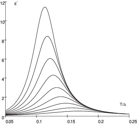
Figure 28: The dielectric susceptibility of density waves from interference of the local and the collective pinnings. The plots show the $T$ dependencies of $\epsilon^{\prime}(\omega,T)$ at various $\omega$. Calculations have been done for the formula (125) with $A/B=9$ and $U_{0}=0.5$ (both $U_{0}$ and $T$ are in units of $\Delta$). While units of $\varepsilon^{\prime}$ and $\omega$ arbitrary, their changes correspond to the experimental plots below: at each step, $\omega$ was rescaled by one order of magnitude resulting in the overall change of $\varepsilon^{\prime}$ by one order.

Figure 29: Experimental data by Nad et al [119]. Labels at the top of each curve show the frequency, in Hz.

While some features of the $T$ dependence (the rising high $T$ slope) are quite specific to CDWs and SDWs, we suggest this example as showing simultaneously a combination of several important ingredients: sensitivity of the collective pinning to elastic parameters; separation of time scales between the two types of pinning, as well as their interference in observations.

The electric polarization, being proportional to the average phase displacement $\delta\bar{\varphi}$, creates the restoring force $f_{pin}$, which may decay in time. The external electric field $\mathcal{E}$ opposes $f_{pin}$ which has two well separated contributions $f_{pin}=f_{col}+f_{loc}$. The inverse susceptibility can be defined as:

$$\varepsilon^{-1}\sim-\frac{\partial f_{pin}}{\partial\bar{\varphi}}\Rightarrow\varepsilon_{col}^{-1}+\varepsilon_{loc}^{-1}$$ (123)

Keeping track only of the major dependencies on $\omega,T,n_{i}$, we can write with the help of (112)

$$\varepsilon^{-1}=const\,n_{i}^{2}e^{-\Delta/T}+\frac{const\,\,n_{i}}{1+(i\omega\tau_{0})^{-1}\exp(-U_{\pi}/T)}$$ (124)

where the first and the second terms come from the collective and the local pinnings correspondingly. The activation law $e^{-\Delta/T}$ in the first term comes from the effect of the Coulomb hardening of the longitudinal elastic modulus which is special to quasi one-dimensional density waves.

For the model with the exponential distribution of barriers of the Sec. 11, we obtain

$$\varepsilon^{-1}=A\exp(-\frac{\Delta}{T})+B\omega^{T/U_{0}}\,,\;A\sim n_{i}^{2}\,,\,B\sim n_{i}$$ (125)

where the second coefficient $B$ is a complex weak function of $T,\omega$. In both cases, the function $\varepsilon^{\prime}(T,\omega=const)$ is not monotonic, it demonstrates a peak at $T_{max}(\omega)$ defined by the equation

$$\omega\sim{\frac{1}{\tau_{0}}}\exp(-{\frac{{E_{a}U_{0}}}{T_{max}^{2}}}+{\frac{V_{0}}{T_{max}}}\ln n_{i})$$ (126)

Numerical calculations for (125), shown on the Figure 28, are in agreement with the results of [119] shown on the Figure 29. Concerning the frequency dependence, the function $\Im\varepsilon_{DW}^{-1}(T=const,\omega)$ in (124) is monotonous, but the measured function $\Im\varepsilon_{DW}(T=const,\omega)$ shows a maximum which is also in agreement with experiments.

The interpretation of these results [29] is that different types of pinning compete to contribute to $\varepsilon^{-1}$, so that the lowest $\varepsilon$ dominates and near $T_{max}$ the pinning force is minimal. Namely, at the higher $T$ slope the $T$ dependence arises from the dispersionless (very high barriers for collective metastable states) collective pinning affected by statically screened Coulomb interactions. At the lower $T$ slope, the dispersion of $\varepsilon$ comes from the relaxation of local metastable states. With increasing $T$ at given $\omega$, the local states approach the thermal equilibrium; then $f_{loc}\rightarrow 0$, hence $\varepsilon(T,\omega)$ grows with increasing $T$ until the collective pinning force becomes dominating. Recall another, more phenomenological interpretation [119] which suggested approaching a kind of a dipole glass transition.

We conclude that the crossover picture of the local and the collective types of pinning describes altogether the susceptibility anomaly, long time relaxation and nonlinear $v-f$ characteristics. The peak of $\varepsilon(T)$ results from the competition of the local metastable plasticity with the collective pinning affected by freezing out of the Coulomb screening. In $f-v$ curves, the upper threshold field $f_{2}$ is reached when the metastable plastic deformations with shortest life time are accessed by the fast moving density wave.

14 Conclusions

In this article we have suggested an overview of the present status of our understanding of pinning phenomena in various systems, stressing the unifying aspects. Both languages of the collective and the local pinning exploit intensively the concept of metastable states.

The picture of collective pinning discussed in the first part of this review is to some extend worked out. The theory has been successfully applied already for the explanation of equilibrium phases, depinning and creep phenomena in vortex lattices, charge density waves and magnetic domain walls. The decisive step here were the understanding of thermodynamic and dynamic scaling behavior, as well as development of renormalization group methods which are capable to consider the effects of metastability emerging on large length scales even from weak pinning centers. The domain of application of this theory are large length and time scales, the critical field vicinity and the creep below it. The theoretical description of plasticity in disordered systems is still incomplete.

The picture of the local pinning, within its domain of low temperatures and not too low frequencies or velocities, can be effectively used to explain experimental data: qualitatively and even quantitatively. The advantages come from the explicit treatment of metastable states, their creation and relaxation, their relation to plasticity and topological defects. It provides also a clue to the quantum creep showing that the tunneling repulsion of crossing branches destroys the pinning.

Acknowledgments

T.N. acknowledges the hospitality of the Laboratoire de Physique Théorique et des Modèles Statistiques of the Université Paris-Sud and of the LPMMH group of the Ecole Superieure de Physique et de Chimie Industrielles de Paris were most of this work was done. He is also very grateful for the support of the Volkswagen Foundation which made this stay possible and to S.Malinin for a critical reading of the manuscript. S.B acknowledges the hospitality of the ISSP, Tokyo University and YITP, Kyoto University, the support from the INTAS grant 2212, and the assistance of N.Kirova and S.Teber.

Table 2: Frequently appearing quantities

Quantity	Symbol	see eq.,fig.,sec.
field coupling to $\mbox{\boldmath$\nabla$}u$	$\bf A$	(85)
cutoff	$a_{0}$
Burgers vector	$\bf b$	Sec.6
stiffness constant	$C=(C_{\parallel}C_{\perp}^{2})^{1/3}$	(1), (9)
elastic moduli	$C_{\parallel},\;C_{\perp}$	(9)
curvature	$\tilde{\mathcal{C}}$	(76)
dimension of the elastic object	$D$	(1)
space dimension	$d$	(2)
energy barrier on scale $L$	$E_{B}(L)$	(41)
energy of the dislocation loop of the radius $R$	$E_{DL}(R)$	(113)
soliton energy	$E_{s}$	Figure19, Sec.7.2.2,
energy difference between low lying states	$\Delta E$	(21)
frequency dependent barrier	$E_{\omega}$	(48)
energy branches (1: stable, 2: metastable, +: accending, -: descending)	$E_{1,2}$, $E_{\pm}$	(95,96)
free energy	$\mathcal{F}(L,u)$	(127)
disorder dependent free energy	$\mathcal{F}_{R}$	(18)
forces from the single impurity $F_{a}$, $a=+,-,1,2$	$F_{\pm}(\theta)=E_{\pm}^{\prime}$	(97)
driving force density	$f$	(42), (60)
pinning threshold	$f_{c}\approx f_{p}=Cl/L_{p}^{2}$	(66), (69)
pinning forces: total, collective, local and its maximum	$f_{pin}$, $f_{col}$, $f_{loc}$, $f_{max}$	Fig.23, Sec.13.2
temperature dependent force	$f_{T}$	(46)
frequency dependent characteristic force	$f_{\omega}$	(49)
free enthalpy	$G$	(88)
random pinning force	$g({\bf x},u)$	(60)
variational energy	$H=W(\psi)+V(\psi-\theta)$	(94)
Hamiltonian	$\cal H$	(1)
tunneling rate	$I_{\omega}$	(117)
dynamic parameters	$K_{\omega}$	(118)
length scale (variable)	$L$	(15)
system size	$L_{0}$
scale on which tilted potential vanishes	$L_{f}$	(42)
Larkin length	$L_{p}$	(16)
frequency dependent scale	$L_{\omega}$	(48)
frequency dependent diffusion length	$\tilde{L}_{\omega}$	(82)
correlation length of the random potential	$l$	(15)
soliton length	$l_{s}$	Figure21, Sec.7.2.2
concentration of impurities	$n_{imp},n_{i}$	(4)
occupation numbers of terms $\pm$, there difference and its equilibrium value	$n_{\pm}$, $n=n_{+}-n_{-}$, $n_{eq}$	(103,104)
probability distribution of excited states	$P(\Delta E,L)$	(21)
distribution functions for $U$ and $\tau$	$P_{U}$, $P_{\tau}$	(120)
wave vector of charge density wave	$\bf Q$	(7)
disorder average	$\langle...\rangle_{R}$	(5)
correlator of the random potential	$R$	(6), (10)
correlation function of the random potential	$R(u)$	(6)
running effective $t/\tau$	$s(\theta(t))$	(141)
thermal average	$\langle...\rangle_{T}$	(17)
temperature	$T$	(19)
energy scale due to pinning	$T_{p}=Cl^{2}L_{p}^{D-2}$	(18)
position vector (D-dimensional)	$\bf x$	(1)
barrier branch $E_{3}$ and metastable sate decay activation $U$	$U(\theta)=E_{3}-E_{2}$, $U_{\pi}=U(\pi)$	(96,98)
displacement field (N-dimensional)	$u$	(1)
pinning potential, its magnitude and threshold values	$V(\varphi)$; $V$, $V_{1}$,$V_{2}$	(102),C
random potential	$V_{R}({\bf x},u)$	(1), (2)
velocity	$v$	(44)
phase velocity	$v=-d\bar{\varphi}/dt$	Tab.1, App.D.1
impurity potential	$v_{R}(\mathbf{x},\mathbf{z})$	(2), (4)
strength of individual pinning center $i$	$V_{i}$	(4)
deformation energy	$W(\psi)$	(94)
roughness	$w_{R}(L)$	(15)
dynamical critical exponent	$z$	(25)
exponents at the $T=0$ depinning transition	$\tilde{\alpha},\tilde{\beta},\tilde{\zeta},\tilde{z},\tilde{\nu}$	(72)-(75)
mobility	$\gamma$	(39)
correlator of random pinning forces	$\Delta(u)$	(62)
$\delta$-function of width $l$	$\delta_{l}({\bf x})$	(3)
quantum splitting of branches	$\delta_{q}=\hbar/\tau_{q}$	116
roughness exponent	$\zeta$	(25)
thermal noise	$\eta({\bf x},t)$	(39)
pinning phase mismatch and its special values	$\theta=\theta_{i}(t)=\bf\textbf{}{Qx}_{i}-\bar{\varphi}(t)$; $\theta_{e}$, $\tilde{\theta}_{e}$, $\theta_{m}$, $\theta_{e}^{\ast}$	(92), Figs.17,19
barrier exponent	$\mu=\chi/(2-\zeta)$	(43)
size distribution of excited states	$\nu(L)$	(23)
correlation length	$\xi$	(73)
relaxation time	$\tau=\tau_{0}\exp[U/T]$	(104)
scaling function	$\Phi(y)$	(80)
phase field of the charge density wave	$\varphi({\bf x},t)$	(8)
mean value of phase	$\bar{\varphi}(t)$	(92)
soliton profile	$\varphi_{s}(x-X)$	Figs.21,16
exponent describing the free energy fluctuations	$\chi$	(18)
response function and the susceptibility of CDWs	$\chi\sim\varepsilon$	(123)
local phase mismatch and its special values	$\psi=\varphi(\bf{x}_{i},t)-\bar{\varphi}(t)$, $\psi_{e}$, $\psi_{e}^{\ast}$	(92,99)
frequency	$\omega$	(47)
pinning frequency	$\omega_{p}=\gamma C/L_{p}^{2}=Cf_{p}/l=v_{p}/l$	(48)

APPENDICES.

Appendix A Free energy fluctuations in $D=1$ dimensions

An illustrative example is given by a linear $D=1$-dimensional object such as a magnetic flux line with the boundary conditions $u(L)\equiv u$ and $u(0)=0$. Changing $u$ enforces the object to see another disorder environment. Using the transfer matrix technique, it can be shown that $F(L,u)$ obeys the equation [45]

$$\frac{\partial\mathcal{F}_{R}}{\partial L}=\frac{T}{2C}\frac{\partial^{2}\mathcal{F}_{R}}{\partial u^{2}}-\frac{1}{C}\left(\frac{\partial\mathcal{F}_{R}}{\partial u}\right)^{2}+V_{R}(L,u).$$ (127)

As a side remark we mention that if we read $L$, $u$ and $\mathcal{F}_{R}$ as time, space and height coordinates, respectively, eq. (127) becomes the Kardar-Parisi-Zhang-equation, which describes the height profile of a growing surface under the random influx $V_{R}(L,u)$ of particles [123]. The correlations of the restricted free energy show the following scaling behavior:

$$\left\langle\big{(}\mathcal{F}_{R}(L,u)-\mathcal{F}_{R}(L,u^{\prime})\big{)}^{2}\right\rangle_{R}^{1/2}=T_{p}\left(\frac{L}{L_{p}}\right)^{\chi}\Phi\left(\frac{u-u^{\prime}}{w_{R}(L)}\right),$$ (128)

For small values of the argument $y=({u-u^{\prime}})/{w_{R}(L)}$ of $\Phi$ the difference of the free energies should not depend on $L$ since the configurations dominating the free energy will be the same for most parts of the elastic object (apart from $x$ close to $L$). This gives $\Phi(y)\sim y^{\chi/\zeta}$. For large arguments $y$ the elastic stiffness dominates over the disorder and $\left\langle\big{(}\mathcal{F}_{R}(L,u)-\mathcal{F}_{R}(L,u^{\prime})\big{)}^{2}\right\rangle_{R}^{1/2}\sim\frac{|u^{2}-{u^{\prime}}^{2}|}{L}$ as in pure systems. A numerical solution of (127) shows that for large $L$ and intermediate values of $y$ the free energy $\mathcal{F}_{R}(L,u)$ forms a rugged landscape as a function of $u$ with typical valleys of width $w(L)$ separated by hills of height $T_{p}(L/L_{p})^{\chi}$ [124]. The general picture of a rugged energy landscape as concluded from eq. (128) is believed to hold also for higher dimensional elastic objects.

Appendix B Strong pinning in $D=1$–dimensional CDWs

To give a specific example for the case of strong pinning, we consider a lattice model for a charge density wave with the Hamiltonian given by

$$H=\sum_{<i,j>}\frac{1}{2}C_{i,j}(u_{i}-u_{j})^{2}-\sum_{i}V_{i}\cos\left(2\pi(u_{i}-\kappa_{i}))\right)$$ (129)

where $2\pi\kappa_{i}=-{\bf Qx}_{i}$ and ${\bf x}_{i}$ is a random impurity positions at which $V_{i}\neq 0$. If we assume for simplicity $V_{i}\equiv V$ for all $i$ and consider the limit $V\rightarrow\infty$, then $u_{i}=\kappa_{i}+n_{i}$ with $n_{i}$ integer and the Hamiltonian can be rewritten as

$$H=\sum_{<i,j>}\frac{1}{2}C_{i,j}(n_{i}-n_{j}+\kappa_{i}-\kappa_{j})^{2}$$ (130)

The minimization of this Hamiltonian leads to a set of integers $\{n_{i,0}\}$ from which a well defined result for ground state and hence the roughness $w_{R}$ follows. The ground state consists of regions of constant $n_{i}$ separated by oriented domain walls at which $n_{i}$ changes by $\pm 1$. A very simple situation exists in $d=1$ dimensions, where $<i,j>=i,i+1$ and the ground state follows trivially as $n_{i+1}=n_{i}+[\kappa_{i+1}-\kappa_{i}]$. Here $[...]$ denotes the Gauss bracket which replaces its argument by the closest integer. Thus the $u_{i}$ undergo a random walk and hence $\zeta=1/2$. For a more detailed discussion of the one-dimensional case see e.g. [125].

The specific Transfer Matrix technics (Appendix A) in the dimension $D=1$ allows for a more detailed description of interference between the pinning and the thermal motion [53]. Thus for temperatures high in compare to the characteristic elastic energy $T\gg T^{\ast}\sim Cn_{imp}$, and arbitrary with respect to $V$, the heat capacitance $c(T)$ is

$$c\approx n_{imp}/2~{},~{}T\ll V\ \ ;\ \ c\sim n_{imp}(V/T)^{2}~{},~{}T\gg V\$$

In the same regime, the correlations of the order parameter $\cos(2\pi u_{i})$ decay exponentially with the correlation length $\xi(T)$ such that $\xi^{-1}=\xi_{T}^{-1}+\xi_{R}^{-1}$. Here $\xi_{T}\sim C/T$ is the correlation length of a pure system while the randomness contribution to $\xi^{-1}$ is

$$\xi_{R}\sim n_{imp}^{-1}\left(I_{0}(V/T)/I_{1}(V/T)\right)^{2}$$

where $I_{m}$ are the modified Bessel functions.

For low temperatures with a constraint to the strong pinning regime $T\ll T^{\ast}\ll V$ the correlation function of displacements behaves as a kind of the Mott law

$$\left\langle\left\langle\left|u_{i}-u_{j}\right|\right\rangle_{T}\right\rangle_{R}\sim\left|i-j\right|n_{imp}\left(\frac{T^{\ast}}{T}\right)^{1/4}\exp\left(-cnst\left(\frac{T^{\ast}}{T}\right)^{1/4}\right)$$

This nontrivial $T$ dependence appears because thermal jumps take place primarily within segments of an optimal spacing $\left|i-j\right|_{opt}\sim n_{imp}^{-1}(T^{\ast}/T)^{1/2}$ which is much larger than the typical one $n_{imp}^{-1}$.

Appendix C Details on metastable branches.

Here we give details to the results of Sec. 7 on the energy branches and their special points in the language of the CDWs and its phase.

Consider first the termination points defined in (99); all quantities at this point will be labelled by the index $e$. Expanding at the vicinity of the end point

$$\psi=\psi_{e}+\delta\psi;\quad\theta=\theta_{e}+\delta\theta,\quad\delta\theta<0$$ (131)

we find from (95), (99) and (98) the solutions

$$\delta\psi_{3,2}=\pm\left({2{\frac{V_{e}^{\prime\prime}}{H_{e}^{\prime\prime}}}|\delta\theta|}\right)^{1/2}\,,\;U=V_{e}|\delta\theta|^{3/2}\,,\;V_{e}=-{\frac{2}{3}}{\frac{(2V_{e}^{\prime\prime})^{3/2}}{(H_{e}^{\prime\prime})^{1/2}}\,,\;}H_{e}^{\prime\prime}=V_{e}^{\prime\prime}+W_{e}^{\prime\prime}$$ (132)

As a function of $V$, the coefficient $V_{e}$ is singular at $V=V_{1}$ when the end point emerges and at $V=V_{2}$ when it annihilates with the next one, $\theta\rightleftharpoons\tilde{\theta}_{e}$:

1. Consider the emergence of metastable branches when the points $\theta_{e},-\theta_{e}+2\pi$ split from the point $\pi$. We find

$$V=V_{1}+\delta V\geq V_{1}\ :\;\theta_{e}-\pi\sim(\delta V)^{3/2}\,,\;U\sim(\delta V)^{-1/4}(-\delta\theta)^{3/2}\,,\;F_{e}\sim(\delta V)^{1/2}\qquad$$ (133)

2. Consider the crossover to the unrestricted bistability: $V\rightarrow V_{2}$ when the two sets of end points $\theta_{e},\tilde{\theta}_{e}$ join together and with the point $\theta_{m}$ of the minimal barrier. At $V=V_{2}+\delta V$ $<V_{2}$ the degeneracy is lifted and the branch crossing point $(\theta_{m},\psi_{m})$ splits into two end points

$$\theta_{e},\,\tilde{\theta}_{e}=\theta_{m}\mp\delta\theta_{e}\;\;\delta\theta_{e}\sim\sqrt{-\delta V}\,;\;U\sim(\delta V)^{3/4}(-\delta\theta)^{3/2}$$ (134)

At $V>V_{2}$, $U(\theta)$ passes through the minimum $U_{min}\sim(\delta V)^{3/2}$ at $\theta=\theta_{m}$. For both signs of $\delta V$ we can write an interpolation

$$V\lessgtr V_{2}:\;U=\left(B_{1}\delta\theta^{2}+B_{2}\right)^{3/2}\,\,;\;B_{1}\sim\delta V^{1/2}\,,\;\ B_{2}\sim\delta V$$

3. Consider the limit of very strong impurities which allows for an explicit treatment. The equation $W^{\prime}(\psi)+V\sin(\psi-\theta)=0$ at $V\gg\max W^{\prime}$ has the following solutions:

$$E_{+} : \psi\approx\theta-V^{-1}W^{\prime}(\theta)\,,\;E_{+}\approx W(\theta)-(2V)^{-1}W^{\prime 2}(\theta)$$

$$E_{-} : \psi\approx\theta-2\pi-V^{-1}W^{\prime}(\theta-2\pi)\,,\;E_{-}\approx W(\theta-2\pi)-(2V)^{-1}W^{\prime 2}(\theta-2\pi)$$

$$E_{3} : \psi\approx\theta-\pi+V^{-1}W^{\prime}(\theta-\pi)\,,\;E_{3}\approx 2V+W(\theta-\pi)-V^{-1}W^{\prime 2}(\theta)$$

$$U = E_{3}-E_{+}\approx 2V+W(\theta-\pi)-W(\theta)\,,\;W^{\prime}(\theta_{m}-\pi)=W(\theta_{m})$$

4. Fortunately, for a point impurity we can order the branches and simplify the energy a priori even at arbitrary $V$. In what follows, $\pi<\theta<2\pi$, while $W,W^{\prime}$ are functions of $\psi$ at $-2\pi<\psi<2\pi$. For each term, we determine its own function $\psi=\psi_{a}(\theta)$ with $a=\{-,+,3\}\equiv\{1,2,3\}$ (within the selected semiperiod of $\theta$).

$$\psi = \psi_{+}:\theta=\psi+\arcsin\frac{W^{\prime}}{V}\,,\;E_{+}=W-V\sqrt{1-\frac{W^{\prime 2}}{V^{2}}}\,+V$$

$$\psi = \psi_{-}:\theta=\psi+\arcsin\frac{W^{\prime}}{V}+2\pi\,,\;E_{-}=W-V\sqrt{1-\frac{W^{\prime 2}}{V^{2}}+V}$$

$$\psi = \psi_{3}:\theta=\pi+\psi-\arcsin\frac{W^{\prime}}{V}\,,\;E_{3}=W+V\sqrt{1-\frac{W^{\prime 2}}{V^{2}}}+V$$

$$U(\theta) = E_{b}(\psi_{b}(\theta))-E_{+}(\psi_{+}(\theta))\,$$

These expressions were the bases for our plots on Figures 18,22.

5. Consider in more details the overshooting branches which appear due to special long range effects of dislocations (recall the end of the Section 7.2 and the Section 9.1). This is the regime of small $\delta\psi\approx\psi-2\pi$ and $\delta\theta=\theta-2\pi$. Here, $V$ is close to its minimum $\delta V\approx b/2(\delta\psi-\delta\theta)^{2}$, $b=V^{\prime\prime}(0)$; $W$ is close to its maximum $W_{2\pi}=2E_{s}$, but the expansion is not analytical. We shall write it, according to (113) taken for $d=3$, as $\delta W=-4/3a(-\delta\psi)^{3/2}$ where $a\sim CR$ for the dislocation loop of the radius $R$. The minimization of $H$ over $\psi$ gives $\delta\theta=\delta\psi+2a/b(-\delta\psi)^{1/2}=0$.

At $\delta\theta<0$, there is one solution $\delta\psi=-\left(a/b+((a/b)^{2}-\delta\theta)^{1/2}\right)^{2}$; it gives the branch $E_{+}$ approaching the end of the period, $\theta\rightarrow 2\pi-0$ with some deficiency $E_{+}(2\pi)<0$: $\delta E_{+}=-(8/3)a^{4}/b^{3}$ corresponding to the retardation $\delta\psi=-(2a/b)^{2}$.

At $\delta\theta>0$, there are two solutions $\delta\psi=-\left(a/b\pm((a/b)^{2}-\delta\theta)^{1/2}\right)^{2}$. Here the sign $-$ corresponds to the barrier branch $E_{3}^{*}$, the sign $+$ corresponds to the overshooting part $E_{+}^{*}$ of the branch $E_{+}$.

Entering the next circle $\delta\theta>0$, the energy $E_{+}$ keeps increasing, passing through the energy $2E_{s}$ at $\delta\psi=-\left(3a/2b\right)^{2}\,,\,\delta\theta=3/4(a/b)^{2}$. Further on it crosses with the branch $\tilde{E}_{+}$ to become metastable. Since then, the difference $E_{3}^{*}-E_{+}^{*}=U$ gives the relaxation barrier. Finally, the two solutions $E_{+}$ and $E_{3}$ collapse at the termination point

$$\delta\theta_{e}=(a/b)^{2}\,,\;\,\delta\psi_{e}=-(a/b)^{2},\;\delta H_{e}=20a^{4}/3b^{3}$$

The above results give rise to the picture of the Figure 24 and related conclusions.

Appendix D Details on the kinetic equation.

The kinetic equation is derived from the balance law for occupation numbers of branches $+,-$, see Eq. (103):

$${\frac{dn_{+}}{dt}}=W_{\mp}n_{+}+W_{\pm}n_{-}\ ,\quad{\frac{dn_{-}}{dt}}=W_{\pm}n_{-}+W_{\pm}n_{+}$$ (135)

Here $W_{\pm},W_{\pm}$ are transition rates between the branches and the full time derivative is

$${\frac{d}{dt}}={\frac{\partial}{\partial t}}+\dot{\theta}{\frac{\partial}{\partial\theta}};\quad\dot{\theta}={\frac{d\theta(t)}{dt}=v}$$ (136)

$$W_{\mp}/W_{\pm}=\exp{(\Delta E/T)\,},\quad W_{\pm},\ W_{\mp}\sim\exp{(-E_{b}/T)},\quad\Delta E=E_{+}-E_{-}$$ (137)

The relaxation rate is

$${\frac{1}{\tau(\theta)}}=W_{\pm}+W_{\mp}\sim{\frac{1}{\tau_{0}}}\cosh{\frac{\Delta E}{2T}}\exp\left(\frac{E_{+}+E_{-}-2E_{3}}{2T}\right)$$ (138)

where $\tau_{0}^{-1}$ is an attempt rate. For $\Delta E>>T$, $\quad\tau\sim\exp(U/T)$ with the activation energy $U=E_{3}-E_{2}$. Notice that at the end points the metastable branch disappears and there must be $\tau(\theta\rightarrow\theta_{e})\rightarrow 0$. Still the expression (104) leaves us with small but finite value of $\tau\sim\tau_{0}$ even at $U(\theta_{e})\rightarrow 0$. Hence it should be corrected to provide $\tau\rightarrow 0$ at $U\ll T$; it happens via a dependence $\tau_{0}(\theta)$ which plausible form is $\tau_{0}\sim(\theta-\theta_{e})^{k},\ k>1$.

D.1 Stationary motion.

Consider a stationary process when the density wave moves at a constant phase velocity $v=-\dot{\bar{\varphi}}=\dot{\theta}=const$, then $\partial n/\partial t=0$. Now the solution of the Eq. (104) is trivial, but the boundary conditions must be properly specified. Suppose first that there are no end points which is the case of very strong impurities $V>V_{2}$, see the Figure 19. Then for $\theta$ approaching $2\pi$, both branches $+$ and $-$ contribute to initial conditions for the branch $+$ at $\theta=0$ adding the pair of solitons at infinity, see the Figure 16. Contrarily, there is no source for the branch $-$ at $\theta=0$. This conditions read

$$\left.{\frac{\partial n_{+}}{\partial\theta}}\right|_{0}={\frac{\partial}{\partial\theta}}(n_{+}+n_{-})_{2\pi}=0\,,\;\mathrm{hence}\quad n(0)=n_{eq}$$ (139)

The solution of (104), (139) is

$$n=n_{eq}(s_{0})e^{s_{0}-s}+\int_{s_{0}}^{s}n_{eq}(s_{1})e^{s_{1}-s}ds_{1}$$ (140)

where $s(\theta)$ is an effective $t/\tau$ over the branch:

$$s=s(\theta)=\int_{\pi}^{\theta}{\frac{d\theta}{v\tau(\theta_{1})}};\quad s_{0}=s(0)=-s(2\pi)$$ (141)

(We shall keep the same notations for functions of $\theta$ and of $s=s(\theta)$.) At presence of end points ( right $\theta_{e}$ and left $2\pi-\theta_{e}$) there is only one branch of lowest energy $E_{1}$ which survives beyond $(2\pi-\theta_{e},\ \theta_{e})$, that is

$$0<\theta<2\pi-\theta_{e}\ :\quad n=1\,;\;\theta_{e}\leq\theta<2\pi\ :\quad n=-1$$ (142)

The contributions of these monostable regions to the pinning force are exactly compensated as it should be. Within the bistability region $(2\pi-\theta_{e},\ \theta_{e})$ the solution is

$$n=\int_{0}^{\infty}{n_{eq}(s-s_{2})\exp(-s_{2})ds_{2}}$$ (143)

The substitution to the general expression for the force (105) yields (at presence of end points)

$$f=n_{i}\int_{-\infty}^{\infty}{ds\Delta E}\int_{0}^{\infty}{ds_{2}e^{-s_{2}}\left[n_{0}(s-s_{2})-n_{0}(s)\right]}$$ (144)

Mostly we shall consider the case of low $T$ when $\Delta E\gg T$ in essential regions, then

$$n_{eq}(s)\approx-\mathrm{sgn}s,\quad n-n_{eq}=\Theta(s)e^{-s}$$ (145)

($\Theta$ is the unit step function). The point of symmetrical population, $n=0$, is shifted to $\ s=\ln 2$. At $0<s\leq\ln 2$ there is an inverted population, $n_{2}>n_{1}$ as shown on the Fig. 17. Finally the expression (144) is simplified to the form (106).

D.2 Various regimes for $f(v)$.

Small velocities for all cases.

At $v\tau_{\pi}\ll 1$, $s(\theta)$ is large almost everywhere, except for a vicinity of $\pi$ where the barrier activation energy takes its largest value $U(\pi)=U_{\pi}$; then we should use (144). Namely, if for largest $\tau(\pi)=\tau_{\pi}$ we have $v\tau_{\pi}\ll 1$, then $s\sim 1$ already at $\theta-\pi\sim v\tau_{\pi}\ll 1$ so that at $(\theta-\pi)\sim 1$ we have $s\gg 1$, then the series in $v$ is well convergent. In lowest order of $v\tau$ we find

$$f\approx\pi n_{i}\int_{0}^{\infty}ds\Delta E{\frac{d^{2}n_{eq}}{ds^{2}}}=\pi n_{i}\int{\frac{v\tau/T}{\cosh^{2}(\Delta E/2T)}}\left({\frac{d\Delta E}{d\theta}}\right)^{2}d\theta\approx v\tau_{\pi}F_{\pi}$$ (146)

At low $T$ the dependence of the expression under the last integral in (146) is governed by the factor, see (138), $\exp\left[-\left((E_{3}-E_{2})-(E_{2}-E_{1})\right)/T\right]$. It has a maximum $\exp(-U_{\pi}/T))$ at $\theta=\pi$ and we arrive at the result (108).

At higher velocities, still only the vicinities of the crossing point $\theta\approx\pi$ is important, but we must take into account the reduction of the barrier with increasing $\theta$: $U=U_{\pi}-F_{\pi}(\theta-\pi)/2\pi$. We obtain

$$f=n_{i}T\int\frac{ds\exp(-s)}{s+v\tau_{\pi}F_{\pi}/(2\pi T)}\approx\left\{\begin{array}[]{cc}n_{i}\tau_{\pi}F_{\pi}v&\mathrm{at\;}v\tau_{\pi}F_{\pi}T\ll 1\\ n_{i}T\ln(v\tau_{\pi}F_{\pi}/T)&\mathrm{at}\;v\tau_{\pi}F_{\pi}/T\gg 1\end{array}\right.$$ (147)

High velocities: restricted metastability. Let $v\tau_{\pi}>>1$, then $s\sim 1$ only at $\theta\approx\theta_{e}$. The form (107) is more appropriate for calculations. Since $e^{-s}-1$ is small at $s\ll 1$ i.e. at almost all $\theta$, then only a vicinity of $\theta_{e}$ contribute, hence we can take $F=F_{e}$ at $\theta=\theta_{e}$. We obtain

$$f=f_{max}-2\pi n_{i}F_{e}\int_{\pi}^{\theta_{e}}d\theta\left(1-e^{-s(\theta)}\right)\,\,;\;f_{max}=2\pi n_{i}\Delta E_{e}$$ (148)

Remind that at $\theta_{e}$ the activation $U=E_{3}-E_{2}\rightarrow 0$ vanishes while the force is finite $F_{e}=\partial\Delta E/\partial\theta\neq 0$. We find

$${f_{max}-f}\sim F_{e}n_{i}\delta\theta_{v}$$

where $\delta\theta_{v}$ is defined by the condition

$$s(\delta\theta_{v})\sim\frac{v_{e}}{v}\delta\theta_{v}^{-\nu+1}{\exp(-\frac{V_{e}}{T}\delta\theta_{v}^{\nu})}\sim{1};\quad v_{e}=\left(\frac{T}{V_{e}}\right)^{1/\nu}{\frac{1}{\tau_{0}}}$$ (149)

and we arrive at the result (110), valid in this simple form at $v_{e}\exp(-V_{e}/T)\ll v\ll v_{e}$.

High velocities: unrestricted metastability.

The calculations are similar to the above case of the restricted metastability and we shall skip equivalent steps. The difference is that now there is a high velocity range $v\gg v_{m}=\max\tau^{-1}$ where the $1/v$ expansion is valid:

$$f=2n_{i}\left\{\Delta E(2\pi)-\frac{2}{v}\int_{\pi}^{2\pi}{{\frac{d\theta}{\tau(\theta)}(}\Delta E(2\pi)-\Delta E(\theta))}\right\}$$ (150)

D.3 Linear response.

Consider $\dot{\theta}$ as a perturbation in the kinetic equation and expand as $n=n_{eq}(\theta)+\delta n(\theta,t)$:

$$\left({\frac{\partial}{\partial t}+\frac{1}{\tau}}\right){\delta n}+\dot{\theta}\frac{\partial}{\partial\theta}n_{eq}=0\,;\;f=n_{i}\int_{\pi}^{\theta_{max}}{d\theta F(\theta)\delta n(\theta)}$$ (151)

In the Fourier representation we have

$${\delta n}_{\omega}=\frac{i\omega\theta_{\omega}}{\left(-i\omega{+\tau}^{-1}\right)}\frac{d}{d\theta}{n}_{eq}$$ (152)

$$f_{\omega}=\frac{\theta_{\omega}n_{i}}{\left(-1{+(i\omega\tau)}^{-1}\right)}\int_{\pi}^{\theta_{e}}{d\theta{\frac{d\Delta E}{d\theta}\frac{d}{d\theta}{n}_{eq}}}\approx\frac{F_{\pi}\theta_{\omega}n_{i}}{\left(-1{+(i\omega\tau)}^{-1}\right)}$$ (153)

$$\chi_{\omega}^{-1}=\frac{\delta f_{\omega}}{\delta\theta_{\omega}}=\frac{n_{i}F_{\pi}}{1+1/i\omega\tau},$$ (154)

which confirms (112).

References

- [1] Monceau, P., 1985, in ”Electronic properties of quasi one-dimensional compounds.”, P. Monceau ed., Reidel Publ. Co.
- [2] Grüner, G. 1994, ”Density Waves in Solids”, Addison-Wesley Publ. Company, Reading.
- [3] Gor’kov, L., and Grüner, G., 1989, ”Charge Density Waves in Solids”, Elsevier Sci. Publ., Amsterdam, 6, 365.
- [4] Dumas, J., and Schlenker, C., 1993, Int. Journ. Mod. Phys. B 7, 4045.
- [5] Proceedings of the International Workshop on Electronic Crystals, June 1993, ed. by Brazovskii, S., Monceau, P.,1993, J. Phys. France IV, Colloque C2 3.
- [6] Proceedings of the International Workshop on Electronic Crystals, 1999, ed. by Brazovskii, S., Monceau, P., 1999, J. Phys. France IV, 9.
- [7] Proceedings of the International Workshop on Electronic Crystals, September 2002, ed. by Brazovskii, S., Kirova, N., and Monceau, P., 2002, J. Phys. France IV, 12.
- [8] X. Zhu, P. B. Littlewood, and A. J. Millis, 1994, Phys. Rev. B 50, 4600; and rfs. theirin.
- [9] Giamarchi, T., and Orignac, E., in New Theoretical Approaches to Strongly Correlated Systems, ed. by A.M. Tsvelik, Kluwer 2001.
- [10] Blatter, G., Feigel’man, M. V., Geshkenbein, V. B., Larkin, A. I. and Vinokur, V. M., 1994, Rev. Mod. Phys., 66, 1125.
- [11] Nattermann, T., and Scheidl, S., 2000,Adv. in Physics, 49, 607-704.
- [12] Lyuksyutov, I., Naumovets, V. and Pokrovsky, V., 1992, Two-dimensional Crystals, Academic Press, Boston.
- [13] see, e.g., Young, P.A., (ed.), 1999, Spin Glasses and Random Fields, World Scientific, Singapoore.
- [14] Fisher, D.S., 1998, Phys. Rep. 301, 113.
- [15] Kardar, M., 1998, Phys. Rep. 301, 85.
- [16] Haasen, H.P., 1958, in Berichte der Göttinger Akademie der Wissenschaften.
- [17] Larkin, A.I., 1970, Sov. Phys. JETP 31, 784.
- [18] Larkin, A.I., and Ovchinnikov, Yu.N., 1979, J. Low Temp. Phys. 34, 409.
- [19] Fukuyama, H., 1976, J. Phys. Soc. Jpn. 41, 513, 542.
- [20] Fukuyama, H., and Lee, P.A., 1978, Phys. Rev. B 17, 535.
- [21] Lee, P.A., and Rice, T.M., 1979, Phys. Rev. B 19, 3970.
- [22] Nattermann, T., 1990, Phys. Rev. Lett. 64, 2454.
- [23] Korshunov, S.E., 1993, Phys. Rev. B 48, 3969.
- [24] Giamarchi, T., and Le Doussal, P., 1994, Phys. Rev. Lett. 72, 1530; 1995, Phys. Rev. B 52, 1242.
- [25] Fisher, D.S., 1985, Phys. Rev. B 31, 7233.
- [26] Fisher, D.S., 1986, Phys. Rev. Lett. 56, 1964.
- [27] Caroli, C., in [7], p. 269, and rfs. therein.
- [28] Larkin, A.I., 1994, Sov. Phys. JETP 105, 1793.
- [29] Larkin, A.I., and Brazovskii, S., 1995, Sol. State Commun. 93, 275.
- [30] Brazovskii, S., in [113], p.467.
- [31] Brazovskii, S., and Larkin, A.I., in [6] and cond-mat/9911100.
- [32] Nattermann, T., 2000, in Spin Glasses and Random Fields, ed. by Young, A.P., World Scientific, Singapoore.
- [33] Nattermann, T., 1985, Z. Physik, B54,247 (1984), Phys. stat. sol. (B), 132, 125.
- [34] Emig, T., and Nattermann, T., 1998, Phys. Rev. Lett. 81, 1469.
- [35] Grinstein, G., and Ma, S.-K., 1982, Phys. Rev. Lett. 49, 685.
- [36] Landau, L.D., and Lifshitz, L.F., 1989, Theoretical Physics, Vol. 7, Akademie-Verlag Berlin.
- [37] Efetov, K.B., and Larkin, A.I., 1977, Sov. Phys. JETP. 45, 1236.
- [38] Andrei, E.Y., et al., 1988, Phys. Rev. Letters 60, 2765.
- [39] Willet, R.L., et al., 1989, Phys. Rev. B 38, R 7881.
- [40] Giamarchi, T., 2002, in Proceedings of the NATO ASI “Field Theory of Strongly Correlated Fermions and Bosons in Low-Dimensional Disordered Systems”, Kluwer.
- [41] Imry, Y. and Ma, S.K., 1975, Phys. Rev. Lett. 35, 1399.
- [42] Alava, M.J., et al., 2001, in “Phase Transitions and Critical Phenomena”, ed. by C. Domb and J.L. Lebowitz, Vol. 18, p.145, Academic Press.
- [43] Villain, J., and Semeria, B., 1983, J. Phys. (Paris), 44, L 889.
- [44] Villain, J., and Fernandez, J.F., 1984, Z. Physik B 54, 139.
- [45] Huse, D.A., Henley, C.L., and Fisher, D.S., 1985, Phys. Rev. Lett. 55, 2924.
- [46] Nattermann, T., 1987, Europhysics Lett. 4, 1241; Nattermann, T., 1988, Phys. Rev. Lett 60, 2701.
- [47] Mezard, M., 1990, J. Phys. (Paris) 51, 1831.
- [48] Fisher, D.S., and Huse, D.A., 1991, Phys. Rev. B43, 10728.
- [49] Schulz, U., Villain, J., Brézin, E., and Orland, H. 1988, J. Stat. Phys., 51, 1.
- [50] Korshunov, S.E., 2001, Phys. Rev. B 63, 174514.
- [51] Anderson, P.W., Halperin, B.I., and Varma, C.M., 1972, Phil. Mag. 8 (25), 1.
- [52] Schehr, G., Giamarchi, T., and Le Doussal, P., 2003, Phys. Rev. Lett. 91, 117002.
- [53] Brazovskii, S., 1979, Sov. Phys.: JETP 49, 504.
- [54] Patashinsky, A.Z. and Pokrovsky, V., 1979, “Fluctuation Theory of Phase Transitions”, Pergamon Press Oxford.
- [55] Amit, D.J., 1984, “Field Theory, the Renormalization Group, and Critical Phenomena”, World Scientific Singapore.
- [56] Balents, L. and Fisher, D.S., 1993, Phys. Rev. B 48, 5949.
- [57] Balents, L., Bouchaud, J.P., and Mezard, M., 1996, J. Phys. I (Paris) 6 1007.
- [58] Chauve, P., Le Doussal, P., and Wiese, J.-K., 2001, Phys. Rev. Lett. 86, 1785.
- [59] Lässig, M., 1998, Phys. Rev. Lett. 80, 889.
- [60] For a review see also Halpin-Healy, T., and Zhang, Y.C., 1995, Physics Reports 254, 215.
- [61] Emig, T., Bogner, S., and Nattermann, T., 1999, Phys. Rev. Lett. 83, 400; S. Bogner, T. Emig and T. Nattermann, 2001, Phys. Rev. B 63 , 174501.
- [62] Kierfeld, J., Hwa, T., and Nattermann, T., 1997, Phys. Rev. B. 55, 626.
- [63] Carpentier, D., Le Doussal, P., and Giamarchi, T., 1996, Europhys. Lett. 35, 15193.
- [64] Fisher, D.S., 1997, Phys. Rev. Lett. 78, 1964.
- [65] Kierfeld, J., 1998, Physica C 300, 171.
- [66] Kierfeld, J., and Vinokur, V., 2000, Phys. Rev. B 61, R14928.
- [67] Feigel’man, M., 1980, Sov. Phys. 52, 555.
- [68] Glatz, A., and Nattermann, T., 2002, Rev. Lett.88, 256401.
- [69] Littlewood, P.B., and Rammal, R., 1988, Phys. Rev. B 38, 2675; Myers, C.R., and Sethna, J.P., 1993, Phys. Rev. B 47, 11194.
- [70] Drossel, B., and Kardar, M., 1995, Phys. Rev. E, 52, 4841.
- [71] Mikheev, L.V., Drossel, B., and Kardar, M., 1995, Phys. Rev. Lett., 75, 1170.
- [72] Ioffe, L. B., and Vinokur, V. M.,1987, J. Phys. C 20, 6149.
- [73] Nattermann, T., 1987, Europhys. Lett., 4, 1241.
- [74] Radzihovsky, L., 1998, Talk E37 8 given at the March Meeting of the American Physical Society.
- [75] Chauve, P., Giamarchi, T., and Le Doussal, P., 1998, Europhys. Lett. 44, 110.
- [76] Narayan, O., and Fisher, D.S., 1992, Phys. Rev. Lett., 68, 3615; Phys. Rev. B, 46, 11520.
- [77] Nattermann, T., Stepanow, S., Tang, L.-H., and Leschhorn, H., 1992, J. Phys. II France 2, 565 (1483); 1997, Ann. Phys. (Leipzig) 6, 1.
- [78] Narayan, O., and Fisher, D.S., 1993, Phys. Rev. B 48, 7030.
- [79] Ertas, D., and Kardar, M., 1994, Phys. Rev. E 49, R2532.
- [80] Vinokur, V.M., and Nattermann, T., 1997, Phys. Rev. Lett. 79, 3471.
- [81] Glatz, A., and Nattermann, T., 2003, cond-mat/0304050.
- [82] Fisher, D.S., 1983, Phys. Rev. Lett. 50, 1486.
- [83] Middleton, A.A., 1991, Phys. Rev. B 45, 9465.
- [84] Roters, E.L., Usabel, K.D., and Lübeck, S. cond-mat/0207137 and references therein.
- [85] Glatz, A., Nattermann, T., and Pokrovsky, V., 2003, Phys. Rev. Lett. 90, 047201.
- [86] Kohandel, M. and Kardar, M. 1999, Phys. Rev. B 59, 9637.
- [87] Kohandel, M. and Kardar, M., 2000, Phys. Rev. B 61, 11729.
- [88] Zeng, C., Leath, P. L., and Fisher, D. S., 1999, Phys. Rev. Lett., 82, 1935.
- [89] Friedel, J., 1964, ”Dislocations”, Addison-Wesley, Reading, Mass..
- [90] Nabarro, F., 1967, ”Theory of Crystal Dislocations”, Oxford University, New York.
- [91] Dumas, J., and Feinberg, D., 1986, Europhys. Lett. 2, 555.
- [92] Feinberg, D., and Friedel, J., 1988, J. Phys. France 49, 485.
- [93] Brazovskii S., in [3] , p. 425.
- [94] Brazovskii, S., and Matveenko, S., 1991, Sov. Phys.: JETP 72, 492; ibid, 72, 860.
- [95] Nad’, F.Ya., in [3] p.191.
- [96] Gor’kov, L.P., 1983, JETP Letters 38, 87 and in [3].
- [97] Ong, N.P. and Maki, K., 1985, Phys. Rev. B 32, 6582.
- [98] Gill, J.C., 1986, J. Phys C 19, 6589; in Ref. [5], p. 165; in Ref. [6], p. 165.
- [99] Langer, J.S., and Ambegoakar, V., 1967, Phys.Rev. 164, 498.
- [100] Ivlev, B.I., Kopnin, N.B., 1984, Advances in Physics 33, 47.
- [101] Varoquaux, E., and Avenel, O., 1994, Physica B 197, 306.
- [102] Itkis, M.E., Nad’, F.Ya., Monceau, P., and Renard, M., in [5], p.175.
- [103] Lemay, S.G., et al, 1998, Phys. Rev. B 57, 12781 and in [6], 1993, p. 149; and rfs. therein
- [104] Requardt, H. et al, 1998, Phys. Rev. Lett., 80, 5631.
- [105] Brazovskii, S., and Kirova, N., in [6], p. 139.
- [106] Coppersmith S.N., Phys. Rev. Lett., 1990, 65, 1044.
- [107] Rideau, D., 2001, et al, Europhysics Letters 56, 289.
- [108] Kobelkov A., Gleisberg F. and Wonneberger W., 1999, Eur. Phys. J. B, 9, 21.
- [109] Brazovskii S. and Kirova N. in [7], p. 173.
- [110] Zaitsev-Zotov, S.V., 1993, Phys. Rev. Lett., 71, 605.
- [111] Ji-Min Duan, Phys. Rev. B 48, 4860 ; Maki, K., 1995, Phys. Lett. A, 202, 313; Matsukawa, H., Miyake, H., Yumoto, M., Fukuyama H. and Kawaguchi T., in [6], p. 161.
- [112] Caldeira, A.O. and Leggett, A.J., 1981, Phys. Rev. Lett. 46, 211.
- [113] Physics and Chemistry of Low Dimensional Conductors, 1996, Schlenker C. et al eds., Proceedings of the NATO-ASI series B: Physics, vol. 354, Plenum Press.
- [114] Maki K. and Virosztek A., Phys. Rev. B, 1989, 39, 9640; ibid, 1990, 42, 655; Tomic, S., Cooper, J.R., Kang, W., J rome, D. and Maki, K., J.Physique I, 1991, 1, 1603.
- [115] Thorne, R.E., et al in [7], p. 291.
- [116] Lemay, S.G., Thorne, R.E., Li Y., and Brock J.D., Phys. Rev. Lett. 83, 2793 (1999).
- [117] Maeda, A., Notomi, M., Kim, T.W., Uchinokura, K., 1990, Phys. Rev. B 42, 3290.
- [118] Itkis, M., Nad, F.Ya., Monceau, P., 1990, J. Phys.: Condensed matter 2, 8327.
- [119] Nad, F.Ya., and Monceau, P., 1993, Solid State Commun. 87, 13; and in [5], p. 343.
- [120] Biljakovic, K., 1998, in [113] and in Physica B, 1993, 244, 167.
- [121] Miyano, K. and Ogawa, N., 2001, in [7]; Ogawa, N., and Miyano, K., 2001, Phys. Rev. Lett., 2001, 87, 256401; and Phys. Rev. B, submitted.
- [122] Lasjaunias, J.C., Biljakovic, K., Nad, F.Ya., Monceau, P., Bechgaard, K., 1994, Phys. Rev. Lett.72, 1283.
- [123] Kardar, M., Parisi, G., and Zhang, Y-C., 1986, Phys. Rev. Lett. 56, 889.
- [124] Kardar, M., 1987, J. Appl. Phys. 61, 3601; Kardar, M., and Zhang, Y.C., 1987, Phys. Rev. Lett. 58, 2087.
- [125] Glatz, A., Kumar, S., and Li, M.S., 2001, Phys. Rev. B 64, 184301.