Exact solution of a linear molecular motor model driven by two-step fluctuations and subject to protein friction
Abstract
We investigate by analytical means the stochastic equations of motion of a linear molecular motor model based on the concept of protein friction. Solving the coupled Langevin equations originally proposed by Mogilner et al. (A. Mogilner et al., Phys. Lett. 237, 297 (1998)), and averaging over both the two-step internal conformational fluctuations and the thermal noise, we present explicit, analytical expressions for the average motion and the velocity-force relationship. Our results allow for a direct interpretation of details of this motor model which are not readily accessible from numerical solutions. In particular, we find that the model is able to predict physiologically reasonable values for the load-free motor velocity and the motor mobility.
pacs:
87.16.Nn, 02.50.-r, 05.40.-a, 87.10.+eI Introduction
There is currently widespread interest in molecular motors, both from a biochemical-physiological and a physics point of view. Whereas the former is mostly concerned with the molecular structure of motors and their structural interplay with the support on which they move, physicists study the non-equilibrium transport properties of motors and their physical interactions with the support, such as load-velocity relations or adhesion forces between motor and support. Molecular motors, in general, are energy-consuming, non-equilibrium nanoscale engines, which are encountered in various dynamical processes on the intra- and intercellular level Howard (1997); Alberts et al. (1994); for a recent review of the more physical aspects see, for instance, Ref. Reimann (2001). Such motors are responsible for intracellular transport of molecules and small vesicles in eukaryotic cells; they are powering genomic transcription and translation, cell division (mitosis), or the packaging of viral DNA into nanoscale transport containers (capsids) Woledge et al. (1985); Stryer (1988); Darnell et al. (1990); Abeles et al. (1992); Leibler (1994); Simpson et al. (2000). Larger assemblies of motors working in unison are responsible for the motility of, e.g., bacteria, they play a role in cell growth, and they are responsible for muscle contraction leading to macroscopic motion Howard (1997); Alberts et al. (1994); Reimann (2001); Badoual et al. (2002).
Linear motor proteins like myosin, kinesin, dynein, or DNA helicase or RNA polymerase are driven by the cyclical hydrolysis of ATP into ADP and inorganic phosphate and wander along linear, polar biomolecular tracks such as actin filaments, microtubules, RNA or DNA. The motion is typically associated with two or multi-step conformational changes in the motor protein in interaction with ATP/ADP and the filament/support, and takes place in a thermal environment subject to viscous forces.
Modern experimental techniques in biology and biophysics, in particular single biomolecule manipulation by for example optical tweezers or micro-needles, and single particle tracking methods, have yielded considerable insight into the mechanism and the relevant physical scales in molecular motor behavior Svoboda and Block (1994); Svoboda et al. (1994); Kojima et al. (1997); Higuchi et al. (1997); Coppin et al. (1997); Wang et al. (1998); Mehta et al. (1999); Strick et al. (2001). The typical size of a molecular motor is of order 10 - 20 nm, moving with a step size of order 8 nm, e.g., kinesin on microtubules, with one ATP molecule hydrolyzed on the average per step. The velocities of molecular motors range from nm/sec to m/s and the maximum load is of the order of several pN (e.g., 6pN for kinesin on microtubules). However, the latter can reach up to 57pN for the rotating packaging motor of bacteriophages Smith et al. (2001). The time scale of the chemical cycle is a few ms and the average energy input from the ATP-ADP cycle of order 15-20 kT.
A biomolecular motor represents an interesting and ubiquitous non-equilibrium system operating in the classical regime and is thus directly amenable to an analysis using standard methods within non-equilibrium statistical physics. Physical modelling of molecular motors has thus been studied intensively in recent years both from the point of view of the fundamental underlying physical principles and with regard to specific modelling of concrete motors Fisher and Kolomeisky (1999); Leibler and Huse (1993); Leibler (1994); Duke and Leibler (1996); Magnasco (1993); Jülicher et al. (1997); Astumian (1997); Astumian and Derenyi (1999); Astumian and Hänggi (2002); Ambaye and Kehr (1999); Ajdari et al. (1994). More recently, the concerted action of multiple motors has been considered, such as the action of elastically Vilfan et al. (1998) and rigidly Badoual et al. (2002) coupled motors, for instance, in muscles Vilfan and Duke (2003). Motors interacting with freely polymerizing microtubules or actin filaments give rise to rich pattern formation such as asters Lee and Kardar (2001), and are responsible for the formation of the contractile ring emerging during cell division Mulvihill and Hyams (2001); Pelham and Chang (2002).
The most common statistical approach to molecular motors is that of a ratchet model Jülicher et al. (1997); Reimann (2001), mimicking the periodically alternating energy landscape (given by the interaction potential with its support) perceived by the motor during its mechanochemical cycle. Such ratchet models date back to Smoluchowski von Smoluchowski (1912) and Feynman Feynman et al. (1963), and Huxley’s pioneering work Huxley (1957) on motor proteins actually corresponds to a Brownian ratchet Reimann (2001). We note that ratchets play a much more general role, and real-space ratchets may even be used on the microscale for particle separation Kettner et al. (2000); Matthias and Müller (2003).
An alternative motor model can be based on protein friction Tawada and Sekimoto (1991); Leibler and Huse (1993); Jannink et al. (1996); Brokaw (1997); Jülicher et al. (1997); Imafuku et al. (1996). This concept relies on the idea that due to the weak chemical bonds forming between motor protein and the polar actin or microtubule track, after elimination of the detailed degrees of freedom, an effective friction builds up between motor and track. This protein friction acts like a linear friction if the associated time scale of motion is longer than the characteristic time of the kinetics of motor-track bonds. If not, no protein friction can build up, and the motor is only subject to the smaller viscous drag due to the environment. The protein friction is therefore highly non-linear. On the basis of this scenario, Mogilner et al. Mogilner et al. (1998) recently studied a simple two-step linear molecular motor represented by two coupled overdamped oscillators driven by a two-step Markov process alternating between a relaxed and a strained state of the oscillators and embedded in a thermal environment represented by additive white noise. The two subprocesses are associated with internal conformational changes of the motor protein such that one subprocess is slow, allowing protein friction to be established, while the other is fast and only subject to solvent friction. By means of a numerical analysis Mogilner et al. show that the system acts like a motor and can carry a load. However, unlike the ratchet models, which operate with an attachment to a periodic polar protein filament, the model of Mogilner et al. only needs a ‘passive’ groove in order to perform directed motion, and the ‘ratcheting’ comes about by assuming the asymmetric internal velocity fluctuations, which are then rectified by protein friction. In that sense, it is a robotic model of molecular motors.
In the present paper we reanalyze the motor model by Mogilner et al. from a purely analytical point of view and derive explicit expressions for the motion of the motor and the velocity-load relationship. Using the biological parameter values quoted by Mogilner et al. we show that the model gives rise to physiologically reasonable values for the motor velocity, whereas our analysis leads to a correction of the maximum load force by an order of magnitude in comparison with the numerical results obtained in Ref. Mogilner et al. (1998). This discrepancy is associated with a difference in the dynamics of the analytical model as compared with the numerical simulation. Allowing for a larger relaxation rate the analytical result for the maximum load force approaches the biological regime. The paper is organized in the following manner. In Sec. II we introduce the model. In Sec. III we solve the model analytically. In Sec. IV we discuss the results and compare with Ref. Mogilner et al. (1998). The paper ends with a summary and a conclusion in Sec. V
II Model
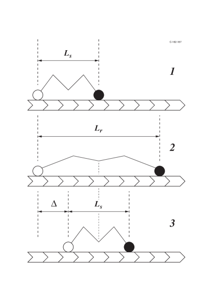
The motor model based on protein friction which was introduced in Ref. Mogilner et al. (1998), is defined as follows, compare Fig. 1. Assume that the mechanochemical cycle of the motor protein walking along the track made up of an actin filament or microtubule can be pinned down to the periodical switching between two states, and that each of these two states can be described by two motor heads connected by an effective spring representing the backbone of the motor protein between these heads. From the strained state (S), characterized by a rest length , the motor protein converges towards a relaxed state (R) with rest length , i.e., the distance between the motor heads increases. This process is slow enough to make sure that the adhesion between the motor’s ‘working head’ (white circle in Fig. 1) and track stays intact, in such a manner that asymmetric motion with respect to the track is achieved (stick). In contrast, during the fast ‘power stroke’ from the relaxed state back to the strained state after hydrolysis of ATP, the protein friction is broken and both heads move under the low Reynolds number conditions of the environment, such that both heads symmetrically approach each other and assume the rest length (slip).
This model can be cast into the two coupled Langevin equations:
| (1) | |||||
| (2) |
in which we have introduced the time-dependent friction coefficient in comparison to Ref. Mogilner et al. (1998) for convenience, to account for the cyclical attachment to the track. In Eqs. (1,2) the variable and represent the positions of the two heads of the motor molecule along the track, corresponding to the equations of motion of two coupled, overdamped oscillators. The coordinate of the idle head is associated with a viscous friction drag coefficient of order (Stokes law), where is the viscosity of water and the size of the motor protein head. The same friction acts on the working head during the fast conformational change RS, whereas during the slow process SR, it experiences the protein friction drag with coefficient Tawada and Sekimoto (1991); Leibler and Huse (1993); Jannink et al. (1996); Brokaw (1997); Jülicher et al. (1997); Imafuku et al. (1996), corresponding to a stick-slip motion of the working head. The model equations (1,2) are driven by thermal noises and , with , representing the ambient environment with correlations
| (3) |
balancing the friction terms by means of the fluctuation-dissipation theorem. We note that during the detached straining step, the role of working and idle heads may be exchanged (i.e., the motor heads may be turned around a common axis), as was recently demonstrated for kinesin motor heads Kaseda et al. (2003).
The conformational changes of the motor driven by the ATP-ADP hydrolytic cycle and the cyclical attachment to the substrate correspond to a continuous two-state Markov process for the time dependent rest length , the time dependent spring constant , and the time dependent protein friction , alternating between state R with rest length , spring constant , and protein friction and state S with rest length , spring constant , and viscous friction . The power stroke conformational transition RS driven by the ATP hydrolysis is characterized by the rate ; the relaxational conformation change SR has the rate .
The relevant biological parameters quoted in Ref. Mogilner et al. (1998), entering Eqs. (1) and (2), are: Rate of hydrolysis s-1, relaxation rate s-1, spring coefficient in relaxed state pN/nm, spring coefficient in strained state pN/nm, rest length in relaxed state nm, rest length in strained state nm, viscous drag coefficient pN s/nm, protein friction drag coefficient pN s/nm, and load force pN. For further discussion of the model and parameter choices under biological conditions we refer to ref. Mogilner et al. (1998). An important difference between the model of Mogilner at al. and the present one in Eqs. (1) and (2) is that we take during the entire duration of the strained state , while Mogilner assumes only in the first short time interval as the spring contracts (a time interval of order ; in the simulations of Ref. Mogilner et al. (1998) is taken infinitesimally small), after which the protein bonds will form and protein friction take over, . The two models will be similar if the relaxation time is of the order of .
III Analysis
In this Section, we present a solution scheme for this motor model. The results obtained are then further analyzed in the following Section.
III.1 Analytical solution
The motor equations (1) and (2) are readily analyzed by (i) solving Eq. (1) for and deriving , (ii) eliminating in Eq. (2) and setting the two expressions equal to one another. We thus obtain the following equations for and :
| (4) | |||
| (5) |
Denoting the initial velocity at time by Eq. (III.1) is readily solved by quadrature and together with Eq. (5) we obtain
| (6) | |||
| (7) |
which form the basis for our discussion.
We have introduced the renormalized load force , the renormalized noise , and the integrated spring and friction constant :
| (8) | |||
| (9) | |||
| (10) |
III.2 General properties
We note various general features of this solution. First, both the load force and the thermal noises and are renormalized by the fluctuating spring constant . Secondly, the thermal noise basically enters additively and entails thermal fluctuations of the velocities. Since the stochastic conformational changes giving rise to the fluctuations of , , and are independent of the thermal fluctuations we can in order to monitor the time dependence of the mean motor velocity with impunity average over the noise. Note that the heat bath, of course, still enters through the friction coefficients. In the long time steady state limit we can ignore the initial terms and we obtain the reduced equations for the thermally averaged velocities
| (11) | |||
| (12) |
which we proceed to discuss.
III.3 Constant spring constant and rest length
Let us first as an illustration consider the case of a constant spring length , a constant spring constant , and a constant protein friction . In this simple case and the load force is unrenormalized. We obtain
| (13) |
Here the load after a transient period drives the idle and working heads with a constant mean velocity. Defining the mobility according to
| (14) |
we infer the mobility in the absence of conformational fluctuations
| (15) |
In the absence of a load for , the mean velocity vanishes and the system does not move, i.e., we do not have motor properties. This is also a statement of the second law of thermodynamics expressing the fact that we cannot extract work from a system in thermal equilibrium. In the case of constant , constant , and constant the coupled Langevin equations describe the temporal fluctuations of a system in thermal equilibrium. The motor property is thus necessarily due to the fluctuating spring constant and fluctuating length characterizing the conformational fluctuations in combination with the cyclical attachment described by the fluctuating friction coefficient .
III.4 Fluctuating spring constant, rest length, and protein friction
The idea behind the model is that fluctuations of the spring constant () and rest length (), modelling the ATD-ADP driven conformational changes, provide an energy source. In combination with the synchronized stick-slip mechanism modelled by a fluctuating protein friction (), this process can drive the system in the absence of a force. This mechanism is modelled by the two-step Markovian process SR with relaxation rates for SR and for RS. The master equations for this process denoting the corresponding probabilities by and thus take the form:
| (16) | |||
| (17) |
with stationary solutions
| (18) | |||
| (19) |
The stationary mean value of, e.g., the spring constant, is thus given by
| (20) |
For the present purposes it turns out to be more convenient in discussing the conformational transitions to focus on the probability distributions and characterizing the residence of the system in either the strained state or the relaxed state at a time . The distribution is exponential in time and we obtain properly normalized
| (21) | |||
| (22) |
The mean values of the residence times are then given by
| (23) | |||
| (24) |
The mean value of may then be obtained as a time average:
| (25) |
in accordance with Eq. (20).
III.5 The motor property without a load
Here we establish the fundamental motor property of the model in the absence of a load. For we have from Eqs. (11) and (12),
| (26) | |||
| (27) |
At a superficial glance it looks like the motor heads move in opposite direction. However, subtracting the velocities and noting that
| (28) |
we obtain
| (29) |
Finally, assuming ergodicity (to be established later) and time averaging in combination with partial integrations we have for
| (30) | |||||
where the last step corresponds to an integration by parts (note that is monotonically increasing, and therefore ), and we conclude that the average velocities of the two heads are in fact identical: The working head and the idle head move together.
Next we derive an explicit expression for . Introducing the auxiliary fluctuating variable
| (31) |
and using the above result we obtain by adding Eqs. (26) and (27):
| (32) |
Here denotes an ensemble average with respect to the conformational fluctuations. Since , , and are governed by the same stochastic process, with the values , , , and , , in the strained and relaxed states, respectively, we obtain from the expressions for and in Eqs. (31) and (10)
| (33) | |||
| (34) | |||
| (35) | |||
| (36) |
Denoting the jump times for the transitions between the strained and relaxed state by , and assuming that the system is in a relaxed state at we have
| (37) |
and inserting in Eq. (32) we obtain
| (38) |
where . Note that the exponential term is just a more complicated way to write , which will be useful below. For even the system is in the relaxed state for with probability . Similarly for odd the motor ends in the strained state which occurs with probability . Introducing the time interval , noting that the residence distributions are statistically independent, and introducing the notation
| (39) | |||
| (40) |
the mean velocity can be expressed in terms of geometrical series,
| (41) |
or summing the series (completing ),
| (42) |
Inserting , , , and from Eqs. (19), (18), (39), and (40) we arrive at
| (43) |
First we note that the expression vanishes for thus corroborating the validity of the time average in Eq. (30) and establishing ergodicity. Finally, inserting , , , and from Eqs. (33), (34), (35), and (36) we obtain for the explicit expression for the motor velocity in the absence of a load
| (44) |
III.6 The motor property with load
We next turn to the case of a load force applied to the motor. First we establish that in the presence of the load the two heads of the motor move together with the same average velocity. From Eqs. (11) and (12) we obtain
| (45) |
Inserting from Eq. (8) and averaging over time we have, using Eq. (30):
| (46) | |||||
Performing the integrals by partial integration along the same lines as in the load-free case, the first two terms in Eq. (46) cancel and we find in the limit ,
| (47) |
i.e., the two motor heads move together with the same average velocity.
We now turn to the evaluation of the load-velocity relationship. From Eqs. (11) and (12) and inserting we have
| (48) | |||
| (49) |
From the synchronization of the stochastic processes we obtain the identity
| (50) |
and therefore
| (51) |
Inserting into Eqs. (48) and (49) and averaging
| (52) | |||||
| (53) | |||||
The first integral in Eqs. (52) and (53) has the form
| (54) |
and is performed by breaking up the integration over in the exponents and averaging over the time segments yielding again a geometrical series in terms of . We obtain as an intermediate result
| (55) |
and performing the sum and inserting and from Eqs. (39) and (40),
| (56) |
The second integral has the structure
| (57) |
and was performed in the load-free case in Eqs. (38) to (43). We found
| (58) |
It is again convenient to introduce the mobility according to the relation
| (59) |
and we obtain inserting for , or for
| (60) | |||||
IV Discussion
In this Section, we examine more closely our results derived above, and compare them to the analysis in Ref. Mogilner et al. (1998).
IV.1 Free motor
Let us first examine the simple motor properties in the absence of a cargo, i.e., for . Here the expression in Eq. (44) is at variance with the heuristic expression given by Mogilner Mogilner et al. (1998),
| (61) |
which is solely based on the reaction rates, neglecting the internal dynamics of the motor. To compare the expression for the present model, Eq. (44) we introduce the dimensionless parameters
| (62) |
and
| (63) |
which express the ratio between the spring relaxation times, and , and the residence times Eqs. (23) in states and , respectively. In terms of these parameters we obtain
| (64) |
The correction factor to the heuristic velocity given by Mogilner et al. is clearly smaller than 1, but approaches 1 in the limit of and , , which are exactly the conditions under which expression (61) was derived.
We note that the velocity vanishes for . In this case the attachment to the track has no effect on the friction and there is no motion. In the limit of large protein friction compared to the viscous drag coefficient, , but and/or each conformational cycle does not yield a full step of length due to incomplete spring relaxation, and the average velocity is reduced. In the limit of either or the motor comes to rest, as the relaxation rate or the hydrolysis rate become too large for the spring to change its average length. The motor would also function under conditions or , it would just move in the opposite direction.
Inserting the characteristic biological numbers from Ref. Mogilner et al. (1998) we have , , and , and the correction factor takes a value of about . This corresponds to a average velocity of . However, under different conditions, the discrepancy between the heuristic result (61) and the exact quantity (64) may become more significant.
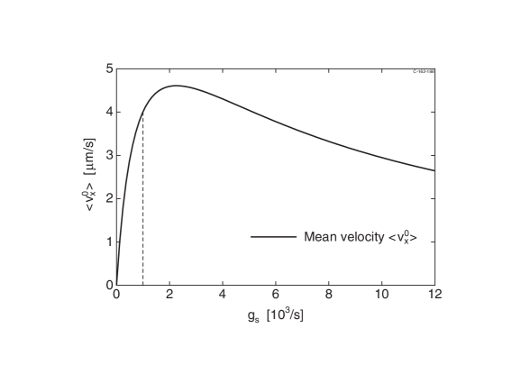
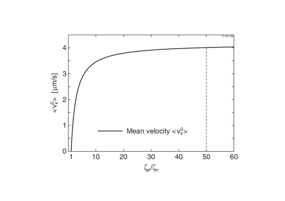
In Figs. 2 and 3, we show the dependence of the load-free velocity on the hydrolysis rate and the protein friction (all other parameters fixed at the values of Ref. Mogilner et al. (1998)). Accordingly, with respect to these values the model motor velocity is close to optimum. The maximum in the -dependence shows the interplay between on and off-rates in the protein friction model, whereas the final plateau in the -dependence indicates the above-mentioned saturation, i.e., the motor still works for extremely large values of , as long as and/or do not increase to high values, as well. We note that, as expected, the velocity goes to zero for vanishing hydrolysis rate, and when the protein friction approaches .
IV.2 Motor carrying a load
In the case of a load or cargo we proceed to discuss the expression for the motor mobility in Eq. (60), which can be rewritten in the more convenient form
| (65) |
In the further discussion of the mobility it is convenient to introduce the dimensionless parameters in Eqs. (62) and (63). The expression (65) can then be reduced to the form
| (66) |
Let us investigate this expression in some limiting cases: (i) In the absence of fluctuations, i.e., the case of a constant spring constant and rest length, in the relaxed state R, the protein friction is locked onto , and we have , and . By inspection of Eq. (66) we then obtain the mobility , as discussed in Sec. IIIb. (ii) Similarly, in the strained state S, the protein friction is locked onto , , , and , and we obtain the mobility . (iii) Finally, in the case , we immediately find , as is also evident from the model equations (1,2). Interpolating between the limiting cases (i) and (ii) above, we introduce the average mobility according to
| (67) |
and the mobility in Eq. (66) takes the form
| (68) |
Inserting the characteristic biological numbers of Mogilner et al.Mogilner et al. (1998): , , , and , we obtain the average mobility nm/(s pN), while the correction factor in Eq. (68) is , i.e., very close to 1. Hence, this gives rise to the ratio
| (69) |
in comparison with the value estimated in Ref. Mogilner et al. (1998):
| (70) |
The origin of the discrepancy between the present result and that of Ref. Mogilner et al. (1998) is the slight difference between the models. In the strained state Ref. Mogilner et al. (1998) operates with two characteristic times, that of conversion, i.e., the residence time Eq. (23) , and the time of the restoration of bonds between the motor working head and the groove, which is much smaller. In the present model the two times are assumed equal, corresponding to the assumption that the spring relaxation is initiated when the working head becomes attached to the groove again. From a physical point of view this is equally possible, but implies that the motor spends much shorter times in state S than in state R, or , i.e., and , and the motor becomes much more volatile to the local force during these periods.
From the mobility and the zero-load velocity , we obtain the stall force
| (71) |
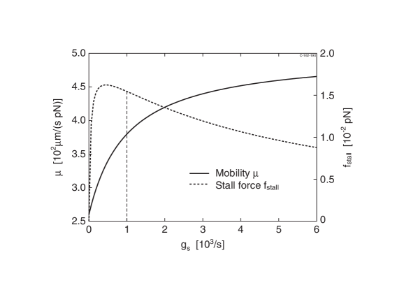
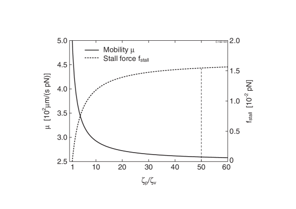
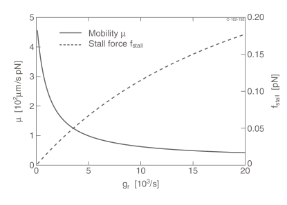
In Figs. 4 and 5 we have on the same plots depicted the values of the mobility and the stall force versus the hydrolysis rate and the protein friction . We note that the stall force exhibits a maximum as function of close to the parameter values chosen in our calculations, whereas the mobility is close to saturation. Similarly, as function of , the stall force is close to its maximum value, whereas the mobility does not change much within the chosen plot range (note that the ordinate does not reach the origin). In general, we observe that due to the particular dependence of on the model parameters, its value varies relatively weakly within large intervals for the individual parameter values. In Fig. 6 we have depicted the mobility and stall force as functions of the rate of relaxation . For large we obtain a stall force of the order pN, which is in the biological range.
V Summary and Conclusion
In this paper we have by analytical means solved a molecular motor model proposed by Mogilner et al. Mogilner et al. (1998). This model represents a robotic motor solely based on an effective static friction interaction between motor and its support (track). From the underlying Langevin equations, which represent the synchronized dichotomous processes of friction, effective spring constant and distance between the motor heads, we obtain explicit expressions for the load-free motor velocity, the mobility of the motor, and the stall force. Whereas the result for the load-free velocity produces a typical motor velocity of several m/s for physiologically reasonable parameters, the exact solution overestimates the mobility, leading to a value for the stall force, which is roughly two orders of magnitude smaller than physiological values and significantly smaller than the simulations results reported in Ref. Mogilner et al. (1998). This variance is associated with a difference in the stochastic dynamics underlying the analysis and the dynamical processes implied in the numerical simulation.
A likely explanation relies on the essential feature of the model, which is the decoupling of the dynamics of the motor protein-rail biopolymer interaction (chemical bonds forming and breaking) into a fast, detached process during energy consumption, and a slow relaxing process in one mechanochemical motor cycle. This purely stochastic picture leads to situations in which the motor detaches frequently, before its relaxing step is finished, and therefore the sub-cycles, which actually lend themselves to propulsion, are interrupted. Obviously, this leads to the underestimation of the stall force. In a real system, the fact that chemical bonds are established ensures that a full propulsion sub-cycle can be completed before dissociation takes place for the next loading of the internal motor ‘spring’ in parallel to hydrolysis. In comparison to the ratchet models in which the motor properties are represented by fluctuating between two different, periodic potentials, it appears that the latter rely on fewer parameters, and therefore their stall force can be adjusted better to actually observed values.
We finally should like to emphasize that the obtained exact results allow for an exact and detailed study of the dependence of the motor characteristics on the various parameters without invoking numerical simulations. Additional features such as the low likelihood for detaching from the rail during the forward-motion, could be incorporated into the model and still be solved explicitly, using the solution schemes developed here. We therefore believe that this study leads to a better understanding of molecular motor models.
Acknowledgements.
We should like to thank John Hertz for very constructive discussions.References
- Howard (1997) J. Howard, Nature 389, 561 (1997).
- Alberts et al. (1994) B. Alberts, K. Roberts, D. Bray, J. Lewis, M. Raff, and J. D. Watson, Molecular Biology of the Cell (Garland, New York, 1994).
- Reimann (2001) P. Reimann, Physics report 77, 993 (2001).
- Woledge et al. (1985) R. C. Woledge, N. A. Curtin, and E. Homsher, Energetic Aspects of Muscle Contraction (Academic Press, London, 1985).
- Stryer (1988) L. Stryer, Biochemistry (Freeman, San Francisco, 1988).
- Darnell et al. (1990) J. Darnell, H. Lodish, and D. Baltimore, Molecular Cell Biology (Scientific American Books, New York, 1990).
- Abeles et al. (1992) R. H. Abeles, P. A. Frey, and W. P. Jencks, Biochemistry (Jones and Bartlett, New York, 1992).
- Leibler (1994) S. Leibler, Nature 370, 412 (1994).
- Simpson et al. (2000) A. A. Simpson, Y. Z. Tao, P. G. Leiman, M. O. Badasso, Y. N. He, P. J. Jardine, N. H. Olson, M. C. Morais, S. Grimes, D. L. Anderson, et al., Nature 408, 745 (2000).
- Badoual et al. (2002) M. Badoual, F. Jülicher, and J. Prost, Proc. Natl. Acad. USA 99, 6696 (2002).
- Svoboda and Block (1994) K. Svoboda and S. M. Block, Cell 77, 773 (1994).
- Svoboda et al. (1994) K. Svoboda, P. P. Mitra, and S. M. Blockthor, Proc. Natl. Acad. USA 91, 11782 (1994).
- Kojima et al. (1997) H. Kojima, E. Muto, H. Higuchi, and T. Yanagida, Biophys. J 73, 2012 (1997).
- Higuchi et al. (1997) H. Higuchi, E. Muto, Y. Inoue, and T. Yanagida, Proc. Natl. Acad. Sci. USA 94, 4395 (1997).
- Coppin et al. (1997) C. M. Coppin, D. W. Pierce, L. Hsu, and R. D. Vale, Proc. Natl. Acad. Sci. USA 94, 8539 (1997).
- Wang et al. (1998) M. D. Wang, M. J. Schnitzer, H. Yin, R. Landick, J. Gelles, and S. M. Block, Science 282, 902 (1998).
- Mehta et al. (1999) A. D. Mehta, M. Rief, J. A. Spudich, D. A. Smith, and R. M. Simmons, Science 283, 1689 (1999).
- Strick et al. (2001) T. Strick, J.-F. Allemand, V. Croquette, and D. Bensimon, Physics Today, Oct p. 46 (2001).
- Smith et al. (2001) D. E. Smith, S. J. Tans, S. B. Smith, S. Grimes, D. L. Anderson, and C. Bustamente, Nature 413, 748 (2001).
- Fisher and Kolomeisky (1999) M. E. Fisher and A. B. Kolomeisky, Proc. Natl. Acad. Sci. 96, 6597 (1999).
- Leibler and Huse (1993) S. Leibler and D. A. Huse, J. Cell Biol. 121, 1357 (1993).
- Duke and Leibler (1996) T. Duke and S. Leibler, Biophys. J. 71, 1235 (1996).
- Magnasco (1993) M. Magnasco, Phys. Rev. Lett. 71, 1477 (1993).
- Jülicher et al. (1997) F. Jülicher, A. Ajdari, and J. Prost, Rev. Mod. Phys. 69, 1269 (1997).
- Astumian (1997) R. D. Astumian, Science 276, 917 (1997).
- Astumian and Derenyi (1999) R. D. Astumian and I. Derenyi, Biophysical Journal 77, 993 (1999).
- Astumian and Hänggi (2002) R. D. Astumian and P. Hänggi, Physics Today November, 33 (2002).
- Ambaye and Kehr (1999) H. Ambaye and K. W. Kehr, Physica 267, 111 (1999).
- Ajdari et al. (1994) A. Ajdari, D. Mukamel, L. Pelitu, and J. Prost, J. Phys. I (Paris) 4, 1551 (1994).
- Kaseda et al. (2003) K. Kaseda, H. Higuchi, and K. Hirose, Nature Cell Biol. 5, 1079 (2003).
- Vilfan et al. (1998) A. Vilfan, E. Frey, and F. Schwabl, Eur. Phys. J. B 3, 535 (1998).
- Vilfan and Duke (2003) A. Vilfan and T. Duke, Biophys. J 85, 818 (2003).
- Lee and Kardar (2001) H. Y. Lee and M. Kardar, Phys. Rev E 85, 056113 (2001).
- Mulvihill and Hyams (2001) D. P. Mulvihill and J. S. Hyams, Nature Cell Biol. 3, E1 (2001).
- Pelham and Chang (2002) R. J. Pelham and F. Chang, Nature 419, 82 (2002).
- von Smoluchowski (1912) M. von Smoluchowski, Physikal. Zeitschr. 13, 1069 (1912).
- Feynman et al. (1963) R. P. Feynman, R. B. Leighton, and M. Sands, The Feynman Lectures on Physics (Addison-Wesley, Reading, MA, 1963).
- Huxley (1957) A. F. Huxley, Prog. Biophys. 7, 255 (1957).
- Kettner et al. (2000) C. Kettner, P. Reimann, P. Hänggi, and F.Müller, Phys. Rev. E. 61, 312 (2000).
- Matthias and Müller (2003) S. Matthias and F. Müller, Nature 424, 53 (2003).
- Tawada and Sekimoto (1991) K. Tawada and K. Sekimoto, J. Theor. Biol. 150, 193 (1991).
- Jannink et al. (1996) G. Jannink, B. Duplantier, and J. L. Sikorav, Biophysical J. 71, 451 (1996).
- Brokaw (1997) C. J. Brokaw, Biophysical J. 73, 938 (1997).
- Imafuku et al. (1996) Y. Imafuku, Y. Y. Toyoshima, and K. Tawada, Biophysical J. 70, 878 (1996).
- Mogilner et al. (1998) A. Mogilner, M. Mangel, and R. J. Baskin, Phys. Lett. A 237, 297 (1998).