11institutetext: Service de Physique Théorique, Centre d’Études de Saclay, 91191 Gif-sur-Yvette Cedex, France
11email: mallick@spht.saclay.cea.fr
22institutetext: Institut de Recherche sur les Phénomènes Hors Équilibre, Université de Provence,
49 rue Joliot-Curie, BP 146, 13384 Marseille Cedex 13, France
22email: marcq@irphe.univ-mrs.fr

Stability analysis of a noise-induced Hopf bifurcation

Kirone Mallick 11    Philippe Marcq 22
(August 8, 2003)
Abstract

We study analytically and numerically the noise-induced transition between an absorbing and an oscillatory state in a Duffing oscillator subject to multiplicative, Gaussian white noise. We show in a non-perturbative manner that a stochastic bifurcation occurs when the Lyapunov exponent of the linearised system becomes positive. We deduce from a simple formula for the Lyapunov exponent the phase diagram of the stochastic Duffing oscillator. The behaviour of physical observables, such as the oscillator’s mean energy, is studied both close to and far from the bifurcation.

pacs:
05.40.-aFluctuation phenomena, random processes, noise, and Brownian motion and 05.10.GgStochastic analysis methods (Fokker-Planck, Langevin, etc.) and 05.45.-aNonlinear dynamics and nonlinear dynamical systems

1 Introduction

The stability of a dynamical system can be strongly affected by the presence of uncontrolled perturbations such as random noise lefever . Noise-induced bifurcations are of primary interest in many fields of applied mathematics and physics and occur in various experimental contexts, as for instance: electronic circuits strato , mechanical oscillators landaMc , laser physics lefever , surface waves fauve , thermal and electrohydrodynamic convection in fluids or liquid crystals kramer1 ; kramer2 ; behn and diffusion in random media frisch . In nonlinear dynamical systems, the interplay of noise and nonlinearity may produce unusual phenomena: noise can shift the bifurcation threshold from one phase to another luecke , it can induce new phase-transitions in spatially-extended systems vandenb1 , or create spatial patterns vandenb2 (for a recent review see toral ).

One of the simplest systems that may serve as a paradigm for noise-induced transitions is the nonlinear oscillator with parametric noise lindenberg ; landa ; drolet , i.e., with a frequency that fluctuates randomly with time around a given mean value bourret ; bourretFrisch . In a recent work philkir1 ; philkir2 , we studied the time asymptotic behaviour of such an oscillator in the small damping limit. We showed that physical observables grow algebraically with time until the dissipative time scale is reached; then the system settles into an oscillatory state described by a stationary probability distribution function (PDF) of the energy $E$: the zero equilibrium point ($E=0$) is unstable in the small damping limit. In the present work, we investigate the stability of the origin for arbitrary damping rate and noise strength.

For random dynamical systems, it was recognized early on that various ‘naive’ stability criteria bourret ; bourretFrisch , obtained by linearizing the dynamical equation around the origin, lead to ambiguous results. (This is in contrast with the deterministic case for which the bifurcation threshold is obtained without ambiguity by studying the eigenstates of the linearized equations manneville .) In fact, it was conjectured in bourretFrisch and proved in lindenberg3 that, in a linear oscillator with arbitrarily small parametric noise, all moments beyond a certain order diverge in the long time limit. Thus, any criterion based on finite mean displacement, momentum, or energy of the linearized dynamical equation is not adequate to insure global stability: the bifurcation threshold of a nonlinear random dynamical system cannot be determined simply from the moments of the linearized system. In practice, the transition point is usually calculated in a perturbative manner by using weak noise expansions landaMc ; luecke ; landa ; drolet .

In the present work, we shall obtain in a non-perturbative manner the bifurcation threshold of a stochastic Duffing oscillator with multiplicative, Gaussian white noise. We use a technique described in philkir1 where the stochastic dynamical equations are expressed in terms of energy-angle variables. Thanks to a detailed analysis of the associated Fokker-Planck equation, we shall show that the bifurcation occurs precisely where the Lyapunov exponent of the linear oscillator changes sign. This finding is confirmed by numerical simulations. The stability of the fixed point $E=0$ of the (nonlinear) Duffing oscillator with parametric noise is deduced, in this sense, from the linearized dynamics. We shall also derive the scaling behaviour of physical observables in the vicinity of the bifurcation with respect to the distance to threshold. Finally, we study the behaviour of observables far from the bifurcation, in the small damping or strong noise limit.

A rigorous mathematical theory of random dynamical systems has been recently developed and theorems relating the stability of the solution of a stochastic differential equation to the sign of Lyapunov exponents have been proved arnold . In the present work, we do not rely upon the sophisticated tools of the general mathematical theory but follow an intuitive approach, easily accessible to physicists, based upon a factorisation hypothesis of the stationary PDF in the limit of small and large energies.

This article is organized as follows. In Section 2, we define the system considered, present the relevant phenomenology, and introduce energy-angle variables for the stochastic Duffing oscillator. We study the stationary PDF of the energy in Section 3. In Section 4, we derive the stability criterion for the stochastic Duffing oscillator and obtain its phase diagram. In Section 5, we perform a local analysis of the physical observables in the vicinity of and far from the bifurcation threshold. Section 6 is devoted to some concluding remarks. In Appendix A, we prove some useful identities satisfied by the Lyapunov exponent. In Appendix B, an explicit formula for the Lyapunov exponent is derived.

Refer to caption
Refer to caption
Refer to caption
Figure 1: Phase plane plots of a typical trajectory of the noisy Duffing oscillator. Eq. (4) is integrated numerically with a time step $\delta t=5\ 10^{-4}$. (a) $\alpha=0.5$, $\Delta=20$, $10\leq t\leq 100$; (b) $\alpha=2.0$, $\Delta=20$, $t\leq 100$; (c) $\alpha=2.0$, $\Delta=60$, $10\leq t\leq 100$. Early-time relaxation towards noisy oscillations has been omitted for clarity in cases (a) and (c). The trajectory spirals down towards the globally stable origin in case (b).

2 The Duffing oscillator with multiplicative white noise

2.1 Notations and phenomenology

A nonlinear oscillator with a randomly varying frequency due to external noise can be described by the following equation

$$\frac{\mathrm{d}^{2}x}{\mathrm{d}t^{2}}+\gamma\frac{\mathrm{d}x}{\mathrm{d}t}+(\omega^{2}+\xi(t))x+\frac{\partial{\mathcal{U}}(x)}{\partial x}=0\,,$$ (1)

where $x(t)$ is the position of the oscillator at time $t$, ${\mathcal{U}}(x)$ an anharmonic confining potential and $\gamma$ the (positive) friction coefficient. The linear frequency of the oscillator has a mean value $\omega$ and its fluctuations are modeled by a Gaussian white noise $\xi(t)$ of zero mean-value and of amplitude ${\mathcal{D}}$

$\displaystyle\langle\xi(t)\rangle$ $\displaystyle=$ $\displaystyle 0\,,$
$\displaystyle\langle\xi(t)\xi(t^{\prime})\rangle$ $\displaystyle=$ $\displaystyle{\mathcal{D}}\,\delta(t-t^{\prime})\,.$ (2)

In this work, all stochastic differential equations are interpreted according to Stratonovich calculus. We shall study the Duffing oscillator with multiplicative noise, the confining potential ${\mathcal{U}}$ being given by

$${\mathcal{U}}(x)=\lambda\frac{x^{4}}{4}\,.$$ (3)

By rewriting time and amplitude in dimensionless units, $t:=\omega t$ and $x:=\lambda^{1/2}\omega^{-1}x,$ respectively, Eq. (1) becomes

$$\frac{\mathrm{d}^{2}x}{\mathrm{d}t^{2}}+\alpha\,\frac{\mathrm{d}x}{\mathrm{d}t}+x+x^{3}=x\,\Xi(t),$$ (4)

where $\Xi(t)$ is a delta-correlated Gaussian variable:

$\displaystyle\langle\Xi(t)\rangle$ $\displaystyle=$ $\displaystyle 0\,,$
$\displaystyle\langle\Xi(t)\Xi(t^{\prime})\rangle$ $\displaystyle=$ $\displaystyle\Delta\,\delta(t-t^{\prime})\,.$ (5)

The parameters

$$\alpha=\gamma/\omega\,\,\,\,\,\hbox{ and }\,\,\,\,\,\Delta={\mathcal{D}}/\omega^{3}$$ (6)

correspond to dimensionless dissipation rate and to noise strength, respectively. In the rest of this work, all physical quantities are expressed in dimensionless units.

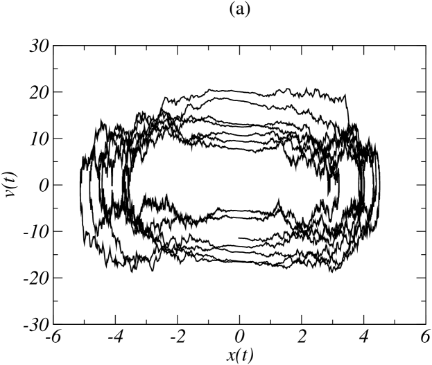
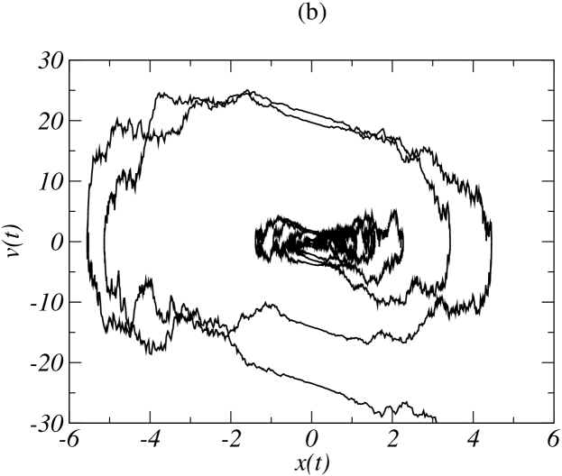
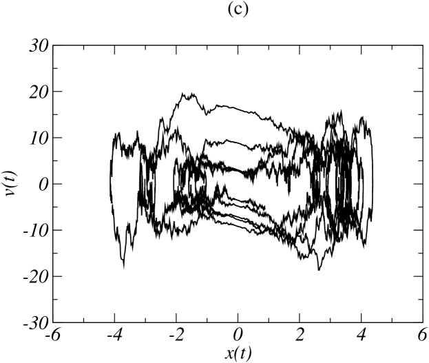
In Fig. 1, we present, for three values of the parameters, a trajectory in the phase plane $(x,v=\dot{x})$ characteristic of the oscillator’s behaviour. Here as well as for other simulations presented in this article, Eq. (4) is integrated numerically by using the one step collocation method advocated in mannella and described in detail in philkir1 . Initial conditions are chosen far from the origin, with an amplitude of order $1$. Noisy oscillations are observed for small values of the damping parameter $\alpha$ [See Fig. 1.a]. A larger value of $\alpha$ turns the origin into a global attractor for the dynamics [See Fig. 1.b]. Increasing the noise amplitude $\Delta$ at constant $\alpha$ makes the origin unstable again [See Fig. 1.c].

For all values of the parameters $(\alpha,\Delta)$, the origin $(x=\dot{x}=0)$ is a fixed point of the random dynamical system (4). Our main goal, in this work, is to investigate the stability properties of the fixed point at the origin when the control parameters vary.

2.2 Energy-angle representation of the Duffing oscillator

We now follow the method presented in philkir1 and introduce the energy-angle variables associated with the Duffing oscillator. The deterministic and undamped oscillator corresponding to Eq. (4) is an integrable dynamical system because the mechanical energy $E$, defined as

$$E=\frac{1}{2}\dot{x}^{2}+\frac{1}{2}x^{2}+\frac{1}{4}x^{4}\,,$$ (7)

is a conserved quantity. Introducing the angular variable $\phi$, the constant energy orbits of the Hamiltonian system ${\ddot{x}}+\,x+\,x^{3}=0$ are parametrized as

$\displaystyle x$ $\displaystyle=$ $\displaystyle\left(\frac{4E^{2}}{4E+1}\right)^{1/4}{\rm sd}\left(\phi\;;k\right),$ (8)
$\displaystyle\dot{x}$ $\displaystyle=$ $\displaystyle(2E)^{1/2}\frac{{\rm cn}\left(\phi\;;k\right)}{{\rm dn}^{2}\left(\phi\;;k\right)},$ (9)

where the functions sd, cn and dn are Jacobi elliptic functions abram . The elliptic modulus $k$ is a function of the energy and is given by

$$k^{2}=\frac{\sqrt{4E+1}-1}{2\sqrt{4E+1}}.$$ (10)

In the $(E,\phi)$ coordinate system, the dynamical equations for the Duffing oscillator, without noise and dissipation, become simply

$\displaystyle\dot{E}$ $\displaystyle=$ $\displaystyle 0\,,$
$\displaystyle\dot{\phi}$ $\displaystyle=$ $\displaystyle(4E+1)^{\frac{1}{4}}\,.$ (11)

We reintroduce the multiplicative noise and the dissipation terms, and obtain a system of coupled stochastic equations that describes the evolution of the energy and angle variables:

$\displaystyle\dot{E}$ $\displaystyle=$ $\displaystyle J_{E}(E,\phi)+D_{E}(E,\phi)\,\Xi(t)\,\,,$ (12)
$\displaystyle\dot{\phi}$ $\displaystyle=$ $\displaystyle J_{\phi}(E,\phi)+D_{\phi}(E,\phi)\,\Xi(t)\,\,,$ (13)

where the drift and diffusion coefficients $J_{E}$, $J_{\phi}$, $D_{E}$ and $D_{\phi}$ are defined by (see philkir1 for details of the derivation):

$\displaystyle J_{E}(E,\phi)=-2\,\alpha\,E\,\frac{{\rm cn}^{2}(\phi;k)}{{\rm dn}^{4}(\phi;k)}$ (14)
$\displaystyle D_{E}(E,\phi)=\frac{2E}{(4E+1)^{\frac{1}{4}}}\,\frac{{\rm sn}(\phi;k){\rm cn}(\phi;k)}{{\rm dn}^{3}(\phi;k)}$ (15)
$\displaystyle J_{\phi}(E,\phi)=(4E+1)^{\frac{1}{4}}+\alpha\,\frac{2E+1}{4E+1}\,\frac{{\rm sn}(\phi;k){\rm cn}(\phi;k)}{{\rm dn}^{3}(\phi;k)}$ (16)
$\displaystyle D_{\phi}(E,\phi)=-\frac{(2E+1)}{(4E+1)^{\frac{5}{4}}}\,{\rm sd}^{2}(\phi;k)$
$\displaystyle-\frac{E}{(4E+1)^{\frac{7}{4}}}{\rm sd}^{4}(\phi;k)+\frac{\alpha\,E}{(4E+1)^{\frac{3}{2}}}\,\frac{{\rm cn}(\phi;k){\rm sd}^{3}(\phi;k)}{{\rm dn}^{2}(\phi;k)}$
$\displaystyle+\frac{E}{(4E+1)^{\frac{7}{4}}}\;\frac{{\rm sn}(\phi;k){\rm cn}(\phi;k)}{{\rm dn}^{3}(\phi;k)}\,\int_{0}^{\phi}{\rm sd}^{2}(\theta;k)d\theta$
$\displaystyle-\frac{\alpha\,E}{(4E+1)^{\frac{3}{2}}}\,\frac{{\rm cn}^{2}(\phi;k)}{{\rm dn}^{4}(\phi;k)}\,\int_{0}^{\phi}{\rm sd}^{2}(\theta;k)d\theta.$ (17)

3 Analysis of the Fokker-Planck equation

Using the same notations, the Fokker-Planck equation that governs the time evolution of the probability distribution function $P_{t}(E,\phi)$ associated with the stochastic differential system (12)-(13) reads vankampen

$\displaystyle\partial_{t}P_{t}(E,\phi)$ $\displaystyle=$ $\displaystyle-\partial_{E}\left(J_{E}P\right)-\partial_{\phi}\left(J_{\phi}P\right)$ (18)
$\displaystyle+\frac{\Delta}{2}$ $\displaystyle\left[\right.\partial_{E}\left(D_{E}\partial_{E}(D_{E}P)\right)+\partial_{E}\left(D_{E}\partial_{\phi}(D_{\phi}P)\right)$
$\displaystyle+\partial_{\phi}\left(D_{\phi}\partial_{E}(D_{E}P)\right)+\partial_{\phi}\left(D_{\phi}\partial_{\phi}(D_{\phi}P)\right)\left.\right].$

The goal of this section is to determine the conditions under which there exist stationary solutions $P_{\rm{stat}}(E,\phi)$ of Eq. (18) with a non-zero mean energy. Such an extended PDF describes an oscillatory asymptotic state.

Obtaining an analytical expression of $P_{\rm{stat}}(E,\phi)$ in the general case is a daunting task. In the following, we shall perform a local analysis of Eq. (18) for small and large values of $E$. In these limiting cases, the expressions of the drift and diffusion coefficients take simpler forms. We may write, in full generality,

$$P_{\rm{stat}}(E,\phi)=P_{\rm{stat}}(\phi|E)\,{\tilde{P}}_{\rm{stat}}(E)\,,$$ (19)

where $P_{\rm{stat}}(\phi|E)$ represents, in the stationary state, the conditional probability of the angle $\phi$ at a fixed value of the energy $E$. Assuming the conditional probability $P_{\rm{stat}}(\phi|E)$ to be independent of $E$ when $E\ll 1$ and $E\gg 1$ (respectively Secs. 3.1 and 3.2), we shall derive the local behaviour of a stationary solution of the Fokker-Planck equation (18). This solution is a legitimate PDF when it is normalizable: the normalizability condition provides the location of the bifurcation graham .

3.1 Small $E$ limit: the linearized stochastic oscillator

When the oscillator’s mechanical energy $E$ is small, the position $x(t)$ and the velocity $\dot{x}(t)$ are also small: nonlinear terms may be neglected. The Duffing oscillator simplifies to a linear (harmonic) oscillator:

$$\ddot{x}+\alpha\dot{x}+x=x\;\Xi(t)$$ (20)

with $\langle\Xi(t)\Xi(t^{\prime})\rangle=\Delta\;\delta(t-t^{\prime})$. The energy now reads $E=\frac{1}{2}\,{\dot{x}}^{2}+\frac{1}{2}\,x^{2}$, and Eqs. (8) and (9) reduce to

$\displaystyle x$ $\displaystyle=$ $\displaystyle\sqrt{2E}\sin\phi\,,$ (21)
$\displaystyle\dot{x}$ $\displaystyle=$ $\displaystyle\sqrt{2E}\cos\phi\,.$ (22)

In the small $E$ limit, the elliptic modulus $k$ goes to zero, the elliptic functions reduce to circular functions abram , and the drift and diffusion coefficients simplify to

$\displaystyle J_{E}(E,\phi)$ $\displaystyle=$ $\displaystyle-2\,\alpha\,E\,\cos^{2}\phi\,$ (23)
$\displaystyle D_{E}(E,\phi)$ $\displaystyle=$ $\displaystyle 2\,E\,\sin\phi\cos\phi\,,$ (24)
$\displaystyle J_{\phi}(E,\phi)$ $\displaystyle=$ $\displaystyle 1+\alpha\sin\phi\cos\phi\,,$ (25)
$\displaystyle D_{\phi}(E,\phi)$ $\displaystyle=$ $\displaystyle-\sin^{2}\phi\,.$ (26)

Substituting the expressions (23)–(26) in Eq. (18) and integrating over $E$, we obtain an independent Fokker-Planck equation for the marginal PDF ${\tilde{P}}_{\rm{t}}(\phi)$:

$\displaystyle\partial_{t}{\tilde{P}}_{t}(\phi)$ $\displaystyle=$ $\displaystyle-\partial_{\phi}\left[(1+\alpha\sin\phi\cos\phi)\,{\tilde{P}}_{t}(\phi)\right]$ (27)
$\displaystyle+\frac{\Delta}{2}\partial_{\phi}\left[\sin^{2}\phi\,\partial_{\phi}(\sin^{2}\phi\,{\tilde{P}}_{t}(\phi))\right]\,.$

An explicit formula for the stationary angular measure ${\tilde{P}}_{\rm{stat}}(\phi)$, solution of Eq. (27), is derived in Appendix B.

We now make the hypothesis that in the small $E$ limit, the stationary conditional measure $P_{\rm{stat}}(\phi|E)$ becomes independent of $E$ and is identical to the stationary angular distribution ${\tilde{P}}_{\rm{stat}}(\phi)$ of the harmonic oscillator:

 $$\hbox{ for }\,\,\,\,\,E\ll 1\,,\,\,\,\,\,P_{\rm{stat}}(\phi|E)={\tilde{P}}_{\rm{stat}}(\phi)\,.$$ (28)

Equation (19) becomes

$$P_{\rm{stat}}(E,\phi)={\tilde{P}}_{\rm{stat}}(E){\tilde{P}}_{\rm{stat}}(\phi)\,,$$ (29)

i.e., we assume that the stationary PDF factorizes when $E\ll 1$. An exactly solvable equation for ${\tilde{P}}_{\rm{stat}}(E)$ can now be obtained by inserting expressions (23)–(26) and the identity (29) in the Fokker-Planck equation (18) and then averaging over $\phi$:

$\displaystyle\frac{\Delta}{2}\,\left\langle\sin^{2}\phi\cos^{2}\phi\right\rangle\,\partial_{E}\left(E{\tilde{P}}_{\rm{stat}}(E)\right)=$ (30)
$\displaystyle\left(\frac{\Delta}{2}\left\langle\sin^{2}\phi\,(\sin^{2}\phi-\cos^{2}\phi)\right\rangle-\alpha\left\langle\cos^{2}\phi\right\rangle\right){\tilde{P}}_{\rm{stat}}(E)\,.$

Expectation values denoted by brackets $\langle\,\rangle$ are calculated using the stationary angular measure ${\tilde{P}}_{\rm{stat}}(\phi)$. Introducing the notations:

$\displaystyle\mu(\alpha,\Delta)$ $\displaystyle=$ $\displaystyle\frac{\Delta}{2}\,\left\langle\sin^{2}\phi\cos^{2}\phi\right\rangle\,,$ (31)
$\displaystyle\Lambda(\alpha,\Delta)$ $\displaystyle=$ $\displaystyle\frac{\Delta}{2}\left\langle\sin^{2}\phi\,(\sin^{2}\phi-\cos^{2}\phi)\right\rangle-\alpha\left\langle\cos^{2}\phi\right\rangle\,,$ (32)

Eq. (30) becomes:

$$\mu\,\partial_{E}\left(E{\tilde{P}}_{\rm{stat}}(E)\right)=\Lambda\,{\tilde{P}}_{\rm{stat}}(E)\,,$$ (33)

and admits the solution:

$${\tilde{P}}_{\rm{stat}}(E)\propto E^{\frac{\Lambda}{\mu}-1}\,\,\,\,\,\hbox{ for }\,\,\,\,\,E\ll 1\,.$$ (34)

Thus, for $E\ll 1$, the PDF ${\tilde{P}}_{\rm{stat}}(E)$ behaves as a power law of the energy.

The coefficient $\mu$ is always positive, but the sign of $\Lambda$ is a function of the parameters $\alpha$ and $\Delta$. For negative values of $\Lambda$, the stationary solution (34) is not normalizable and cannot represent a PDF; the only stationary PDF solution of (18) is then a delta function centered at the origin:

$${\tilde{P}}_{\rm{stat}}(E)=\delta(E)\,\,\,\,\,\hbox{ for }\,\,\,\,\,\Lambda<0\,.$$ (35)

Thus for negative values of $\Lambda$, the origin is a global attractor for the stochastic nonlinear oscillator. Non-trivial stationary solutions exist only for $\Lambda>0$: the bifurcation threshold corresponds to values of the parameters for which $\Lambda(\alpha,\Delta)=0$.

3.2 Large $E$ limit

For very large values of $E$, the elliptic modulus $k$, defined in Eq. (10), tends to $1/\sqrt{2}$, and the drift and diffusion coefficients become

$\displaystyle J_{E}(E,\phi)$ $\displaystyle=$ $\displaystyle-2\,\alpha\,E\,\frac{\rm{cn}^{2}(\phi)}{\rm{dn}^{4}(\phi)},$ (36)
$\displaystyle D_{E}(E,\phi)$ $\displaystyle=$ $\displaystyle\sqrt{2}\,E^{3/4}\,\frac{\rm{sn}(\phi)\,\rm{cn}(\phi)}{\rm{dn}^{3}(\phi)},$ (37)
$\displaystyle J_{\phi}(E,\phi)$ $\displaystyle=$ $\displaystyle(4E)^{1/4}+\frac{\alpha}{2}\,\frac{\rm{sn}(\phi)\,\rm{cn}(\phi)}{\rm{dn}^{3}(\phi)},$ (38)
$\displaystyle D_{\phi}(E,\phi)$ $\displaystyle=$ $\displaystyle-\frac{1}{2\sqrt{2}E^{1/4}}\,\rm{sd}^{2}(\phi),$ (39)

in agreement with Eqs. (3) and (4) of philkir2 (we have omitted the elliptic modulus $1/\sqrt{2}$ for sake of simplicity). Using expressions (36) to (39) for the drift and diffusion coefficients, the stochastic equations (12) and (13) reduce, in the large $E$ limit, to

$\displaystyle\dot{E}$ $\displaystyle=$ $\displaystyle-2\,\alpha\,E\,\frac{\rm{cn}^{2}(\phi)}{\rm{dn}^{4}(\phi)}+\sqrt{2}\,E^{3/4}\,\frac{\rm{sn}(\phi)\,\rm{cn}(\phi)}{\rm{dn}^{3}(\phi)}\,\Xi(t)$ (40)
$\displaystyle\dot{\phi}$ $\displaystyle=$ $\displaystyle(4E)^{1/4}+\frac{\alpha}{2}\frac{\rm{sn}(\phi)\,\rm{cn}(\phi)}{\rm{dn}^{3}(\phi)}-\frac{\sqrt{2}}{4E^{1/4}}\rm{sd}^{2}(\phi)\,\Xi(t)$ (41)

In terms of the variable $\Omega=E^{1/4},$ Eq. (40) becomes linear and has a form similar to Ornstein-Uhlenbeck’s equation. Because the elliptic functions are bounded, $\Omega$ saturates to a value of the order of $\frac{\Delta}{\alpha}$. Thus, we deduce from Eq. (41) that the phase $\phi$ grows linearly with time. Hence, $\phi$ is a fast variable as compared to $\Omega$. Integrating out this fast variable from the Fokker-Planck equation leads to an effective stochastic dynamics for $\Omega$, as explained in detail in philkir1 . An equivalent formulation is to assume that, in the large $E$ limit, the stationary conditional probability $P_{\rm{stat}}(\phi|E)$, defined in Eq. (19), becomes uniform in $\phi$ and independent of $E$, i.e.,

 $$\hbox{ for }\,\,\,\,\,E\gg 1\,,\,\,\,\,\,P_{\rm{stat}}(\phi\,|\,E)\sim 1\,.$$ (42)

Averaging the dynamics over $\phi$ yields the following expression for the stationary PDF lindenberg ; philkir2 :

 $$\hbox{ for }\,E\gg 1,\,{\tilde{P}}_{\rm{stat}}(E)\propto E^{-1/4}\exp\left\{-\frac{8\,\alpha\,E^{1/2}}{3\,{\mathcal{M}}\,{\Delta}}\right\}\,,$$ (43)

with ${\mathcal{M}}=\frac{8}{5\pi^{2}}\Gamma\left(3/4\right)^{4}\simeq 0.3655$, $\Gamma$ being the Eulerian factorial function. A stationary solution of (18) decays as a stretched exponential and is always integrable at infinity irrespective of the values of $\alpha$ and $\Delta$.

4 Phase Diagram of the Duffing oscillator

In the long time limit, the energy of a harmonic oscillator with parametric noise (20) varies exponentially with time bourret . This behaviour is characterized by a Lyapunov exponent, defined as $\lim_{t\to\infty}\;\frac{1}{2t}\,\overline{\log E}$, where the overline means averaging over $P_{t}(E,\phi)$ hansel . [The factor $1/2$ is included for consistency with the usual definition of the Lyapunov exponent in terms of the position $x(t)$.]

In Appendix A, we prove that the coefficient $\Lambda(\alpha,\Delta)$ defined in Eq. (32) is equal to the Lyapunov exponent:

$$\Lambda(\alpha,\Delta)=\lim_{t\to\infty}\;\frac{1}{2t}\,\overline{\log E}\,.$$ (44)
Refer to caption
Figure 2: Phase diagram of the Duffing oscillator with multiplicative noise. The critical curve separates an absorbing and an oscillatory phase in the $(\alpha,\Delta)$ plane. The dashed line represents the asymptotic approximation, Eq. (47).

For the (nonlinear) Duffing oscillator, we found in Section 3 that a non-trivial stationary solution $P_{\rm{stat}}(E,\phi)$ of Eq. (18) exists only when the Lyapunov exponent $\Lambda(\alpha,\Delta)$ of the associated linear oscillator is positive. This extended PDF describes an oscillatory asymptotic state for the Duffing oscillator, as opposed to the absorbing state associated with the delta function (35). The location of the stochastic bifurcation threshold of the Duffing oscillator, which separates the two states, is given by the curve $\Lambda(\alpha,\Delta)=0$. The following explicit formula is derived in Appendix B:

$$\Lambda(\alpha,\Delta)=\frac{1}{2}\left\{\frac{\int_{0}^{+\infty}\mathrm{d}u\;{\sqrt{u}}\;e^{-\frac{2}{\Delta}\left((1-\frac{\alpha^{2}}{4})u+\frac{u^{3}}{12}\right)}}{\int_{0}^{+\infty}\frac{\mathrm{d}u}{\sqrt{u}}e^{-\frac{2}{\Delta}\left((1-\frac{\alpha^{2}}{4})u+\frac{u^{3}}{12}\right)}}-\alpha\right\}\,.$$ (45)

The transition line is determined by the relation between $\alpha$ and $\Delta$ for which the Lyapunov exponent vanishes. For a given value of $\Delta$, the critical value of the damping $\alpha=\alpha_{c}(\Delta)$ satisfies

$$\alpha_{c}={\displaystyle{\frac{\int_{0}^{+\infty}\mathrm{d}u\;{\sqrt{u}}\;\exp\left\{-\frac{2}{\Delta}\left((1-\frac{\alpha_{c}^{2}}{4})u+\frac{u^{3}}{12}\right)\right\}}{\int_{0}^{+\infty}\frac{\mathrm{d}u}{\sqrt{u}}\exp\left\{-\frac{2}{\Delta}\left((1-\frac{\alpha_{c}^{2}}{4})u+\frac{u^{3}}{12}\right)\right\}}}.}$$ (46)

The critical curve $\alpha=\alpha_{c}(\Delta)$ [Eq. (46)] is represented in Fig. 2. It separates two regions in parameter space: for $\alpha<\alpha_{c}$ (resp. $\alpha>\alpha_{c}$) the Lyapunov exponent is positive (resp. negative), the stationary PDF is an extended function (resp. a delta distribution) of the energy, the origin is unstable (resp. stable). For a detailed analytical study, we must now distinguish three cases corresponding to an underdamped ($\alpha_{c}<2$), critically damped ($\alpha_{c}=2$) and overdamped ($\alpha_{c}>2$) oscillator.

4.1 Underdamped oscillator

The case $\alpha_{c}<2$ can formally be mapped onto that of a linear oscillator with no damping. In terms of the variables $v=u\left[1-\frac{\alpha_{c}^{2}}{4}\right]^{-1/2}$ and $\Delta_{<}=\Delta\left[1-\frac{\alpha_{c}^{2}}{4}\right]^{-3/2}$, Eq. (46) reads

$\displaystyle\alpha_{c}$ $\displaystyle=$ $\displaystyle\left[1-\frac{\alpha_{c}^{2}}{4}\right]^{1/2}\;\frac{\int_{0}^{+\infty}\mathrm{d}v\,{\sqrt{v}}\,\exp\left\{-\frac{2}{\Delta_{<}}\left(v+\frac{v^{3}}{12}\right)\right\}}{\int_{0}^{+\infty}\frac{\mathrm{d}v}{\sqrt{v}}\exp\left\{-\frac{2}{\Delta_{<}}\left(v+\frac{v^{3}}{12}\right)\right\}}$
$\displaystyle=$ $\displaystyle\frac{\Delta_{<}}{2}\;\left[1-\frac{\alpha_{c}^{2}}{4}\right]^{1/2}\;\frac{\sum_{n=0}^{\infty}\frac{(-1)^{n}}{n!}\,\Gamma\left(3n+\frac{3}{2}\right)\,\left(\frac{\Delta_{<}^{2}}{48}\right)^{n}}{\sum_{n=0}^{\infty}\frac{(-1)^{n}}{n!}\,\Gamma\left(3n+\frac{1}{2}\right)\,\left(\frac{\Delta_{<}^{2}}{48}\right)^{n}}\,.$

Retaining only the lowest order term in this series, we obtain the limiting behaviour of the critical curve $\alpha_{c}(\Delta)$, for small values of $\alpha$ and $\Delta$:

$$\alpha_{c}=\frac{\Delta}{4}.$$ (47)

The change of variables used here breaks down at $\alpha_{c}=2$, we shall therefore consider this case separately.

4.2 Critically damped oscillator

For a critically damped oscillator, we substitute $\alpha_{c}=2$ in Eq. (46) and obtain

$$2=\frac{\int_{0}^{+\infty}\mathrm{d}u\,{\sqrt{u}}\,\exp\left(-\frac{u^{3}}{6\Delta_{c}}\right)}{\int_{0}^{+\infty}\frac{\mathrm{d}u}{\sqrt{u}}\,\exp\left(-\frac{u^{3}}{6\Delta_{c}}\right)}=(6\Delta_{c})^{1/3}\,\frac{\Gamma\left(\frac{1}{2}\right)}{\Gamma\left(\frac{1}{6}\right)}\,.$$ (48)

Thus, the critical noise amplitude $\Delta_{c}$ for $\alpha_{c}=2$ is

$$\Delta_{c}=\frac{4}{3}\;\frac{\Gamma\left(\frac{1}{6}\right)^{3}}{\pi^{3/2}}\simeq 41.2969...,$$ (49)

and the expression (45) for the Lyapunov exponent reduces to

$$\Lambda=\left(\frac{\Delta}{\Delta_{c}}\right)^{1/3}-1\,.$$ (50)

4.3 Overdamped oscillator

For $\alpha_{c}>2$, we define $v=u\left[\frac{\alpha_{c}^{2}}{4}-1\right]^{-1/2}$ and $\Delta_{>}=\Delta\left[\frac{\alpha_{c}^{2}}{4}-1\right]^{-3/2}$. Equation (46) then becomes

$\displaystyle\alpha_{c}\,\left[\frac{\alpha_{c}^{2}}{4}-1\right]^{-1/2}$ $\displaystyle=$ $\displaystyle\frac{\int_{0}^{+\infty}\mathrm{d}v\,{\sqrt{v}}\,e^{-\frac{2}{\Delta_{>}}\left(-v+\frac{v^{3}}{12}\right)}}{\int_{0}^{+\infty}\frac{\mathrm{d}v}{\sqrt{v}}e^{-\frac{2}{\Delta_{>}}\left(-v+\frac{v^{3}}{12}\right)}}$
$\displaystyle=$ $\displaystyle(6{\Delta_{>}})^{1/3}\;\frac{\sum_{n=0}^{\infty}\frac{1}{n!}\Gamma\left(\frac{2n+3}{6}\right)\left(\frac{48}{\Delta_{>}^{2}}\right)^{n/3}}{\sum_{n=0}^{\infty}\frac{1}{n!}\,\Gamma\left(\frac{2n+1}{6}\right)\left(\frac{48}{\Delta_{>}^{2}}\right)^{n/3}}$

When $\alpha_{c}\to\infty$, the left hand side of Eq. (4.3) the previous equation converges to 2 and ${\Delta_{>}}$ tends to a limiting value ${\cal K}$ that we computed numerically: ${\cal K}\simeq 28.337$. Thus, in the large $\alpha_{c}$ limit, we find the following relation between $\alpha_{c}$ and $\Delta$

$$\Delta\simeq{\cal K}\,\left[\frac{\alpha_{c}^{2}}{4}-1\right]^{3/2}\simeq\frac{{\cal K}}{8}\,\alpha_{c}^{3}\simeq 3.54\,\alpha_{c}^{3}.$$ (52)

When $\alpha_{c}\to 2^{+}$, the left hand side of Eq. (4.3) increases to infinity. Retaining only the leading order term of the series, we obtain

$$2\,\left[\frac{\alpha_{c}^{2}}{4}-1\right]^{-1/2}=(6{\Delta_{>}})^{1/3}\frac{\Gamma(1/2)}{\Gamma(1/6)}\,.$$ (53)

This equation is consistent with Eq. (49).

5 Physical observables

The goal of this section is to determine how physical observables, such as the energy and the position of the oscillator, scale near the bifurcation threshold as well as far from it. The agreement between analytical calculations and numerical simulations will validate the assumptions made in Section 3 concerning the behaviour of the conditional PDF $P_{\rm{stat}}(\phi|E)$ for small and large values of $E$.

Let us first of all review the results obtained in Section 3. For parameter values such that $\Lambda<0$, we demonstrated that ${\tilde{P}}_{\rm{stat}}(E)=\delta(E)$: the origin is a global attractor of the dynamics. Conversely, when $\Lambda>0$, the origin becomes unstable. The stationary measure of the energy is then an extended function: it behaves as a power law for small values of $E$ [see Eq. (34)], and decreases as a stretched exponential for large values of $E$ [see Eq. (43)]:

$\displaystyle\hbox{ for }\,\,E\ll 1\,,\,\,\,{\tilde{P}}^{<}_{\rm{stat}}(E)$ $\displaystyle=$ $\displaystyle AE^{\frac{\Lambda}{\mu}-1}\,,$
$\displaystyle\hbox{ for }\,\,E\gg 1\,,\,\,\,{\tilde{P}}^{>}_{\rm{stat}}(E)$ $\displaystyle=$ $\displaystyle BE^{-\frac{1}{4}}\exp\left\{-\frac{8\,\alpha\,E^{1/2}}{3\,{\mathcal{M}}\,{\Delta}}\right\}\,.$ (54)

The precise values of $A$ and $B$ can only be obtained by solving the full Fokker-Planck equation (18), and matching the two asymptotic expressions in the intermediate regime $E\simeq 1$.

5.1 Behaviour in the vicinity of the bifurcation
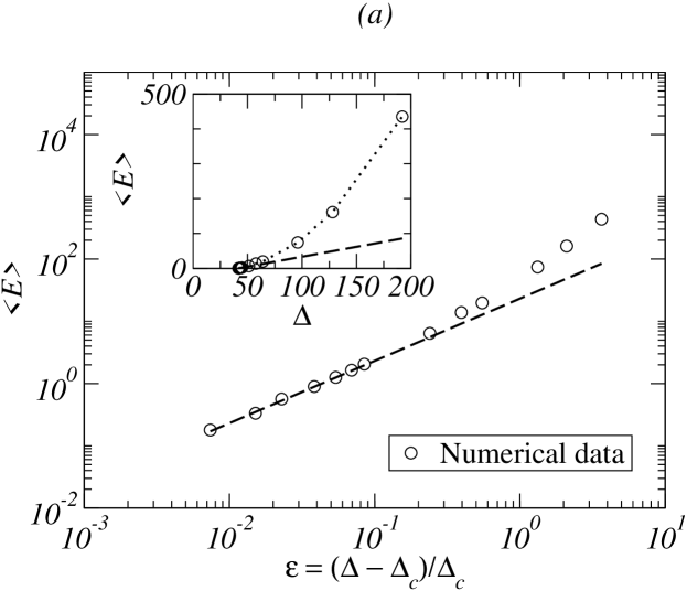
Refer to caption
Refer to caption
Figure 3: Scaling behaviour of physical observables of the stochastic Duffing oscillator in the vicinity of the bifurcation threshold as a function of the reduced control parameter $\varepsilon=(\Delta-\Delta_{c})/\Delta_{c}$. (a) Average energy; (b) Variance of the position. Dashed lines corresponding to a linear function of $\varepsilon$ are drawn to guide the eye. The corresponding linear-linear graphs are shown as insets. Eq. (4) is integrated numerically for $\alpha=2$, with a time step $\delta t=5\ 10^{-4}$. The threshold value is given by Eq. (49): $\Delta_{c}(2)\simeq 41.3$. Ensemble averages are computed over $10^{3}$ realisations.
Refer to caption
Figure 4: Scaling behaviour of the mean energy of the general nonlinear oscillator in the vicinity of the bifurcation threshold as a function of the reduced control parameter $\varepsilon=(\Delta-\Delta_{c})/\Delta_{c}$. Dashed lines indicating a linear dependence in $\varepsilon$ are drawn to guide the eye. Eq. (1) is integrated numerically for $\alpha=2$, and with ${\mathcal{U}}(x)=x^{2n}/(2n)$, $n=2$, $3$ and $4$. Data obtained for $n=2$ are the same as in Fig. 3. The time step is $\delta t=5\ 10^{-4}$; ensemble averages are computed over $10^{3}$ realisations.

For a given value of the damping rate $\alpha$, let us choose the noise strength $\Delta$ such that $0<\Delta-\Delta_{c}(\alpha)\ll 1$. In this case, the parameters of the system are tuned just above the bifurcation threshold and the Lyapunov exponent is slightly positive: $0<\Lambda\ll 1$. The stationary PDF is an extended function but, as can be inferred from Eq. (54), most of its mass is concentrated in the vicinity of $E=0$. Therefore, a good approximation of the stationary PDF is obtained by taking it equal to ${\tilde{P}}^{<}_{\rm{stat}}(E)$ over a finite interval in the vicinity of 0 (e.g., $0\leq E\leq E_{0}$), and equal to zero outside this interval. The mean value of the energy is given by:

$$\langle E\rangle_{\mathrm{stat}}\simeq\frac{\int_{0}^{E_{0}}E^{\frac{\Lambda}{\mu}}\mathrm{d}E}{\int_{0}^{E_{0}}E^{\frac{\Lambda}{\mu}-1}\mathrm{d}E}\propto E_{0}\,\frac{\Lambda}{\mu}\,.$$ (55)

If we now take into account that: $(i)$ $\Lambda(\alpha,\Delta_{c}(\alpha))=0$; and $(ii)$ the Lyapunov exponent and the coefficient $\mu$ are regular functions of the noise strength $\Delta$ when $\Delta\neq 0$, we obtain from Eq. (55)

$$\langle E\rangle_{\mathrm{stat}}\propto\Lambda(\alpha,\Delta)-\Lambda(\alpha,\Delta_{c})\propto(\Delta-\Delta_{c})\,,$$ (56)

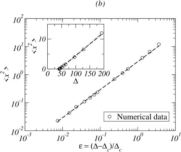
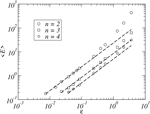
where the last identity is obtained by a Taylor expansion of $\Lambda$ for $\Delta$ close to $\Delta_{c}$. This result is confirmed by numerical simulations [See Fig. 3.a]. A similar reasoning shows that $\langle E\rangle_{\mathrm{stat}}$ scales linearly with $\alpha-\alpha_{c}(\Delta)$ at fixed noise strength $\Delta$.

Let us now consider the variance of the oscillator’s position close to the bifurcation. Using Eqs. (21) and (29), we find

$\displaystyle\langle x^{2}\rangle_{\mathrm{stat}}$ $\displaystyle=$ $\displaystyle\iint P_{\mathrm{stat}}(E,\phi)\,2E\sin^{2}\phi\;\mathrm{d}E\,\mathrm{d}\phi$ (57)
$\displaystyle=$ $\displaystyle 2\,\langle\sin^{2}\phi\rangle\,\langle E\rangle_{\mathrm{stat}}$
$\displaystyle\propto$ $\displaystyle(\Delta-\Delta_{c})\,.$

The variance of the position scales linearly with the distance to threshold [See Fig. 3.b]. Using a similar argument, one also finds that $\langle v^{2}\rangle_{\mathrm{stat}}\propto(\Delta-\Delta_{c})$.

As seen in Fig. 4 the linear scaling (56) of the energy with respect to the distance to threshold is observed for ${\mathcal{U}}(x)\propto x^{2n}$, $n=2$, $3$ and $4$, where $\Delta_{c}(\alpha)$ is always given by $\Lambda(\alpha,\Delta_{c}(\alpha))=0$. The threshold is independent of the nonlinearity involved in the confining potential ${\mathcal{U}}$ appearing in Eq. (1), because the local expression ${\tilde{P}}^{<}_{\rm{stat}}(E)$ of the stationary PDF in the vicinity of $E=0$ is obtained from the linearized stochastic differential equation. The observed dependence of the constant of proportionality in Eq. (56) upon the stiffness of the anharmonic potential remains to be understood.

Refer to caption
Figure 5: Scaling behaviour of the mean energy of the general nonlinear oscillator far from the bifurcation as a function of the parameter $\Delta/\alpha$. Eq. (1) is integrated numerically with ${\mathcal{U}}(x)=x^{2n}/(2n)$, $n=2$, $3$ and $4$. Dashed lines correspond to the predicted scaling (5.2), with a scaling exponent $n/(n-1)=2$, $3/2$ and $4/3$. The time step is $\delta t=5\ 10^{-4}$; ensemble averages are computed over $10^{3}$ realisations.

5.2 Scaling far from the bifurcation

We shall now study the scaling of the physical observables far from the bifurcation point. This situation is encountered, for instance, when the damping rate is vanishingly small for a given noise strength. The Lyapunov exponent is then a finite, strictly positive, number. When $\alpha\to 0$, most of the mass of the stationary PDF is concentrated at large values of $E$ as can be seen from Eq. (54). Thus, a satisfactory approximation of the stationary PDF is to assume it to be identical to the expression ${\tilde{P}}^{>}_{\rm{stat}}(E)$ for all $E$. After a suitable normalisation, we find

$${\tilde{P}}_{\rm{stat}}(E)=\frac{1}{2E\Gamma\left(3/2\right)}\left(\frac{8\,\alpha\,E^{1/2}}{3\,{\mathcal{M}}\,{\Delta}}\right)^{3/2}\exp\left\{-\frac{8\,\alpha\,E^{1/2}}{3\,{\mathcal{M}}\,{\Delta}}\right\},$$ (58)

with the numerical factor ${\mathcal{M}}$ defined in Eq. (43). In this low damping regime, we recover, as expected, the results derived in Refs. philkir1 ; philkir2 . The average energy is readily obtained from Eq. (58)

$$\langle E\rangle_{\rm{stat}}=\frac{135}{256}\,{\mathcal{M}}^{2}\,\left(\frac{{\Delta}}{\alpha}\right)^{2}\simeq 0.070\left(\frac{{\Delta}}{\alpha}\right)^{2}\,.$$ (59)

This result is at variance with the usual equilibrium fluctuation-dissipation theorem ($\langle E\rangle_{\mathrm{eq}}\propto{\Delta}/\alpha$); yet this is not a contradiction since Eq. (4) models a system out of equilibrium.

Far from the bifurcation threshold, the scaling behaviour depends strongly on the stiffness of the potential ${\mathcal{U}}$. If we take ${\mathcal{U}}(x)\propto x^{2n}$, Eq. (59) can be generalized to philkir2

$\displaystyle\langle E\rangle_{\rm{stat}}=$ $\displaystyle\frac{1}{2n}\;\frac{\Gamma\left(\frac{3n+1}{2(n-1)}\right)}{\Gamma\left(\frac{n+1}{2(n-1)}\right)}$
$\displaystyle\left((n-1)\;\frac{\Gamma\left(\frac{3}{2n}\right)\;\Gamma\left(\frac{3n+1}{2n}\right)}{\Gamma\left(\frac{1}{2n}\right)\;\Gamma\left(\frac{3n+3}{2n}\right)}\right)^{\frac{n}{n-1}}\;\left(\frac{{\Delta}}{\alpha}\right)^{\frac{n}{n-1}}\,.$

This prediction is again confirmed by numerical simulations [See Fig. 5].

6 Conclusion

For a deterministic Duffing oscillator with linear damping, the fixed point at the origin $(x=\dot{x}=0)$ is a global attractor: irrespective of the choice of initial conditions, the mechanical energy is totally dissipated in the long time limit and the system converges to the origin. This picture is no longer valid once the oscillator is subject to parametric noise. Indeed, the dissipative Duffing oscillator with parametric white noise undergoes a noise-induced bifurcation between: $(i)$ an absorbing state reminiscent of the deterministic system; and $(ii)$ an oscillatory state, resulting from a dynamical balance between energy dissipation and (noise-induced) energy injection. Noisy oscillations appear when the fixed point at the origin becomes unstable: this transition is thus referred to as a (forward) stochastic Hopf bifurcation. Both states may be characterized by the stationary probability distribution function of the oscillator’s mechanical energy $E$. The PDF of the absorbing state is a delta-function, whereas the oscillatory state corresponds to an extended PDF.

Our main result concerns the location of the transition point: a noise-induced bifurcation for the Duffing oscillator occurs precisely where the Lyapunov exponent of the linear oscillator with parametric noise changes sign. We emphasize that this result is genuinely non-perturbative. It results from a simple hypothesis on the behaviour of the conditional probability of the angular variable at fixed energy, valid for very small values of the energy and for arbitrary noise amplitude. This assumption is physically plausible (i.e. mean-field-like) and justified by the consequences deduced from it. Having identified the Lyapunov exponent of the stochastic linear oscillator as the important physical quantity, we give a simple analytical expression of this exponent as a function of the system’s parameters, the damping rate and the noise strength. The location of the transition line that separates the absorbing and oscillatory states of the (nonlinear) Duffing oscillator follows immediately.

Although we have considered here only a cubic oscillator with parametric Gaussian white noise, we believe that the relation between the sign of the Lyapunov exponent and the location of the noise-induced transition holds irrespective of the nonlinearity and of the nature of the noise. Finally, we demonstrate that all physical observables scale linearly with respect to the distance to threshold. Indeed, the argument we use to evaluate the mean energy $\langle E\rangle$ may be easily generalized to show that all moments $\langle E^{k}\rangle$ also scale linearly, suggesting that the concept of critical exponents is not relevant here. One would certainly like to test experimentally whether noise-induced transitions may indeed be characterized by a multifractal order parameter, at variance with the theory of equilibrium continuous transitions.

Appendix A Some useful identities for the Lyapunov exponent

In this appendix, we prove that the Lyapunov exponent, defined as $\lim_{t\to\infty}\;\frac{1}{2t}\,\overline{\log E}$, satisfies the relation (44). Using the ‘radial’ variable $\rho$ defined by

$$\rho=\frac{1}{2}\log\left(2E\right)\,,$$ (61)

we rewrite Eq. (20) as a system of nonlinear coupled stochastic equations

$\displaystyle\dot{\rho}$ $\displaystyle=$ $\displaystyle-\alpha\cos^{2}\phi+\sin\phi\cos\phi\,\Xi(t)\,,$ (62)
$\displaystyle\dot{\phi}$ $\displaystyle=$ $\displaystyle 1+\alpha\sin\phi\cos\phi-\sin^{2}\phi\,\Xi(t)\,.$ (63)

The Fokker-Planck evolution equation for the joint probability distribution $P_{t}(\rho,\phi)$ is then given by vankampen

$\displaystyle\partial_{t}P_{t}$ $\displaystyle=$ $\displaystyle\alpha\cos^{2}\phi\,\partial_{\rho}P_{t}-\partial_{\phi}\left[(1+\alpha\sin\phi\cos\phi)\,P_{t}\right]$
$\displaystyle+\frac{\Delta}{2}\left\{\right.\sin^{2}\phi\cos^{2}\phi\,\partial^{2}_{\rho\rho}P_{t}-\sin\phi\cos\phi\,\partial^{2}_{\rho\phi}\left[\sin^{2}\phi\,P_{t}\right]$
$\displaystyle-\partial_{\phi}\left[\sin^{3}\phi\cos\phi\,\partial_{\rho}P_{t}\right]+\partial_{\phi}\left[\sin^{2}\phi\,\partial_{\phi}(\sin^{2}\phi\,P_{t}\,)\right]\left.\right\}$

From Eq. (A) we derive the time evolution of the mean value $\overline{\rho}$, where the overline indicates averaging with respect to $P_{t}(\rho,\phi)$. After suitable integration by parts, we obtain

$$\frac{\rm{d}}{\rm{d}t}\overline{\rho}=-\alpha\;\overline{\cos^{2}\phi}\,+\frac{\Delta}{2}\overline{\sin^{2}\phi\,(\sin^{2}\phi-\cos^{2}\phi)}\,.$$ (65)

Similarly, we deduce the time evolution of $\overline{\log|\sin\phi|}$

$\displaystyle\frac{\rm{d}}{\rm{d}t}\overline{\log|\sin\phi|}$ $\displaystyle=$ $\displaystyle\overline{\mathrm{cotan}\,\phi}+\alpha\;\overline{\cos^{2}\phi}$ (66)
$\displaystyle-\frac{\Delta}{2}\;\overline{\sin^{2}\phi\,(\sin^{2}\phi-\cos^{2}\phi)}\,.$

From Eqs. (65) and (66), we obtain

$$\frac{\rm{d}}{\rm{d}t}\overline{\rho}=\overline{\mathrm{cotan}\,\phi}-\frac{\rm{d}}{\rm{d}t}\overline{\log|\sin\phi|}\,.$$ (67)

At large times, the PDF ${P}_{t}(E,\phi)$ reaches a stationary limit ${P}_{\rm{stat}}(E,\phi)$. Thus, when $t\to\infty$, the averages $\overline{\log|\sin\phi|}$ and $\overline{\mathrm{cotan}\,\phi}$ have finite limits, given by $\langle\log|\sin\phi|\rangle$ and $\left\langle\mathrm{cotan}\,\phi\right\rangle$, respectively, where the expectation values denoted by brackets $\langle\rangle$ are calculated by using the marginal PDF, ${\tilde{P}}_{\rm{stat}}(\phi)$. Therefore

$$\lim_{t\to\infty}\frac{\rm{d}}{\rm{d}t}\overline{\rho}=\left\langle\mathrm{cotan}\,\phi\right\rangle\,.$$ (68)

From Eqs. (61) and (68), we derive

$$\lim_{t\to\infty}\frac{1}{2t}\overline{\log E}=\lim_{t\to\infty}\frac{1}{2}\frac{\mathrm{d}}{\mathrm{d}t}\overline{\log E}=\lim_{t\to\infty}\frac{\mathrm{d}}{\mathrm{d}t}\overline{\rho}=\left\langle\mathrm{cotan}\,\phi\right\rangle\,.$$ (69)

Similarly, we take the stationary limit of Eq. (66) and obtain

$$\left\langle\mathrm{cotan}\,\phi\right\rangle=-\alpha\;\left\langle\cos^{2}\phi\right\rangle+\frac{\Delta}{2}\;\left\langle\sin^{2}\phi\,(\sin^{2}\phi-\cos^{2}\phi)\right\rangle.$$ (70)

The right hand side of this equation is nothing but $\Lambda$ [See Eq. (32)]. This concludes the derivation of Eq. (44) :

$$\lim_{t\to\infty}\frac{1}{2t}\overline{\log E}=\left\langle\mathrm{cotan}\,\phi\right\rangle=\Lambda(\alpha,\Delta)\,.$$ (71)

Appendix B Calculation of the Lyapunov exponent

Expressions for the Lyapunov exponent have been available for a long time in the literature hansel , but they are rather unwieldy. In a recent article about the quantum localisation problem tessieri , an expression for the localisation length is derived: it is shown to be identical to the inverse Lyapunov exponent of the linear oscillator with parametric noise and zero damping. In this appendix, we generalize the calculation of tessieri to the dissipative case and derive a particularly simple formula for the Lyapunov exponent.

Since $\Lambda=\langle\mathrm{cotan}\phi\rangle$ [See Eq. (71)], we introduce the auxiliary variable $z$ defined as

$$z=\dot{x}/x=\mathrm{cotan}\,\phi\,.$$ (72)

Then, equation (20) becomes

$$\dot{z}+1+\alpha\;z+z^{2}=\Xi(t)\,.$$ (73)

The stationary Fokker-Planck equation associated with Eq. (73) is given by

$$\frac{\Delta}{2}\;\frac{\rm{d}}{\rm{d}z}P_{\rm{stat}}=-(1+\alpha z+z^{2})P_{\rm{stat}}+J\,,$$ (74)

where we have introduced the stationary current $J$. The solution of this equation is found by the method of the variation of constants:

$$P_{\rm{stat}}(z)=\frac{1}{N}\int_{-\infty}^{z}\exp\left\{\frac{2}{\Delta}(\Phi(y)-\Phi(z))\right\}\mathrm{d}y,$$ (75)

where $\Phi(y)=y+\frac{\alpha}{2}y^{2}+\frac{1}{3}y^{3}$. Writing $\int_{-\infty}^{\infty}P_{\rm{stat}}(z)\;\mathrm{d}z=1$, we obtain the normalisation constant $N$:

$$N=\int_{-\infty}^{+\infty}\mathrm{d}z\int_{-\infty}^{z}\mathrm{d}y\exp\left\{\frac{2}{\Delta}(\Phi(y)-\Phi(z))\right\}.$$ (76)

Following tessieri , we change the $y$ variable to $u=z-y$ in Eq. (76):

$$N=\int_{-\infty}^{+\infty}\mathrm{d}z\int_{0}^{+\infty}\mathrm{d}u\,e^{-\frac{2}{\Delta}\big{(}u-\frac{\alpha}{2}u^{2}+\frac{u^{3}}{3}+z^{2}u+z(\alpha u-u^{2})\big{)}}\,.$$ (77)

The integral over $z$ is now Gaussian, and can be evaluated before the integral over $u$. Hence, we obtain

$$N=\sqrt{\frac{\pi\Delta}{2}}\;\int_{0}^{+\infty}\frac{\mathrm{d}u}{\sqrt{u}}\,\exp\left\{-\frac{2}{\Delta}\,\left((1-\frac{\alpha^{2}}{4})u+\frac{u^{3}}{12}\right)\right\}\,.$$ (78)

The use of the identity

$${\tilde{P}}_{\rm{stat}}(\phi)\rm{d}\phi=P_{\rm{stat}}(z)\rm{d}z\,,$$ (79)

yields the stationary angular measure

$${\tilde{P}}_{\rm{stat}}(\phi)=\frac{1}{N\sin^{2}\phi}\int_{-\infty}^{\rm{cotan}\;\phi}\mathrm{d}y\;e^{\frac{2}{\Delta}\left(\Phi(y)-\Phi(\mathrm{cotan}\;\phi)\right)}\,.$$ (80)

We deduce that the Lyapunov exponent satifies

$\displaystyle\Lambda$ $\displaystyle=$ $\displaystyle\int_{0}^{\pi}{\tilde{P}}_{\rm{stat}}(\phi)\,\mathrm{cotan}\phi\,\mathrm{d}\phi$
$\displaystyle=$ $\displaystyle\frac{1}{N}\int_{-\infty}^{+\infty}\mathrm{d}z\;z\int_{-\infty}^{z}\exp\left\{\frac{2}{\Delta}(\Phi(y)-\Phi(z))\right\}\mathrm{d}y\,.$

We again change the variables from $(y,z)$ to $(u,z)$ with $u=z-y$, and obtain

$$\Lambda=\frac{1}{N}\int_{-\infty}^{+\infty}\mathrm{d}z\,z\int_{0}^{+\infty}\mathrm{d}u\,e^{-\frac{2}{\Delta}\left(u-\frac{\alpha}{2}u^{2}+\frac{u^{3}}{3}+z(\alpha u-u^{2})+z^{2}u\right)}$$ (82)

Evaluating the Gaussian integral in $z$ leads to the expression of the Lyapunov exponent given in the text

$$\Lambda(\alpha,\Delta)=\frac{1}{2}\left\{\frac{\int_{0}^{+\infty}\mathrm{d}u\;{\sqrt{u}}\;e^{-\frac{2}{\Delta}\left((1-\frac{\alpha^{2}}{4})u+\frac{u^{3}}{12}\right)}}{\int_{0}^{+\infty}\frac{\mathrm{d}u}{\sqrt{u}}e^{-\frac{2}{\Delta}\left((1-\frac{\alpha^{2}}{4})u+\frac{u^{3}}{12}\right)}}-\alpha\right\}.$$ (83)

This formula also appears in recent mathematical literature imkeller . It constitutes an exact result, obtained without approximations. We have computed numerically the Lyapunov exponent by measuring $\overline{\log E}$ in the time-asymptotic regime and thus confirmed the validity of (83).

References

  • (1) H. Horsthemke and R. Lefever, Noise Induced Transitions (Springer-Verlag, Berlin, 1984).
  • (2) R.L. Stratonovich, Topics on the Theory of Random Noise (Gordon and Breach, New York, 1963 (Vol. 1), 1967 (Vol. 2)).
  • (3) P.S. Landa and P.V.E. McClintock, Phys. Rep. 323, 1 (2000).
  • (4) R. Berthet, S. Residori, B. Roman and S. Fauve, Phys. Rev. Lett. 33, 557 (2002).
  • (5) A. Becker and L. Kramer, Phys. Rev. Lett. 73, 955 (1994); Physica D 90, 408 (1996).
  • (6) J. Röder, H. Röder and L. Kramer, Phys. Rev. E 55, 7068 (1997).
  • (7) U. Behn, A. Lange and T. John, Phys. Rev. E 58, 2047 (1998).
  • (8) U. Frisch, in Probabilistic Methods in Applied Mathematics, edited by A.T. Bharucha-Reid (Academic Press, New York, 1968).
  • (9) M. Lücke and F. Schank, Phys. Rev. Lett. 54, 1465 (1985); M. Lücke, in Noise in Dynamical Systems, Vol. 2: Theory of Noise-induced Processes in Special Applications, edited by F. Moss and P.V.E. Mc Clintock (Cambridge University Press, Cambridge, 1989).
  • (10) C. van den Broeck, J.M.R. Parrondo and R. Toral, Phys. Rev. Lett 73, 3395 (1994).
  • (11) J.M.R. Parrondo, C. van den Broeck, J. Buceta and F. Javier de la Rubia, Physica 224 A, 153 (1996).
  • (12) M. San Miguel and R. Toral, Stochastic Effects in Physical Systems, in Instabilities and Nonequilibrium Structures VI, edited by E. Tirapegui and W. Zeller (Kluwer, Dordrecht, 1997).
  • (13) V. Seshadri, B. J. West and K. Lindenberg, Physica 107 A, 219 (1981).
  • (14) P.S. Landa and A.A. Zaikin, Phys. Rev. E 54, 3535 (1996).
  • (15) F. Drolet and J. Viñals, Phys. Rev. E 57, 5036 (1998).
  • (16) R.C. Bourret, Physica 54, 623 (1971).
  • (17) R.C. Bourret, U. Frisch and A. Pouquet, Physica 65, 303 (1973).
  • (18) K. Mallick and P. Marcq, Phys. Rev. E 66, 041113 (2002).
  • (19) K. Mallick and P. Marcq, Physica 325 A, 213 (2003).
  • (20) P. Manneville, Dissipative structures and weak turbulence (Academic Press, New York, 1990).
  • (21) K. Lindenberg, V. Seshadri and B.J. West, Physica 105 A, 445 (1981).
  • (22) L. Arnold, Random Dynamical Systems (Springer-Verlag, Berlin, 1998).
  • (23) R. Mannella, in Noise in Dynamical Systems, Vol. 3: Experiments and Simulations, edited by F. Moss and P.V.E. Mc Clintock (Cambridge University Press, Cambridge, 1989).
  • (24) M. Abramowitz and I. A. Stegun, Handbook of Mathematical Functions (National Bureau of Standards, Washington, D.C., 1966).
  • (25) N.G. van Kampen, Stochastic Processes in Physics and Chemistry (North-Holland, Amsterdam, 1992).
  • (26) A. Schenzle and H. Brand, Phys. Rev. A 20, 1628 (1979).
  • (27) D. Hansel and J.F. Luciani, J. Stat. Phys. 54, 971 (1989).
  • (28) L. Tessieri and F.M. Izrailev, Phys. Rev. E 62, 3090 (2000).
  • (29) P. Imkeller and C. Lederer, Dyn. and Stab. Syst. 14, 385 (1999).