Theory of spin waves in diluted-magnetic-semiconductor quantum wells

Abstract

We present a theory of collective spin excitations in diluted-magnetic-semiconductor quantum wells in which local magnetic moments are coupled via a quasi-two-dimensional gas of electrons or holes. In the case of a ferromagnetic state with partly spin-polarized electrons, we find that the Goldstone collective mode has anomalous $k^{4}$ dispersion and that for symmetric quantum wells odd parity modes do not disperse at all. We discuss the gap in the collective excitation spectrum which appears when spin-orbit interactions are included.

I Introduction

In the emerging field of spin- or magneto-electronics,P98 ; WABDvMRCT01 the role of the spin degree-of-freedom in the properties of electronic systems is exploited in the design of new functional devices. The recognition of this additional degree of freedom suggests possibilities for electrical manipulation beyond the tool-set of conventional electronics which is based entirely on coupling to the electronic charge. The effort to generate and manipulate spin-polarized carriers in a controllable environment, preferably in semiconductors, has triggered the discovery of carrier-induced ferromagnetism SGFW86 ; O92 in diluted magnetic semiconductors (DMSs).O98 In these systems a few percent of the cations in III-V or II-VI semiconductor compounds are randomly substituted by magnetic ions, usually Mn, which have local magnetic moments. The effective coupling between these local moments is mediated by free carriers in the host semiconductor compound (holes for p-doped materials and electrons for n-doped ones) and can lead to ferromagnetic long-range order. Curie temperatures $T_{\rm c}$ in excess of 100 K have been found in bulk (Ga,Mn)As systems.O98 ; Gallagher ; Samarth

One approach to understand the magnetic and optical properties of DMSs is based on a phenomenological model of the relevant low-energy degrees of freedom.Furdyna ; Dietl94 In this picture, local $S=5/2$ spinsnote6 from Mn²⁺ ions are exchange coupled to itinerant carriers of a metallic nature. In typical samples, the density of free carriers is much smaller than the Mn ion concentration. For n-doped materials, the exchange is due to ferromagnetic s-d coupling, while for p-doped ones it is due to antiferromagnetic p-d coupling, as illustrated schematically in Fig. 1. In both cases, the free carriers are believed to mediate an effective ferromagnetic coupling between the Mn spins, which is typically stronger than the shorter-range antiferromagnetic direct exchange coupling present in undoped systems.

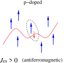
Figure 1: Schematic representation of the exchange coupling between itinerant-carrier and localized magnetic-impurity spins in n-doped and p-doped DMSs. When the local moments are parallel to each other and the band system is spin-polarized, the exchange energy can be minimized for either ferromagnetic or antiferromagnetic interactions.

The reliability of this phenomenological approach has been tested by comparing theoretical predictions with experimental findings. The tendency towards ferromagnetic order and trends in the observed $T_{\rm c}$’s, domain structure properties, the anomalous Hall effect, and magneto-optical properties, have been successfully described by treating this phenomenological model in a mean-field approximation (MFT),DHdA97 ; T97 ; JALMD99 ; DCFD99 ; DOMCF00 ; LJMD00 ; FRS01 ; domain ; AHE ; optics which is analogous to the Weiss mean-field approach for lattice spin models. In the mean-field theory the local Mn ions are treated as independent but subject to an effective magnetic field which originates from their exchange interactions with spin-polarized free carriers. Similarly, the itinerant-carrier system sees an effective field proportional to the Mn density and polarization. This picture does not account, however, for correlations between Mn spin configurations and the itinerant carrier state which reduce the energy cost of local-moment spin fluctuations that have slow spatial variations. As a consequence, MFT systematically overestimates the Curie temperature, a problem which is severe for systems with reduced dimensionality,MW66 including the quantum well systems that will be discussed here.

One prediction that follows from the phenomenological model is that the system’s collective excitations involve correlated dynamics of local moment and itinerant spins. In the case of bulk DMS systems, we have predicted two branches of collective spin waves and discussed their propertiesKMd-bulk as well as their impact on limiting the Curie temperature.Tc This analysis of collective excitations requires a theoretical description beyond MFT, which neglects correlations, and beyond the familiar Ruderman-Kittel-Kasuya-Yoshida (RKKY) theory of pair-wise carrier-mediated interactions, which fails for the systems under consideration because it assumes a carrier-band spin splitting that is small compared to the Fermi energy. This assumption is not typically satisfied in doped DMS systems,HAMSOO98 in part because the itinerant-carrier concentration is usually much smaller than the Mn impurity density.note10 Moreover, the RKKY picture also assumes an instantaneous static interaction between the magnetic Mn ions, neglecting the retarded character of the itinerant-carrier response that mediates the interactions.

An indicationKoenig that the spin excitations of doped DMS systems have collective local-moment and carrier character, even in paramagnetic systems, has been provided by recent electron paramagnetic resonance experiments Teran in n-doped DMS quantum wells. The aim of the present paper is to extend the previous theoretical work to describe the full dispersion of all collective spin excitations in quantum wells, their dependence on the magnetic-ion doping concentration and profile, and on the free-carrier density. This is a first step toward the theoretical study of quantum and thermal fluctuations in the magnetism of nanostructured DMSs which are starting to receive increased attention, partially because of the possibility of quantum confinement control of magnetic properties as in the recent experimental study of a DMS quantum well in Ref. Ohno-Science, . Quantum confinement is expected to drastically affect the magnetic properties of nanostructures.HWACTDd97 ; HTSNA97 ; HTSNSA98 ; OCMOADOO00 ; KFACTWdSGBSSWD00 ; BKBFCTWGD02 ; NST03 ; BBFCTWSKWGD03 ; MKBBFTCG03 ; WLLDFYWVM03 In Ref. Koenig, only the long-wavelength limit of the lowest spin-wave branch, the mode that electron paramagnetic resonance probes, was considered.

The article is organized as follows. In Sec. II we develop the theoretical tools necessary to address collective excitations in doped DMS quantum wells in a general way. After introducing the many-body quantum Hamiltonian (Sec. II.1) we derive an effective action (Sec. II.2) that leads to an independent spin-wave theory for low temperatures in multi-subband quantum wells (Sec. II.3). Sec. III is dedicated to the evaluation and discussion of collective spin excitations, concentrating on the case in which a single electronic subband is occupied and subband mixing is negligible. We find that odd-parity collective modes of doped quantum-well DMS systems are dispersionless in this limit, and that the lowest energy Goldstone collective mode of ferromagnetic systems has anomalous $k^{4}$ dispersion when the quantum-well carrier system is not half-metallic (i.e. when the carriers are not fully spin-polarized). Results for dilute and moderate Mn doping are shown in Secs. III.3 and III.4, respectively. The role of spin-orbit coupling, which gives rise to magnetic anisotropy and creates a gap in the excitation spectrum of a ferromagnetic system, is discussed in Sec. III.5. A summary and discussion of our results is presented in Sec. IV.

II Derivation of the theory

II.1 Hamiltonian

We consider a symmetric quantum well of uniform width $d$ that confines the motion of itinerant carriers in the $z$-direction (see Fig. 2; we later comment the case of asymmetric quantum wells). The carriers move freely in the $x$-$y$ plane, occupying one or several transverse modes or subbands. The quantum-well geometry makes it convenient to split the three-dimensional (3D) spatial coordinate into $({\bf r},z)$, where ${\bf r}$ corresponds to the two-dimensional (2D) $x$-$y$-projection. The field operator for the itinerant carriers $\hat{\Psi}({\bf r},z)$ can be written as $\hat{\Psi}({\bf r},z)=\sum_{m=1}^{M}\hat{\psi}_{m}({\bf r})\chi_{m}(z)$, where $m=1,\ldots,M$ labels the subband number, $\chi_{m}(z)=\sqrt{2/d}~{}\sin(m\pi z/d)$ is the real wave function for subband $m$, which satisfy the orthonormality condition $\int_{0}^{d}{\rm d}z~{}\chi_{m}(z)\chi_{m^{\prime}}(z)=\delta_{m,m^{\prime}}$, and $\hat{\psi}_{m}({\bf r})$ is a spinor with components $\hat{\psi}_{\sigma,m}({\bf r})$. As indicated above we will adopt particle-in-a-box wavefunctions for explicit calculations, although this approximation plays no critical role in our theory and can easily be relaxed. The transverse wave function $\chi_{m}(z)$ degree-of-freedom will later be taken to be frozen in its ground state; this is normally a good approximation except in wide quantum wells. The in-plane degrees of freedom are described by fluctuating spinor fields $\hat{\psi}_{\sigma,m}({\bf r})$. The magnetic impurities are randomly distributed within the quantum well.

The fact that the Mn density in typical quantum well systems is very much larger than the carrier density suggests the replacement of the random distribution of local Mn magnetic moments by a continuous density $N_{\rm Mn}(z)$, thereby neglecting disorder in the Mn ion locations.note7 This leaves us with a situation in which a growth direction degree of freedom exists for the local moment spins, but not for the quantum well electrons. It is the quasi-3D character of local moments that are coupled together by quasi-2D electrons that is responsible for unusual aspects of the collective excitation spectrum that we will discuss later. The Debye-like continuum approximation we use for the Mn ion density distribution will, of course, fail for modes that involve either in-plane or growth-direction spatial variation on a scale shorter than the distance between Mn ions, as we discuss later. The dependence of $N_{\rm Mn}(z)$ on the growth-direction coordinate $z$ allows for the possibility of a non-uniform doping profile in the quantum well. The two-component spinors we use for the quantum-well electron fields restrict our attention to circumstances in which the electric subbands occur in pairs with identical orbital wavefunctions, i.e. to hole quantum-well subbands with small heavy-light mixing or to electron subbands. Generalizing to arbitrarily spin-orbit coupled systems considerably complicates the notation we use below and, in the case of an external field, complicates the theory considerably because of the interplay between orbital and Zeeman coupling. We will for the most part restrict our attention to n-doped quantum wells.

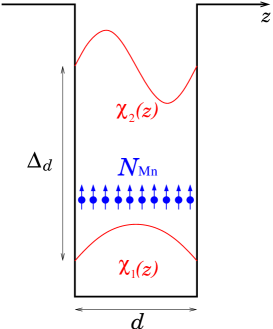
Figure 2: Sketch of a DMS quantum well. Itinerant carriers move freely in the $x$-$y$ plane, occupying subbands $\chi_{n}(z)$ due to quantum confinement along the $z$-axis (intersubband energy-gap $\Delta_{d}$). The magnetic-ion doping profile is represented by a continuous Mn-density distribution $N_{\rm Mn}(z)$.

The total Hamiltonian $H$ consist of four terms: $H=H_{\rm kin}+H_{\rm Z}+H_{\rm ex}+H_{\rm D}$. In the presence of a magnetic field ${\bf B}=\nabla\times{\bf A}$, the kinetic term for carriers of charge $e$ reads

$$H_{\rm kin} = \int{\rm d}^{2}r\int_{0}^{d}{\rm d}z\times$$

$$\hat{\Psi}^{\dagger}({\bf r},z)\left[\frac{-\hbar^{2}}{2m^{*}}\tilde{\nabla}^{2}+V(z)-\mu\right]\hat{\Psi}({\bf r},z)$$

$$= \int{\rm d}^{2}r\sum_{m=1}^{M}\sum_{\sigma}\hat{\psi}_{\sigma,m}^{\dagger}({\bf r})\left[\frac{-\hbar^{2}}{2m^{*}}\tilde{\nabla}_{\bf r}^{2}-\mu_{m}^{\prime}\right]\hat{\psi}_{\sigma,m}({\bf r}),$$

where $\tilde{\nabla}_{({\bf r})}=\nabla_{({\bf r})}-(ie/\hbar c){\bf A}$, $V(z)$ is the quantum-well confining potential, and $\mu^{\prime}_{m}=\mu-\epsilon_{m}$ is the effective subband-dependent chemical potential of the quasi-2D carrier gas, with $\epsilon_{m}$ the subband quantization energy. Here, we assumed a parabolic dispersion for the free carriers, with an effective mass $m^{*}$. This is well justified for n-doped systems, which have s-band conduction electrons. For hole doped systems, which have p-band valence carriers, this approximation is often useful for qualitative discussions. The Zeeman term is

$$H_{\rm Z}=\mu_{\rm B}{\bf B}\cdot\int{\rm d}^{2}r\int_{0}^{d}{\rm d}z\left[g_{e}\hat{\bf s}({\bf r},z)+g_{\rm Mn}{\bf S}({\bf r},z)\right],$$ (2)

where $\mu_{\rm B}>0$ is the Bohr magneton,

$$\hat{\bf s}({\bf r},z) = \frac{1}{2}\hat{\Psi}^{\dagger}({\bf r},z)~{}\boldsymbol{\tau}~{}\hat{\Psi}({\bf r},z)$$

$$= \sum_{m,m^{\prime}}\sum_{\sigma,\sigma^{\prime}}\chi_{m}(z)\chi_{m^{\prime}}(z)~{}\hat{\psi}_{\sigma,m}^{\dagger}({\bf r})\frac{\boldsymbol{\tau}_{\sigma\sigma^{\prime}}}{2}\hat{\psi}_{\sigma^{\prime},m^{\prime}}({\bf r})$$

is the quantum-well carrier spin density (with Pauli matrix vector $\boldsymbol{\tau}$), and ${\bf S}({\bf r},z)$ is the spin density of the Mn subsystem. The coupling between the carrier spins and the local Mn spins is described by

$$H_{\rm ex} = J_{\rm ex}\int{\rm d}^{2}r\int_{0}^{d}{\rm d}z~{}{\bf S}({\bf r},z)\cdot\hat{\bf s}({\bf r},z),$$ (4)

where $J_{\rm ex}<0$ corresponds to ferromagnetic and $J_{\rm ex}>0$ to antiferromagnetic coupling (i.e. to n- and p-doped host semiconductors, respectively). In symmetric quantum wells spin-orbit interactions are described by the Dresselhaus Hamiltoniannote9

$$H_{\rm D} = \gamma\int{\rm d}^{2}r\int_{0}^{d}{\rm d}z~{}\hat{\Psi}^{\dagger}({\bf r},z)~{}k_{z}^{2}\left(-\tau_{x}k_{x}+\tau_{y}k_{y}\right)\hat{\Psi}({\bf r},z)$$ (5)

$$= \gamma\int{\rm d}^{2}r\sum_{m,m^{\prime}=1}^{M}\sum_{\sigma,\sigma^{\prime}}~{}\langle k_{z}^{2}\rangle_{m,m^{\prime}}\times$$

$$\hat{\psi}_{\sigma,m}^{\dagger}({\bf r})\left(-\tau_{x}k_{x}+\tau_{y}k_{y}\right)_{\sigma\sigma^{\prime}}\hat{\psi}_{\sigma^{\prime},m^{\prime}}({\bf r}),$$

where $\langle k_{z}^{2}\rangle_{m,m^{\prime}}=\int_{0}^{d}{\rm d}z~{}\chi_{m}(z)~{}k_{z}^{2}~{}\chi_{m^{\prime}}(z)=\langle k_{m}^{2}\rangle\delta_{m,m^{\prime}}$ with $\langle k_{m}^{2}\rangle=(m\pi/d)^{2}$ when particle-in-a-box orbitals are used. The above spin-orbit Hamiltonian $H_{\rm D}$ leads to a $z$-oriented magnetic easy-axis as we have shown in earlier workKoenig and discuss later. For comments on spin-orbit coupling in the case of asymmetric quantum wells see Sec. III.5.

II.2 Effective action

In analogy to our earlier workKMd-bulk on bulk DMS ferromagnets, we want to describe elementary spin excitations in the DMS quantum well in a language where the itinerant-carrier degrees of freedom are integrated out. This leads to a retarded free-carrier mediated interaction between the Mn-ion $S=5/2$ spins. We are interested in small spin fluctuations about the mean-field magnetic state. The ground state of experimental doped quantum well DMS systems have sometimes been found to be ferromagnetic,Ohno-Science ; HWACTDd97 ; HTSNA97 ; HTSNSA98 ; OCMOADOO00 ; KFACTWdSGBSSWD00 ; BKBFCTWGD02 ; NST03 ; BBFCTWSKWGD03 ; MKBBFTCG03 ; WLLDFYWVM03 and sometimes exhibit complex spin-glass behavior. It is quite possible that the complex spin-glass states that sometimes occur are due to disorder effects that are not essential and can in principle be avoided, due for example to inhomogeneities in the Mn ion distribution, substitutional Mn ions, or other defects. In any event, the theory we discuss assumes a mean-field state in which all Mn ions are aligned. When this simple state is not the ground state of the system, or when we want to describe the collective excitations of a system that is above its ferromagnetic transition temperature, our theory will apply only in an external magnetic field that is strong enough to achieve substantial Mn ion spin polarization. We choose this field to be oriented in the $\hat{z}$ direction: ${\bf B}=(0,0,B)$. Because $g_{\rm Mn}>0$, the Mn spins then tend to align along the opposite direction. In the case of ferromagnets with anisotropy, we choose the $\hat{z}$ direction to be along an easy-axis.

It is convenient to represent the $S=5/2$ spins by Holstein-Primakoff (HP)HP40 bosons. For small fluctuations around the mean-field state the spin density ${\bf S}({\bf r},z)$ is approximated by $S^{+}\approx\bar{\omega}\sqrt{2N_{\rm Mn}(z)S}$, $S^{-}\approx\omega\sqrt{2N_{\rm Mn}(z)S}$, and $S^{z}=\bar{\omega}\omega-N_{\rm Mn}(z)S$, where the complex variables $\bar{\omega}$, $\omega$ are boson creation and annihilation operators that become bosonic coherent state labels in the path-integral formalism we employ. The vacuum with no HP bosons corresponds to full (negative) polarization of the Mn system, while the creation of a HP boson describes an increase in the total Mn spin by one unit. The partition function $Z$ of the compound system is calculated using a coherent-state path integral representation

$$Z=\int{\cal D}(\bar{\psi}\psi){\cal D}(\bar{\omega}\omega)~{}e^{-\int_{0}^{\beta}{\rm d}\tau~{}L(\bar{\psi}\psi,\bar{\omega}\omega)}$$ (6)

with ${\cal D}(\bar{\psi}\psi)\equiv{\cal D}(\bar{\psi}_{1}\psi_{1})\ldots{\cal D}(\bar{\psi}_{M}\psi_{M})$ and the Lagrangian

$$L(\bar{\psi}\psi,\bar{\omega}\omega) = \int{\rm d}^{2}r\left[\sum_{m=1}^{M}\bar{\psi}_{m}({\bf r,\tau})\partial_{\tau}\psi_{m}({\bf r,\tau})+\int_{0}^{d}{\rm d}z~{}\bar{\omega}({\bf r},z,\tau)\partial_{\tau}\omega({\bf r},z,\tau)\right]+H(\bar{\psi}\psi,\bar{\omega}\omega),$$ (7)

where the Grassmann numbers $\bar{\psi}=(\bar{\psi}_{1},\ldots,\bar{\psi}_{M})$ and $\psi=(\psi_{1},\ldots,\psi_{M})$ describe fermion (itinerant carrier) fluctuations within each of the $M$ subbands.

Since the Hamiltonian is bilinear in the fermionic fields, we can integrate them out and arrive at a representation for the bosonic partition function of the form $Z=\int{\cal D}(\bar{\omega}\omega)\exp(-S_{\rm eff}[\bar{\omega}\omega])$, with an effective action

$$S_{\rm eff}[\bar{\omega}\omega]=\int_{0}^{\beta}{\rm d}\tau\int{\rm d}^{2}r\int_{0}^{d}{\rm d}z~{}\left[\bar{\omega}({\bf r},z,\tau)\partial_{\tau}\omega({\bf r},z,\tau)+g_{\rm Mn}\mu_{\rm B}{\bf B}\cdot{\bf S}(\bar{\omega}\omega)\right]-\ln[\det G^{-1}(\bar{\omega}\omega)].$$ (8)

The total kernel $G^{-1}(\bar{\omega}\omega)$ can be split into a mean-field part, which does not depend on the bosonic (Mn spin excitation) fields $\bar{\omega}$ and $\omega$, and a fluctuating part by writing $G^{-1}(\bar{\omega}\omega)=G_{\rm MF}^{-1}+\delta G^{-1}(\bar{\omega}\omega)$, with

$$\left(G_{\rm MF}^{-1}\right)_{m,m^{\prime}} = \left[\partial_{\tau}-\frac{\hbar^{2}}{2m^{*}}\tilde{\nabla}_{\bf r}^{2}-\mu^{\prime}_{m}\right]\delta_{m,m^{\prime}}$$

$$+ \frac{1}{2}\left(g_{e}\mu_{\rm B}B\delta_{m,m^{\prime}}-\Delta_{m,m^{\prime}}\right)\tau_{z}$$

$$+ \gamma\langle k_{m}^{2}\rangle\left(-\tau_{x}k_{x}+\tau_{y}k_{y}\right)\delta_{m,m^{\prime}},$$

$$\delta G_{m,m^{\prime}}^{-1}(\bar{\omega}\omega) = \frac{J_{\rm ex}}{2}\int_{0}^{d}{\rm d}z~{}\chi_{m}(z)\chi_{m^{\prime}}(z)\times$$

$$\left[\sqrt{2N_{\rm Mn}(z)S}~{}(\bar{\omega}~{}\tau^{-}+\omega~{}\tau^{+})+\bar{\omega}\omega\tau_{z}\right].$$

The exchange coupling contributes to the conduction band spin-splitting in $G_{\rm MF}$ through the mean-field interaction $\Delta_{m,m^{\prime}}=J_{\rm ex}(\bar{N}_{\rm Mn})_{m,m^{\prime}}S$, where $(\bar{N}_{\rm Mn})_{m,m^{\prime}}=\int_{0}^{d}{\rm d}z~{}\chi_{m}(z)\chi_{m^{\prime}}(z)N_{\rm Mn}(z)$.note1 We recognize here that coupling to a Mn-spin system with an inhomogeneous doping profile $N_{\rm Mn}(z)$ leads to mixing of the quantum-well subbands. These intersubband interactions are present at the mean-field level, as seen in Eq. (II.2), but also appear in the term which expresses the coupling between carriers and local moment fluctuations, Eq. (II.2).

II.3 Quantum-well subband decoupling and independent spin-wave theory

The above picture simplifies considerably when quantum-well subband mixing is negligible,LeePRB i.e. when the energy gap $\Delta_{d}$ (see Fig. 2) is much larger than the spin-splitting energies $\Delta_{m,m^{\prime}}$. This regime can be reached either by narrowing the quantum well ($\Delta_{d}\rightarrow\infty$), or by diluting the Mn doping ($\Delta_{m,m^{\prime}}\rightarrow 0$), independently of the number of occupied subbands $M$, which is controlled by the carrier density. In this limit we arrive at a Green’s function that is diagonal in subband space, with $G^{-1}_{m}=(G_{\rm MF}^{-1})_{m}+\delta G^{-1}_{m}$,

$$(G_{\rm MF}^{-1})_{m} = \left[\partial_{\tau}-\frac{\hbar^{2}}{2m^{*}}\tilde{\nabla}_{\bf r}^{2}-\mu^{\prime}_{m}\right]$$

$$+ \frac{1}{2}(g_{e}\mu_{\rm B}B-\Delta_{m})\tau_{z}$$

$$+ \gamma\langle k_{m}^{2}\rangle\left(-\tau_{x}k_{x}+\tau_{y}k_{y}\right),$$

$$\delta G^{-1}_{m}(\bar{\omega}\omega) = \frac{J_{\rm ex}}{2}\int_{0}^{d}{\rm d}z~{}\chi^{2}_{m}(z)\times$$

$$\left[\sqrt{2N_{\rm Mn}(z)S}~{}(\bar{\omega}~{}\tau^{-}+\omega~{}\tau^{+})+\bar{\omega}\omega\tau_{z}\right].$$

Here $\Delta_{m}=\Delta_{m,m}$ is the subband-dependent exchange contribution to the itinerant carrier mean-field splitting. This approximation leads to a convenient subband separation $\ln[\det G^{-1}]=\sum_{m=1}^{M}\ln[\det G^{-1}_{m}]$ in Eq. (8).

Expanding $\ln[\det G^{-1}_{m}]$ up to second order in $\delta G^{-1}_{m}$, $\ln[\det G^{-1}_{m}]={\rm tr}[\ln(G_{\rm MF}^{-1})_{m}]+{\rm tr}[(G_{\rm MF})_{m}\delta G^{-1}_{m}]-(1/2){\rm tr}[(G_{\rm MF})_{m}\delta G^{-1}_{m}(G_{\rm MF})_{m}\delta G^{-1}_{m}]+\ldots$, and collecting all contributions up to quadratic order in $\bar{\omega}$ and $\omega$ we arrive at an independent spin-wave theory where the spin excitations are treated as non-interacting HP bosons. This is a good approximation for temperatures well below the maximum of the ferromagnetic transition temperature and/or the temperature defined by Zeeman coupling to the external field, in which case spin excitation amplitudes are small. Fourier transforming the resulting spin-wave action (keeping $z$ in real space and defining bosonic Matsubara frequencies $\nu_{n}$) we obtain

$$S_{\rm eff}[\bar{\omega}\omega] = \frac{1}{\beta}\sum_{n}\int\frac{{\rm d}^{2}k}{(2\pi)^{2}}\int\frac{{\rm d}^{2}k^{\prime}}{(2\pi)^{2}}\int_{0}^{d}{\rm d}z\int_{0}^{d}{\rm d}z^{\prime}~{}\times$$ (13)

$$\bar{\omega}({\bf k},z,\nu_{n})D^{-1}({\bf k},{\bf k^{\prime}},z,z^{\prime},\nu_{n})\omega({\bf k^{\prime}},z^{\prime},\nu_{n}).~{}~{}~{}~{}~{}$$

The kernel of the quadratic action (13) is the inverse of the spin-wave propagator $D({\bf k},{\bf k^{\prime}},z,z^{\prime},\nu_{n})$ and is given by

$$D^{-1}({\bf k},{\bf k^{\prime}},z,z^{\prime},\nu_{n}) = \left[-i\nu_{n}+g_{\rm Mn}\mu_{B}B-\frac{J_{\rm ex}}{2}\sum_{m=1}^{M}(n^{\downarrow}_{m}-n^{\uparrow}_{m})\chi_{m}^{2}(z)\right]\delta(z-z^{\prime})\delta({\bf k}-{\bf k^{\prime}})$$ (14)

$$+ \frac{J_{\rm ex}^{2}}{2}S~{}\sqrt{N_{\rm Mn}(z)N_{\rm Mn}(z^{\prime})}~{}\sum_{m=1}^{M}\chi_{m}^{2}(z)\chi_{m}^{2}(z^{\prime})\sum_{\alpha,\alpha^{\prime}}~{}\frac{f(\epsilon_{m,\alpha}^{\downarrow})-f(\epsilon_{m,\alpha^{\prime}}^{\uparrow})}{i\nu_{n}+\epsilon_{m,\alpha}^{\downarrow}-\epsilon_{m,\alpha^{\prime}}^{\uparrow}}~{}\Phi_{m}^{\alpha,\alpha^{\prime}*}({\bf k})~{}\Phi_{m}^{\alpha,\alpha^{\prime}}({\bf k^{\prime}}).$$

We arrive at Eq. (14) by introducing a wave-function representation of the mean-field Green’s function of Eq. (II.3)

$$(G_{\rm MF})_{m}^{\sigma}({\bf r^{\prime}},{\bf r},\nu_{n})=\sum_{\alpha}\frac{\phi_{m,\alpha}^{\sigma}({\bf r^{\prime}})\phi_{m,\alpha}^{\sigma*}({\bf r})}{i\nu_{n}-\epsilon_{m,\alpha}^{\sigma}},$$ (15)

where $\phi_{m,\alpha}^{\sigma}({\bf r})$ are the 2D mean-field itinerant carrier eigenstates for spin $\sigma$ and subband $m$, with energy $\epsilon_{m,\alpha}^{\sigma}=\epsilon_{\alpha}+(\sigma/2)(g_{e}\mu_{\rm B}B-\Delta_{m})\sqrt{1+4\epsilon^{{\rm so}}_{m,\alpha}/(g_{e}\mu_{\rm B}B-\Delta_{m})}-\mu^{\prime}_{m}$. sakurai The index $\alpha$ accounts for quantum-numbers associated with orbital motion, with kinetic and spin-orbit energies $\epsilon_{\alpha}$ and $\epsilon^{{\rm so}}_{m,\alpha}=|\langle\downarrow,m,\alpha|\gamma k_{z}^{2}(-\tau_{x}k_{x}+\tau_{y}k_{y})|\uparrow,m,\alpha\rangle|^{2}/(g_{e}\mu_{\rm B}B-\Delta_{m})$, respectively. To first order in spin-orbit coupling ($\epsilon^{{\rm so}}_{m,\alpha}\ll(g_{e}\mu_{\rm B}B-\Delta_{m})$), the eigenenergy is $\epsilon_{m,\alpha}^{\sigma}=\epsilon_{\alpha}+(\sigma/2)(g_{e}\mu_{\rm B}B-\Delta_{m})+\sigma\epsilon^{{\rm so}}_{m,\alpha}-\mu^{\prime}_{m}$. In Eq. (14) $f(\epsilon)$ is the Fermi distribution, $n^{\sigma}_{m}$ is the 2D mean-field itinerant carrier spin density for the $m$,$\sigma$ subband obtained by summing over occupied states, and we have introduced Fourier-transform factors defined by

$$\Phi_{m}^{\alpha,\alpha^{\prime}}({\bf k})=\int{\rm d}^{2}r~{}\exp(i{\bf k}\cdot{\bf r})~{}\phi_{m,\alpha}^{\uparrow}({\bf r})\phi_{m,\alpha^{\prime}}^{\downarrow*}({\bf r}).$$ (16)

The first line on the r.h.s. of Eq. (14) is local in space. It represents the mean-field expression for the exchange field that the Mn spins experience. The second line is nonlocal in space and describes correlation effects that occur because of the (space- and $m$-subband-dependent) response of the quantum-well carriers to Mn spin orientations. We note that $D^{-1}$ is not a function of $z-z^{\prime}$ only, because of the absence of translational symmetry in the $z$-direction. Additionally, a 2D Debye cutoff $k_{\rm D}^{2}=4\pi N_{\rm Mn}/(N/d)$ ensures that our continuum approximation has the correct number of magnetic-impurity degrees of freedom. [Here, $N_{\rm Mn}=\int_{0}^{d}{\rm d}zN_{\rm Mn}(z)/d$  note3 and $N$ is the number of growth-direction modes included in the theory as we explain below. We associate $N$ with the mean number of Mn ions encountered on crossing the quantum well; e.g. for isotropic doping $N\sim N_{\rm Mn}^{1/3}d$.]

We comment now on the factors $\Phi_{m}^{\alpha,\alpha^{\prime}}({\bf k})$ which are trivial for the plane-wave functions of field-free systems. They are included to allow us to simply account for the consequences of orbital coupling of itinerant carriers to magnetic fields. The index $\alpha$ includes both the Landau levels index and the gauge-dependent index for states within a Landau level. At zero field the mean-field eigenstates $\phi_{m,\alpha}^{\sigma}({\bf r})$ are plane waves with momentum $\alpha\equiv{\bf q}$, kinetic energy $\epsilon_{\bf q}=\hbar^{2}q^{2}/(2m^{*})$ and spin-orbit energy $\epsilon^{\rm so}_{m,{\bf q}}=\gamma^{2}\langle k^{2}_{m}\rangle^{2}q^{2}/(g_{e}\mu_{\rm B}B-\Delta_{m})$. In either case Eq. (14) is diagonal in the in-plane momentum ${\bf k}$ and we denote its diagonal elements by $D^{-1}({\bf k},z,z^{\prime},i\nu_{n})$. The case of a uniform magnetic field was considered in Ref. Koenig, and will not be discussed further in this paper.

III Elementary spin excitations

Even the bulk-like epitaxially grown thin film samples studied in typical experiments do not contain a very large number of occupied 2D carrier subbands. Our formalism could in principle be used to calculate the collective modes of thin films, taking account of the variation in Mn density across the film, although the approach becomes numerically cumbersome when more than a few subbands are occupied. It is likely, though, that greater insight into vertical inhomogeneity effects in thin-films can be obtained with more approximate approaches.RRLZFJ03 We limit the discussion here to true quantum-well samples in which a single subband is occupied ($M=1$) and subband mixing can be neglected. For definiteness we concentrate on the case of constant Mn density $N_{\rm Mn}(z)=N_{\rm Mn}$. Similarly we assume that the state we are studying is an ordered ferromagnetic phase with the $\hat{z}$-direction magnetic easy-axis that is favored by (weak) spin-orbit coupling. The situation in which the magnetization direction has been reoriented by an external magnetic field is readily included in the formalism as explained above. Generalizations to the cases of multiple subbands, and inhomogeneous Mn density are straightforward.

Collective spin excitation dispersion $\Omega({\bf k})$ branches are located by finding the frequencies at which the determinant, $\det[D^{-1}({\bf k},z,z^{\prime},i\nu_{n}=\Omega)]$, of the quadratic action kernel in Eq. (13) vanishes. The continuum of spin-flip particle-hole (Stoner) excitations is located by identifying the ${\bf k}$-dependent frequency range over which ${\rm Im}[D^{-1}({\bf k},z,z^{\prime},i\nu_{n})]$ is non-zero after the analytic continuation $i\nu_{n}\rightarrow\Omega+i0^{+}$.

III.1 Stoner continuum

We start by evaluating the continuum of Stoner excitations introduced above. They correspond to flipping a single spin in the itinerant carrier subsystem and typically have relatively large energies of the order of the itinerant carrier mean-field spin splitting $\Delta=J_{\rm ex}N_{\rm Mn}S$. The continuum is obtained by determining the conditions for ${\rm Im}[D^{-1}({\bf k},z,z^{\prime},\Omega+i0^{+})]\neq 0$. With this aim it is convenient to define the dimensionless carrier spin-polarization $p=(n^{\uparrow}-n^{\downarrow})/(n^{\uparrow}+n^{\downarrow})$ and the Fermi energy of the majority-spin carrier band $\epsilon_{\rm s}=\mu^{\prime}+|\Delta|/2$, where $\mu^{\prime}$ is the effective chemical potential of the 2D carrier gas. For half-metallic carriers ($|p|=1$, $\epsilon_{\rm s}\leq|\Delta|$, see Appendix A) these excitations carry spin $S_{z}=\pm 1$, depending on the sign of $\Delta$ (i.e. on whether the coupling between carriers and Mn ions is ferromagnetic or antiferromagnetic). On the other hand, for partly polarized carriers ($|p|<1$, $\epsilon_{\rm s}>|\Delta|$, see Appendix A) excitations carrying both $S_{z}=1$ and $S_{z}=-1$ contribute, independent of the sign of $\Delta$. In the absence of spin-orbit coupling ($\gamma=0$), one finds a continuum of excitations with dispersion lying between the curves $-\Delta-{\rm sign}[\Delta]\epsilon_{\bf k}\pm 2\sqrt{\epsilon_{\rm s}\epsilon_{\bf k}}$ for $\epsilon_{\rm s}\leq|\Delta|$, and also between $-\Delta+{\rm sign}[\Delta]\epsilon_{\bf k}\pm 2\sqrt{(\epsilon_{\rm s}-|\Delta|)\epsilon_{\bf k}}$ for $\epsilon_{\rm s}>|\Delta|$. For small spin-orbit coupling, the energy width of the Stoner continuum does not vanish at ${\bf k}=0$, instead approaching the width

$$\Delta\Omega=4\frac{\gamma^{2}\langle k_{z}^{2}\rangle^{2}m^{*}\epsilon_{\rm s}}{\hbar^{2}|\Delta|}.$$ (17)

In the case of multi-subband quantum wells ($M>1$) multiple continua arise, each of them associated with the corresponding subband by means of $\Delta_{m}$, $\langle k_{m}^{2}\rangle$ and $\mu^{\prime}_{m}$.

III.2 Spin-wave modes

The number of collective modes that appear in our theory depends on the doping concentration and the width of the quantum well. It is natural to choose the mean number $N$ of Mn ions along the $z$-direction as a dimensional cutoff for the representation of the inverse propagator $D^{-1}({\bf k},z,z^{\prime},\Omega)$. This motivates the choice of an appropriate basis of $N$ orthonormal excitation profiles $\{\omega_{n}(z)\}$, with $0\leq n\leq N-1$ and $\int_{0}^{d}{\rm d}z~{}\omega_{n}(z)\omega_{n^{\prime}}(z)=\delta_{nn^{\prime}}$, for expanding Eq. (14), i.e.,

$$D^{-1}_{nn^{\prime}}({\bf k},\Omega)=\int\limits_{0}^{d}{\rm d}z\int\limits_{0}^{d}{\rm d}z^{\prime}\omega_{n}(z)D^{-1}({\bf k},z,z^{\prime},\Omega)\omega_{n^{\prime}}(z^{\prime}).\,\,$$ (18)

We later solve $\det[D^{-1}_{nn^{\prime}}({\bf k},\Omega)]_{N\times N}=0$ for $\Omega$ and obtain a set of $N+1$ solutions $\{\Omega_{(l)}({\bf k})\}$ with the mode profiles $\omega_{(l)}(z)=\sum_{n}c^{(l)}_{n}\omega_{n}(z)$. The coefficients ${\bf c}^{(l)}=(c^{(l)}_{0},c^{(l)}_{1},\ldots,c^{(l)}_{N-1})$ are obtained from $[D^{-1}_{nn^{\prime}}({\bf k},\Omega_{(l)})]_{N\times N}{\bf c}^{(l)}=0$. We combine this procedure with a Debye cut-off of the 2D wavevectors to get the correct number of magnetic degrees of freedom. This approximate procedure, a silent partner of the continuum Mn density approximation that we use to avoid dealing with disorder, obviously breaks down to some degree for the shortest wavelength modes which must be sensitive to the discreteness of the magnetic degrees of freedom. The procedure should be accurate for longer wavelength modes, however, and we believe that it gives a good qualitative description of the overall spectrum. We employ it without further comment in the rest of the paper.

We assume that the magnetization direction of the Mn spins located at the borders of the quantum well is not fixed by an anisotropy field or magnetic coupling to an adjacent layer. Then we can use free-end boundary conditions for the magnetic excitations, ${\rm d}\omega_{n}(z)/{\rm d}z=0$ at $z=0,d$. This determines the choice of the basis functions

$$\omega_{n}(z)=a_{n}\cos\left(\frac{n\pi z}{d}\right),~{}~{}~{}a_{n}=\left\{\begin{array}[]{cc}\sqrt{1/d}&{\rm for}~{}n=0\\ \sqrt{2/d}&{\rm for}~{}n\geq 1\end{array}\right..$$ (21)

We now calculate the matrix elements $D^{-1}_{nn^{\prime}}({\bf k},\Omega)$ using Eqs. (14)-(21) for $M=1$ and constant $N_{\rm Mn}$ in the absence of an external magnetic field. The quantum-well subband is defined by the wave function $\chi(z)=\sqrt{2/d}~{}\sin(\pi z/d)$. We find

$$D^{-1}_{nn^{\prime}}({\bf k},\Omega)=-\Omega\delta_{nn^{\prime}}+x_{\rm s}|\Delta|\left[M_{1}+I({\bf k},\Omega)M_{2}\right]_{nn^{\prime}},$$ (22)

with the $N\times N$-matrices

$$M_{1} = \left(\begin{array}[]{cccccc}1&0&-1/\sqrt{2}&0&0&\ldots\\ 0&1/2&0&-1/2&0&\ldots\\ -1/\sqrt{2}&0&1&0&-1/2&\ldots\\ 0&-1/2&0&1&0&\ldots\\ 0&0&-1/2&0&1&\ldots\\ \vdots&\vdots&\vdots&\vdots&\vdots&\ddots\end{array}\right)_{N\times N}$$ (29)

$$M_{2} = \left(\begin{array}[]{ccccc}1&0&-1/\sqrt{2}&0&\ldots\\ 0&0&0&0&\ldots\\ -1/\sqrt{2}&0&1/2&0&\ldots\\ 0&0&0&0&\ldots\\ \vdots&\vdots&\vdots&\vdots&\ddots\end{array}\right)_{N\times N}.$$ (35)

In Eq. (22) we have defined the ratio of the free-carrier spin-density to the Mn spin density $x_{\rm s}=|n^{\uparrow}-n^{\downarrow}|/(2N_{\rm Mn}Sd)$, which typically satisfies $x_{\rm s}\ll 1$, and the dimensionless integral

$$I({\bf k},\Omega)=\frac{|\Delta|}{|n^{\uparrow}-n^{\downarrow}|}\int\frac{{\rm d}^{2}q}{(2\pi)^{2}}~{}\frac{f(\epsilon_{\bf q}^{\downarrow})-f(\epsilon_{{\bf q}+{\bf k}}^{\uparrow})}{\Omega+\epsilon_{\bf q}^{\downarrow}-\epsilon_{{\bf q}+{\bf k}}^{\uparrow}}.$$ (36)

The last can be evaluated analytically for $T=0$ in the absence of spin-orbit coupling, as described briefly in Appendices A and B.

The term containing $M_{1}$ corresponds to the term proportional to $J_{\rm ex}$ in Eq. (14) and describes the mean-field exchange interaction between Mn spins with free-carrier spins. The appearance of off-diagonal matrix elements, indicating a mixing of basis functions for the Mn spin excitations, is of geometric origin, determined by the projection $\int_{0}^{d}{\rm d}z~{}\chi^{2}(z)\omega_{n}(z)\omega_{n^{\prime}}(z)$. The nonlocal correlations are accounted for by the term containing $M_{2}$, which corresponds to the term proportional to $J_{\rm ex}^{2}$ in Eq. (14). Mixing appears here also, determined this time by $[\int_{0}^{d}{\rm d}z~{}\chi^{2}(z)\omega_{n}(z)][\int_{0}^{d}{\rm d}z~{}\chi^{2}(z)\omega_{n^{\prime}}(z)]$. The structure of the matrices in Eqs. (29) and (35) shows that basis functions with different parity $\{\omega_{n}(z)\}$ do not mix.note4 This allows us to write the expanded kernel (22) as the (external) product of two matrices corresponding to even ($+$) and odd ($-$) modes: $[D^{-1}_{nn^{\prime}}({\bf k},\Omega)]_{N\times N}=[D^{-1}_{nn^{\prime}}({\bf k},\Omega)]^{+}_{N^{+}\times N^{+}}\otimes[D^{-1}_{nn^{\prime}}({\bf k},\Omega)]^{-}_{N^{-}\times N^{-}}$, with $N^{+}+N^{-}=N$. Spin modes obtained as solutions of $\det[D^{-1}_{nn^{\prime}}({\bf k},\Omega)]_{N\times N}=0$ can now be classified according to their parity by solving separately $\det[D^{-1}_{nn^{\prime}}({\bf k},\Omega)]^{+}_{N^{+}\times N^{+}}=0$ and $\det[D^{-1}_{nn^{\prime}}({\bf k},\Omega)]^{-}_{N^{-}\times N^{-}}=0$, respectively. This leads to $N^{+}+1$ even modes and $N^{-}$ odd ones. Moreover, it is possible to see from Eq. (22) that $[D^{-1}_{nn^{\prime}}({\bf k},\Omega)]^{-}_{N^{-}\times N^{-}}$ is independent of $I({\bf k},\Omega)$. This means that correlations between local moment and band configurations do not influence spin modes of odd parity. As a consequence these modes are dispersionless, note4 as we see explicitly below. More interesting are the even modes for which correlation effects due to the coupling to itinerant carriers show up.

In the following we apply the above formulation to the cases of dilute and moderate Mn doping in the limit of vanishing spin-orbit coupling ($\gamma\rightarrow 0$). We then (Sec. III.5) comment on how these results are altered by a finite $\gamma$.

III.3 Dilute Mn doping

For illustration we start discussing the limiting case of dilute Mn doping or, equivalently, narrow quantum wells. This corresponds to very few Mn ions across the quantum well leading in our approach to a low-dimensional kernel $[D^{-1}_{nn^{\prime}}({\bf k},\Omega)]_{N\times N}$ (Eq. (22)) with $N$ of order one. In this situation we can easily approach the problem analytically. We choose for simplicity $N^{+}=N^{-}=1$ (i.e. $N=2$). In this case the dispersion relations of even and odd spin modes (corresponding to $\omega_{0}(z)$ and $\omega_{1}(z)$, respectively; see Eq. (21)) are obtained by solving

$$\det[D^{-1}_{nn^{\prime}}({\bf k},\Omega)]^{+} = [1+I({\bf k},\Omega)]x_{\rm s}|\Delta|-\Omega=0,$$ (37)

$$\det[D^{-1}_{nn^{\prime}}({\bf k},\Omega)]^{-} = x_{\rm s}|\Delta|/2-\Omega=0\,.$$ (38)

Eq. (38) leads to a single odd mode with flat dispersion $\Omega^{-}=x_{\rm s}|\Delta|/2$. For the calculation of the even modes we limit ourselves for now to the case of ferromagnetic coupling ($\Delta<0$) at $T=0$; the difference between ferromagnetic and antiferromagnetic cases is commented on later in Sec. IV. We solve Eq. (37) for long and short wavelengths (i.e. long and short range correlations), using the expansions (48) and (49) up to first order in $\epsilon_{\bf k}$ and $1/\epsilon_{\bf k}$, respectively. This leads to two solutions: one soft mode $\Omega^{+}_{\rm soft}<x_{\rm s}|\Delta|$, and one hard mode $\Omega^{+}_{\rm stiff}\sim|\Delta|$, where typically $\Omega^{+}_{\rm soft}\ll\Omega^{+}_{\rm stiff}$. For half-metallic carriers ($|p|=1$, $\epsilon_{\rm s}\leq|\Delta|$, see Appendix A) we obtain for the small-and large-momentum limit

$$\Omega^{+}_{\rm soft}({\bf k}) = \frac{x_{\rm s}}{1+x_{\rm s}}\left(1-\frac{\epsilon_{\rm s}}{|\Delta|}\right)\epsilon_{\bf k}+O(\epsilon_{\bf k}^{2})$$ (39)

$$= x_{\rm s}|\Delta|\left(1-\frac{|\Delta|}{\epsilon_{\bf k}}\right)+O(1/\epsilon_{\bf k}^{2}),$$ (40)

$$\Omega^{+}_{\rm stiff}({\bf k}) = (1+x_{\rm s})|\Delta|+\frac{1}{1+x_{\rm s}}\left(1+\frac{\epsilon_{\rm s}}{x_{\rm s}|\Delta|}\right)\epsilon_{\bf k}+O(\epsilon_{\bf k}^{2}),$$

respectively. Correspondingly, for partly polarized carriers ($|p|<1$, $\epsilon_{\rm s}>|\Delta|$, using the results summarized in Appendix A) we find

$$\Omega^{+}_{\rm soft}({\bf k}) = 0+O(\epsilon_{\bf k}^{2})$$ (42)

$$= x_{\rm s}|\Delta|\left(1+\left(1-\frac{2\epsilon_{\rm s}}{|\Delta|}\right)\frac{|\Delta|}{\epsilon_{\bf k}}\right)+O(1/\epsilon_{\bf k}^{2}),$$ (43)

$$\Omega^{+}_{\rm stiff}({\bf k}) = (1+x_{\rm s})|\Delta|+\frac{1}{x_{\rm s}}\left(\frac{2\epsilon_{\rm s}}{|\Delta|}-1\right)\epsilon_{\bf k}+O(\epsilon_{\bf k}^{2}),$$ (44)

for small and large momenta, respectively.

The branch $\Omega^{+}_{\rm soft}$ corresponds to a gapless Goldstone-mode reflecting the spontaneous breaking of rotational symmetry for the Mn spins subsystem, as expected generically in ferromagnets and found in bulk magnetic semiconductors. KMd-bulk At long wavelengths ($\epsilon_{\bf k}\rightarrow 0$) the dispersion in bulk isotropic ferromagnets is proportional to the spin stiffness $\rho$ divided by the magnetization ${\cal M}$ (i.e. $\Omega=(\rho/{\cal M})k^{2}$). Similarly, in the adiabatic limit $\epsilon_{\rm s}\ll|\Delta|$, our long wavelength result for quantum wells (39) shows a spin stiffness due only to the increase in kinetic energy of the fully spin-polarized band when the spin orientation is spatial dependent, $\rho=\hbar^{2}n^{\downarrow}/(4m^{*})$. The magnetization, with parallel contributions from Mn ions and itinerant carriers coupled ferromagnetically, reads ${\cal M}=SN_{\rm Mn}d+n^{\downarrow}/2=SN_{\rm Mn}d(1+x_{\rm s})$. However, unlike bulk systems the spin stiffness vanishes as $\epsilon_{\rm s}\rightarrow|\Delta|$, Eq. (39), and stays equal to zero for $\epsilon_{\rm s}>|\Delta|$, Eq. (42). This unusual feature should lead to some non-standard phenomenology in these ferromagnets, for example in the physics that controls domain wall widths and finite-temperature magnetization suppression. For short wavelengths ($\epsilon_{\bf k}\rightarrow\infty$), Eqs. (40) and (43), the excitation energy $\Omega^{+}_{\rm soft}$ tends to a mean-field value $x_{\rm s}|\Delta|$, corresponding to the magnetic-ion spin splitting.

The branch of stiff excitations $\Omega^{+}_{\rm stiff}$, Eqs. (LABEL:opem1dtp) and (44), is primarily band-like in character and is centered around the much larger energy scale of the itinerant carrier mean-field spin splitting $|\Delta|$.

III.4 Moderate Mn doping

We now switch to the case of higher dimensions ($N^{+},N^{-}>1$), which corresponds to several Mn ions across the quantum well. As in the previous Sec. III.3 dedicated to dilute Mn doping, we consider Mn spins coupled ferromagnetically to the itinerant carriers ($\Delta<0$) at $T=0$. Comments regarding the antiferromagnetic coupling case will be introduced later in Sec. IV. As an example we choose $N^{+}=N^{-}=5$ with a relative spin density $x_{\rm s}=0.05$. The dispersions corresponding to even and odd modes are obtained numerically by solving $\det[D^{-1}_{nn^{\prime}}({\bf k},\Omega)]^{+}_{5\times 5}=0$ and $\det[D^{-1}_{nn^{\prime}}({\bf k},\Omega)]^{-}_{5\times 5}=0$, respectively. This leads to a set of six even modes, five relatively soft ($\Omega^{+}_{(l)}$) and one hard ($\Omega^{+}_{\rm stiff}$), and five odd modes ($\Omega_{(l)}^{-}$). The index $l$ ($1\leq l\leq 5$) orders the modes from the bottom ($l=1$) to the top ($l=5$) of the spectrum in each case. Our results for $\Omega^{+}_{(l)}$ (solid lines) and $\Omega_{(l)}^{-}$ (dashed lines) are summarized in Fig. 3(a)-(c) for three characteristic ratios $\epsilon_{\rm s}/|\Delta|=$ 0.9, 0.975, and 1.5, respectively. Panels (a) and (b) correspond to half-metallic carriers while panel (c) depicts results for the case of partly polarized carriers. Related results for $\Omega^{+}_{\rm stiff}$ are shown in Fig. 4. In all plots the shaded zones represents the Stoner continuum. For each case, the normalized excitation energies $\Omega/|\Delta|$ are plotted as a function of the normalized $k$-vector $\sqrt{\epsilon_{\bf k}/|\Delta|}=A(k/k_{\rm D})$, where $A=\sqrt{\epsilon_{{\bf k}_{\rm D}}/|\Delta|}$. For typical DMS quantum well systems we estimate that $A>10$. Hence, the results shown in Figs. 3 and 4 correspond to $k/k_{\rm D}\ll 1$, the regime well below the Debye cut-off in which the continuum approximation is most reliable.

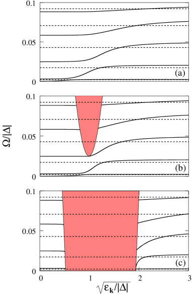
Figure 3: Dispersion of low-energy spin excitations in a single-subband DMS quantum well with ferromagnetic coupling ($\Delta<0$) and dimensional cut-off $N^{+}=N^{-}=5$ (see text). Panels (a) and (b) correspond to half-metallic (i.e. fully polarized) carriers ($\epsilon_{\rm s}/|\Delta|=0.9$ and 0.975, respectively). Panel (c) depicts results for partly polarized carriers ($\epsilon_{\rm s}/|\Delta|=1.5$). The even modes $\Omega^{+}_{(l)}$ are denoted by solid lines and the dispersionless odd modes $\Omega_{(l)}^{-}$ by dashed lines. The spatial profiles of the even and odd modes are illustrated in Fig. 5(a)-(e) and Fig. 7, respectively. The integer labels order the modes by increasing frequency. The shaded zones indicate the Stoner continuum.

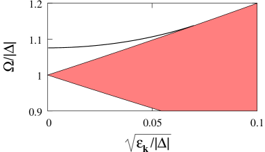
Figure 4: Dispersion of high-energy spin excitations in a single-subband DMS quantum well with ferromagnetic coupling ($\Delta<0$) and dimensional cut-off $N^{+}=5$ (see text) for half-metallic (i.e. fully polarized) carriers with $\epsilon_{\rm s}/|\Delta|=0.9$. Similar features appear for partly polarized carriers ($\epsilon_{\rm s}/|\Delta|>1$). The stiff branch $\Omega^{+}_{\rm stiff}$ (solid lines) corresponds to the mode $\omega^{+}_{\rm stiff}$ (Fig. 5(f)). The Stoner continuum is represented by the shaded zone. Ferromagnetic interactions with the local moments peel a collective mode off the particle-hole continuum.

We start by discussing the properties of the relatively soft even modes $\Omega^{+}_{(l)}$ depicted in Fig. 3 by solid lines. Panel (a) corresponding to $\epsilon_{\rm s}/|\Delta|=$ 0.9 is representative of results for half-metallic cases with $\epsilon_{\rm s}/|\Delta|\ll 1$. There we find a set of modes at ${\bf k}=0$ that are distributed in the small energy window $0\leq\Omega<2x_{\rm s}|\Delta|$ and have $k^{2}$ dispersion at finite wavevectors, corresponding to a finite spin-stiffness. The upper limit in this spectrum is twice the mean-field value predicted in the case of bulk systems. KMd-bulk This is due to the fact that the carrier spin density is modulated by $\chi(z)=\sqrt{2/d}\sin(\pi z/d)$ across the quantum well (lower density close to the border $z=0,d$ and higher density close to the center $z=d/2$). Spin modes with large relative amplitude near the center of the quantum well see a carrier spin density which is effectively higher than in the uniform spin-density bulk case.

The first branch $\Omega^{+}_{(1)}$ corresponds to a gapless Goldstone-mode $\omega^{+}_{(1)}(z)=\omega_{0}(z)$, Fig. 5(a), similar to the one discussed above for the dilute Mn doping case, in Sec. III.3. For the $l>1$ modes, the spatial structure $\omega^{+}_{(l)}(z)$ is not constant within the quantum well (see Figs. 5(b)-(e)) and the energies $\Omega^{+}_{(l)}({\bf k})$ therefore approach a finite value as $|{\bf k}|\to 0$. The dependence of the excitation energies $\Omega^{+}_{(l)}({\bf k}=0)$ on $l$ is not obvious, since the gap is not simply related to the effective transverse momentum $k_{z}^{+(l)}=\int_{0}^{d}{\rm d}z~{}\omega^{+}_{(l)}\partial\omega^{+}_{(l)}/\partial z$ associated to each mode. Instead, the local excitation density $\omega^{+2}_{(l)}(z)$ and its correlation with the carrier density, proportional to $\chi^{2}(z)$, is more relevant. (See Fig. 5 for a comparison). We illustrate the $l$-dependence of $\Omega^{+}_{(l)}({\bf k}=0)$ in Fig. 6 for $N^{+}=20$ (full circles). We observe a spin-mode accumulation close to the boundaries of the spectrum that is not evident for small $N^{+}$. Furthermore, the inset in Fig. 6 shows that the dispersion does not appear to be quadratic for small $l$. Since $\Omega^{+}_{(1)}({\bf k}=0)=0$, a quadratic fit has a single free parameter. The dashed (dotted) line corresponds to a quadratic fit between the $l=1$-mode and the $l=2$- ($l=5$) one. The curves differ by a (relatively large) factor of order 3.5.

Figure 5: Spatial profiles across a single-subband DMS quantum well for even parity collective modes (solid lines). The well has width $d$ ($0\leq z/d\leq 1$), ferromagnetic coupling ($\Delta<0$), and the dimensional cut-off $N^{+}=5$ (see text). The carrier density $\chi^{2}(z)$ (dashed line) is shown for comparison. Note that the Goldstone mode, panel (a), is constant in space corresponding to uniform spin rotation. The other modes tend to have higher energy when they have higher weight toward the middle of the quantum well, where exchange interactions are stronger.

Figure 6: Dispersion of low-energy spin excitations in a single-subband DMS quantum well for in-plane momentum ${\bf k}=0$, ferromagnetic coupling ($\Delta<0$), and dimensional cut-off $N^{+}=N^{-}=20$, as a function of the mode index $l$ (see text). The full circles depict the excitation energies $\Omega^{+}_{(l)}({\bf k}=0)$ of even modes $\omega^{+}_{(l)}$, while the empty circles correspond to $\Omega^{-}_{(l)}({\bf k}=0)$ for odd modes $\omega^{-}_{(l)}$. The inset corresponds to two extreme quadratic fittings (dashed and dotted curves, see text) to the dispersion of even modes (full circle) for small $l$. The curves differ by a prefactor of order 3.5.

As $\epsilon_{\rm s}/|\Delta|$ increases (Fig. 3(b)) and the Stoner continuum meets the different $\Omega^{+}_{(l)}$ branches, the corresponding spin stiffness drops to zero. For $\epsilon_{\rm s}/|\Delta|\geq 1$ (partly spin-polarized carriers, Fig. 3(c)) all branches are nearly dispersionless until they enter the particle-hole continuum; the softness of these excitations is certain to have an impact on the magnetic properties of these ferromagnets. The spectral density shows that the relatively soft modes survive in the midst of the Stoner continuum, but the stiff mode does not as discussed below.

Regarding Mn doping and kernel dimensionality, $N^{+}$ increases with higher magnetic-ion density and quantum well width. In this situation, new, relatively soft, modes arise from the top of the spectrum squeezing the rest to the bottom in order to satisfy $0\leq\Omega^{+}_{(l)}<2x_{\rm s}|\Delta|$. This happens because increasing the dimension of the kernel admits the presence of higher order Fourier components in our expansion and allows lower energy modes to aquire a larger relative amplitude at the borders of the quantum well, where the free-carrier density is reduced and the Mn spin splitting is consequentially weaker. The same consideration applies to the odd mode (see below) behavior as a function of $N^{-}$.

In addition to the relatively soft modes we find one even, stiff branch $\Omega^{+}_{\rm stiff}$ (Fig. 4) lying above the Stoner continuum. Its properties are similar to those discussed for the stiff mode in the dilute Mn doping case, Sec. III.3. The mode is restricted to relatively large wavelengths if compared with the case of soft modes. This is due to the proximity of the Stoner continuum and their strong interaction. The corresponding excitation profile $\omega_{\rm stiff}^{+}(z)$ is shown in Fig. 5(f) (solid line). Its similarity to the carrier density profile $\chi^{2}(z)$ (dashed line) demonstrates that this mode is primarily associated with the itinerant-carrier subsystem dynamics.

We continue discussing briefly the properties of the dispersionless odd modes $\Omega_{(l)}^{-}$ depicted in Fig. 3 (dashed lines). As pointed out above, the flat dispersions have their origin in the absence of correlation effects related to spin reorientations. Odd mode fluctuations of the local moment give rise to effective fields that are averaged to zero by $\chi^{2}(z)$ and are consequently not correlated with carrier spin fluctuations. This makes the odd modes transparent to the Stoner excitations (they do not interact with the particle-hole continuum, unlike the even modes) and independent of the ratio $\epsilon_{\rm s}/|\Delta|$ (that is, of the carrier spin polarization). Moreover, all modes are lodged within the (low) energy window $0<\Omega<2x_{\rm s}|\Delta|$ and present a finite gap whose magnitude depends on the particular excitation profile $\omega^{-}_{(l)}(z)$ (Fig. 7). This behavior is similar to that found for the relatively soft even modes except that there is no Goldstone mode in the odd spectrum; the higher the weight at the border of the quantum well, the lower the gap (see e.g. $\omega^{-}_{(1)}(z)$, Fig. 7(e), which corresponds to $\Omega_{(1)}^{-}$ in Fig. 3). As in the even case, the dependence of $\Omega^{-}_{(l)}$ on $l$ is nontrivial. See Fig. 6 (empty circles) for an illustration of this dependence in the case $N^{-}=20$.

We further note that, as can be seen from Eq. (22), in the limit of a large number of vertical modes ($N^{+},N^{-}\gg 1$) it holds $\Omega_{(l)}^{-}\approx\Omega^{+}_{(l+1)}({\bf k}=0)$, provided that $x_{\rm s}\ll 1$. The even and odd mode pairs are then nearly degenerate even and odd combinations of excitations at opposite edges of the quantum well.note5

Our analysis holds for symmetric quantum wells only. We comment shortly on how an asymmetry of the quantum-well potential will affect or results. On the one hand, a gapless Goldstone mode as found for symmetric quantum wells when neglecting spin-orbit coupling (see also Sec. III.5) still exists. On the other hand, the spin-wave modes will have no definite parity anymore, and the above classification into even (dispersive) and odd (nondispersive) modes no longer holds. The particular excitation profiles (Figs. 5 and 7) and energies (Fig. 6) will depend on the local-carrier density $\chi^{2}(z)$.

Figure 7: Spatial profiles for spin excitation modes with odd parity (solid lines) across a single-subband DMS quantum well of width $d$ ($0\leq z/d\leq 1$) with ferromagnetic coupling ($\Delta<0$) and dimensional cut-off $N^{-}=5$ (see text). The transverse carriers density $\chi^{2}(z)$ (dashed line) is shown for comparison.

III.5 Effect of spin-orbit coupling

The presence of spin-orbit coupling described by the Dresselhaus Hamiltonian $H_{\rm D}$, Eq. (5), introduces easy-axis magnetic anisotropy which is, of course, necessary for long-range magnetic order in a quantum well. When the anisotropy, which explicitly breaks rotational invariance for the magnetization orientation, is accounted for a finite energy-gap $\Omega_{\rm so}$ appears in the lowest lying collective mode branch and several of the lower-lying branches in Figs. 3 and 6 are shifted to higher energies. We calculate $\Omega_{\rm so}$ for the lowest even mode of constant excitation profile $\omega_{(1)}^{+}$, Fig. 5(a). With this aim we follow the procedure of Sec. III.2 and calculate $\Omega_{(1)}^{+}$ for small spin-orbit coupling and ${\bf k}=0$. We find that

$$\Omega_{\rm so}=\frac{\gamma^{2}\langle k_{z}^{2}\rangle^{2}k_{\rm F}^{2}n}{SN_{\rm Mn}d~{}{\rm max}\{|\Delta|,2\epsilon_{\rm F}\}},$$ (45)

where $\epsilon_{\rm F}=(\hbar^{2}/2m^{*})k_{\rm F}^{2}$ is the Fermi energy of the 2D electron gas paramagnetic state and $n=n^{\uparrow}+n^{\downarrow}$. This coincides with our previous result Koenig obtained by using perturbation theory.

The above result and discussion holds for symmetric quantum wells. In asymmetric quantum wells, spin-orbit coupling is not only described by the Dresselhaus terms, but has also a Rashba rashba spin-orbit contribution. For electrons in the conduction band, the Rashba Hamiltonian is linear in the in-plane momentum ${\bf k}$. This will affect the magnetic anisotropy and the energy gap in the spectrum of collective spin excitations. The interplay of these two types of spin-orbit coupling will complicate the dispersion of the spin waves (Fig. 3). In particular, they will become anisotropic, analogous to the anisotropic transport properties discussed in Ref. schliemann, . For heavy holes in the valence band the leading Rashba term is cubic in momentum.W00 This complicates the evaluation of the spin-wave dispersions even more.

IV Comments and conclusion

We have developed a theory of collective spin excitations in DMS quantum wells by extending the approach that we used previously for bulk systems. KMd-bulk The theory goes beyond mean-field and RKKY approaches and accounts for both finite itinerant carrier spin-splitting and dynamical correlations. We applied this tool to the study of spin excitations in the ordered magnetic state at zero temperature. As in the bulk case, we have recognized two different energy scales on which the spin excitation spectrum depends: one hard scale $|\Delta|$ principally related to the itinerant-carrier subsystem, and one soft scale $x_{\rm s}|\Delta|$ for the magnetic-ion spin excitations, where $x_{\rm s}|\Delta|\ll|\Delta|$. In addition, a continuum of Stoner excitations (corresponding to flipping a single spin in the itinerant-carrier band) also emerges from the theory. Although most relevant to DMS ferromagnet properties in circumstances for which the magnetic moments have a high degree of spin alignment, this theory of the elementary excitation spectrum of the system sheds considerable light on the nature of the magnetic state and on the physics that controls the critical temperature of the system.

The excitation spectrum of this magnetic system is quite unusual because of its ambiguous dimensionality. A slab of magnetic ions is coupled by a 2D electron system that is frozen into a single growth direction electronic subband and cannot distort its $z$-dependence to accommodate magnetic fluctuations. We find that the excitation spectrum of this system has multiple 2D branches. The number of reasonably well-defined branches of excitations that have primarily local moment character is close to the width of the quantum well measured in units of the mean-separation between Mn ions, as expected by analogy with a reference systems in which the local moments are placed on a lattice with the same volume per Mn and a finite number of layers. On the other hand, we find that there is only one 2D branch of collective excitations that have primarily electronic character. When spin-orbit interactions are neglected, the gapless Goldstone mode branch has quartic rather than quadratic dispersion, implying that the spin-stiffness vanishes, except when the carrier system is half-metallic. Unless, that is, $\epsilon_{\rm s}<|\Delta|$ and the mean-field carrier spins are consequently fully spin-polarized. This property arises somewhat accidentally from the particular features of effective interactions mediated by carriers in 2D parabolic bands and has partly been noted for the RKKY limit ($\epsilon_{\rm s}\gg|\Delta|$) in previous work.KFACTWdSGBSSWD00 If we had included carrier-carrier interactions in our theory, the spin-stiffness would not vanish but, depending on the carrier density, might have a negative sign implying that the ferromagnetically ordered state is unstable. When spin-orbit interactions are included, however, the collective excitation spectrum has a small gap and negative dispersion in the lowest-lying collective mode, while unusual, does not necessarily imply instability. Finally, we remark that the excitation spectrum includes a large number of even and odd weakly dispersive or non-dispersive branches in which fluctuations in the local moments are concentrated in particular parts of the quantum well and do not couple strongly to fluctuations in the band-electron spin-orientation. In these modes, the excitation energy is determined primarily by the local strength of the mean-field interaction between the Mn moments and the band electrons, which becomes small because of carrier quantum-size effects toward the edges of the quantum well.

The results summarized above for the collective excitation spectrum suggest that thermodynamic properties, the temperature dependence of the magnetization for example, are likely to be quite unusual in DMS ferromagnets, particularly when the carriers are in the conduction band where spin-orbit interactions are rather weak. The influence of thermal fluctuations on the magnetization will be enhanced not only by the reduced dimension MW66 , but also by the small and possibly even negative spin stiffness mentioned above. (Fluctuations in the Goldstone mode branch have a relative importance that goes like $1/N$, where $N$ is the effective number of Mn layers in the film that we have discussed previously.) In the case of valence band DMS quantum well ferromagnets, strong magnetic anisotropy LeeThesis should lead to ferromagnetism that is essentially Ising in character. The magnetization should then be fairly constant over a wide interval of temperature before dropping fairly rapidly to zero near the critical temperature. In the conduction band case for which the model we have studied applies most directly, however, the gap in the excitation spectrum will be quite small, much smaller than the mean-field ferromagnetic critical temperature, as we have discussed earlier.Koenig The true critical temperature is likely to be determined in large measure by long length scale fluctuations and to be substantially smaller than the mean-field temperature. Since the stiffness of this system is very small, it will be significantly altered by spin-orbit interactions; this part of the physics is something that we have not addressed here.

Furthermore, the model we have studied ignores disorder, which is likely to play an important role in adjudicating the way in which these subtle competitions are resolved. We believe that careful study of the magnetization and other properties of electron quantum well DMS ferromagnets at low temperatures will reveal a lot of subtle, unusual, and interesting physics.

Finally we emphasize that the numerical results presented here are for the case of ferromagnetic interactions between the carriers and the local moments ($\Delta<0$), which is expected to apply for n-doped semiconductors. Since we have taken the local-moment spins to point down in their ground state, this means that the up spins are the minority spins and the down spins are the majority spins in the ferromagnetic case while their roles are interchanged in the antiferromagnetic case. It follows that the only change in Eq. 14 when $\Delta$ changes sign is that $i\nu_{n}$ changes sign. This change has a number of consequences that are fairly subtle when $x_{s}$ is small, but can in principle be more consequential. The most important differences are that the collective mode with dominant carrier character which appears above the Stoner particle-hole continuum in the case of ferromagnetic interactions, lies below the Stoner continuum in the case of antiferromagnetic interactions. In addition $1/(1+x_{s})$ factors which appear in expressions for the collective mode energies, factors that express the band electron contribution to the total spin density of the system, are replaced by $1/(1-x_{s})$ factors in the antiferromagnetic case. These factors are not present in a RKKY description of the carrier mediated interactions.

Appendix A Mean-field itinerant carrier spin polarization

The 2D mean-field itinerant carrier spin density for spin $\sigma$ and subband spin-splitting $\Delta=J_{\rm ex}N_{\rm Mn}S$ in the presence of weak Dresselhaus spin-orbit coupling at $B=0$ is given by $n^{\sigma}=\int{\rm d}^{2}k/(2\pi)^{2}f(\epsilon_{\bf k}^{\sigma})$, where $\epsilon_{\bf k}^{\sigma}=\epsilon_{\bf k}-(\sigma/2)\Delta+\sigma\epsilon_{\bf k}^{\rm so}-\mu^{\prime}$, $\epsilon_{\bf k}=\hbar^{2}k^{2}/(2m^{*})$, $\epsilon_{\bf k}^{\rm so}=-\gamma^{2}\langle k_{z}^{2}\rangle^{2}k^{2}/\Delta$, $\mu^{\prime}$ is the effective chemical potential of the 2D carrier gas, and $f(\epsilon)$ is the Fermi distribution. For zero temperature we find

$$n^{\sigma}=\frac{\mu^{\prime}+(\sigma/2)\Delta}{4\pi(\hbar^{2}/2m^{*}-\sigma\gamma^{2}\langle k_{z}^{2}\rangle^{2}/\Delta)}~{}\theta(\mu^{\prime}+(\sigma/2)\Delta),$$ (46)

where we have used $f(\epsilon)_{T=0}=\theta(-\epsilon)$. The difference between up and down contributions determines the net carrier spin density defined as $p=(n^{\uparrow}-n^{\downarrow})/(n^{\uparrow}+n^{\downarrow})$. Denoting the Fermi energy of the majority-spin carrier band by $\epsilon_{\rm s}=\mu^{\prime}+|\Delta|/2$, we see from Eq. (46) that the carrier system is fully spin-polarized or half-metallic (i.e. $|p|=1$) when $\epsilon_{\rm s}\leq|\Delta|$. On the other hand, partly spin-polarized carriers (i.e. $|p|<1$) correspond to $\epsilon_{\rm s}>|\Delta|$.

Appendix B Correction due to correlation effects

Correlation effects due to the response of quantum well carriers to Mn spin reorientations are taken into account in the kernel $D^{-1}({\bf k},z,z^{\prime},\Omega)$ by the second term of Eq. (14). This is manifested by the momentum and energy dependence of the integral $I({\bf k},\Omega)$, Eq. (36). In the absence of magnetic field and spin-orbit coupling we find for zero temperature (see Appendix A for definitions)

$$\int\frac{{\rm d}^{2}q}{(2\pi)^{2}}~{}\frac{[f(\epsilon_{\bf q}^{\downarrow})-f(\epsilon_{{\bf q}+{\bf k}}^{\uparrow})]_{T=0}}{\Omega+\epsilon_{\bf q}^{\downarrow}-\epsilon_{{\bf q}+{\bf k}}^{\uparrow}} = \frac{m^{*}}{4\pi\hbar^{2}\epsilon_{\bf k}}\left[\theta(\mu^{\prime}-\Delta/2)~{}(\Omega+\Delta-\epsilon_{\bf k})\left(1-\sqrt{1-\displaystyle\frac{4(\mu^{\prime}-\Delta/2)\epsilon_{\bf k}}{(\Omega+\Delta-\epsilon_{\bf k})^{2}}}~{}\right)\right.$$ (47)

$$- \left.\theta(\mu^{\prime}+\Delta/2)~{}(\Omega+\Delta+\epsilon_{\bf k})\left(1-\sqrt{1-\displaystyle\frac{4(\mu^{\prime}+\Delta/2)\epsilon_{\bf k}}{(\Omega+\Delta+\epsilon_{\bf k})^{2}}}~{}\right)\right]$$

$$= \frac{n^{\downarrow}-n^{\uparrow}}{\Omega+\Delta}+\frac{n^{\downarrow}~{}(\mu^{\prime}+\Delta/2+\Omega)-n^{\uparrow}~{}(\mu^{\prime}-\Delta/2-\Omega)}{(\Omega+\Delta)^{3}}~{}\epsilon_{\bf k}+O(\epsilon_{\bf k}^{2})$$ (48)

$$= -(n^{\uparrow}+n^{\downarrow})/\epsilon_{\bf k}+O(1/\epsilon_{\bf k}^{2}),$$ (49)

where the integral has to be considered as a Cauchy principal value. Eqs. (48) and (49) correspond to first order expansions in $\epsilon_{\bf k}$ and $1/\epsilon_{\bf k}$, respectively. The prefactors that express the $z$-dependence in the second term of Eq. (14) contain information on the quantum well geometry and lead to $M_{2}$ in Eq. (22).

References

- (1) G.A. Prinz, Science 282, 1660 (1998).
- (2) S.A. Wolf, D.D. Awschalom, R.A. Buhrman, J.M. Daughton, S. von Molnár, M.L. Roukes, A.Y. Chtchelkanova, and D.M. Treger, Science 294, 1488 (2001).
- (3) T. Story, R.R. Gała̧zka, R.B. Frankel, and P.A. Wolff, Phys. Rev. Lett. 56, 777 (1986).
- (4) H. Ohno, H. Munekata, T. Penney, S. von Molnár, and L.L. Chang, Phys. Rev. Lett. 68, 2664 (1992).
- (5) H. Ohno, Science 281, 951 (1998).
- (6) K.W. Edmonds, K.Y. Wang, R.P. Campion, A.C. Neumann, N.R.S. Farley, B.L. Gallagher, and C.T. Foxon, Appl. Phys. Lett. 81, 4991 (2002).
- (7) N. Samarth, S.H. Chun, K.C. Ku, S.J. Potashnik and P. Schiffer, Solid State Commun. 127, 173 (2003), and work cited therein.
- (8) J.K. Furdyna and J. Kossut, Diluted Magnetic Semiconductors, Vol. 25 of Semiconductor and Semimetals (Academic Press, New York, 1988).
- (9) T. Dietl, Diluted Magnetic Semiconductors, Vol. 3B of Handbook of Semiconductors, (North-Holland, New York, 1994).
- (10) Half-filled d-shell with angular momentum in Mn ions has a total spin . It is believed that interactions supress charge fluctuations in the Mn impurities and d-electrons can be treated as non-itinerant in DMS. This allows the use of the local spin picture, in coincidence with experimental findings in e.g. GaAs.LJMKT97 ; STSPTHA99
- (11) M. Linnarsson, E. Janzén, B. Monemar, M. Kleverman, and A. Thilderkvist, Phys. Rev. B 55, 6938 (1997).
- (12) J. Szczytko, A. Twardowski, K. Światek, M. Palczewska, M. Tanaka, T. Hayashi, and K. Ando, Phys. Rev. B 60, 8304 (1999).
- (13) T. Dietl, A. Haury, and Y.M. d’Aubigné, Phys. Rev. B 55, R3347 (1997).
- (14) M. Takahashi, Phys. Rev. B 56, 7389 (1997).
- (15) T. Jungwirth, W.A. Atkinson, B.H. Lee, and A.H. MacDonald, Phys. Rev. B 59, 9818 (1999).
- (16) T. Dietl, J. Cibert, D. Ferrand, and Y.M. d’Aubigné, Mater. Sci. Eng. B 63, 103 (1999).
- (17) T. Dietl, H. Ohno, F. Matsukura, J. Cibert, and D. Ferrand, Science 287, 1019 (2000).
- (18) B.H. Lee, T. Jungwirth, and A.H. MacDonald, Phys. Rev. B 61, 15606 (2000).
- (19) J. Fernández-Rossier and L.J. Sham, Phys. Rev. B 64, 235323 (2001).
- (20) T. Dietl, J. König, and A.H. MacDonald, Phys. Rev. B 64, 241201 (2001).
- (21) T. Jungwirth, Q. Niu, and A.H. MacDonald, Phys. Rev. Lett. 88, 207208 (2002).
- (22) J. Sinova, T. Jungwirth, S.R.E. Yang, J. Kucera, and A.H. MacDonald, Phys. Rev. B 66, 041202 (2002); J. Sinova, T. Jungwirth, J. Kucera, and A.H. MacDonald, Phys. Rev. B 67, 235203 (2003).
- (23) N.D. Mermin and H. Wagner, Phys. Rev. Lett. 17, 1133 (1966).
- (24) J. König, H.H. Lin, and A.H. MacDonald, Phys. Rev. Lett. 84, 5628 (2000); J. König, T. Jungwirth, and A.H. MacDonald, Phys. Rev. B 64, 184423 (2001).
- (25) J. Schliemann, J. König, H.H. Lin, and A.H. MacDonald, Appl. Phys. Lett. 78, 1550 (2001); T. Jungwirth, J. König, J. Sinova, J. Kucera, and A.H. MacDonald, Phys. Rev. B 66, 012402 (2002).
- (26) H. Ohno, N. Akiba, F. Matsukura, A. Shen, K. Ohtani, and Y. Ohno, Appl. Phys. Lett. 73, 363 (1998).
- (27) Another related consequence is that the carrier-band and Mn mean-field spin splitting typically belong to different energy scales in DMSs.
- (28) J. König and A.H. MacDonald, Phys. Rev. Lett. 91, 077202 (2003).
- (29) F.J. Teran, M. Potemski, D.K. Maude, D. Plantier, A.K. Hassan, A. Sachrajda, Z. Wilamowski, J. Jaroszynski, T. Wojtowicz, and G. Karczewski, Phys. Rev. Lett. 91, 077201 (2003).
- (30) D. Chiba, M. Yamanouchi, F. Matsukura, and H. Ohno, Science 301, 943 (2003).
- (31) A. Haury, A. Wasiela, A. Arnoult, J. Cibert, S. Tatarenko, T. Dietl, and Y. Merle d’Aubigné, Phys. Rev. Lett. 79, 511 (1997).
- (32) T. Hayashi, M. Tanaka, K. Seto, T. Nishinaga, and K. Ando, Appl. Phys. Lett. 71, 1825 (1997).
- (33) T. Hayashi, M. Tanaka, K. Seto, T. Nishinaga, H. Shimada, and K. Ando, J. Appl. Phys. 83, 6551 (1998).
- (34) H. Ohno, D. Chiba, F. Matsukura, T. Omiya, E. Abe, T. Dietl, Y. Ohno, and K. Ohtani, Nature 408, 944 (2000).
- (35) P. Kossacki, D. Ferrand, A. Arnoult, J. Cibert, S. Tatarenko, A. Wasiela, Y. Merle d’Aubigné, J.-L. Staehli, J.-D. Ganiere, W. Bardyszewski, K. Światek, M. Sawicki, J. Wróbel and T. Dietl, Physica E 6, 709 (2000).
- (36) H. Boukari, P. Kossacki, M. Bertolini, D. Ferrand, J. Cibert, S. Tatarenko, A. Wasiela, J.A. Gaj, and T. Dietl, Phys. Rev. Lett. 88, 207204 (2002).
- (37) A.M. Nazmul, S. Sugahara, and M. Tanaka, Phys. Rev. B 67, 241308(R) (2003).
- (38) H. Boukari, M. Bertolini, D. Ferrand, J. Cibert, S. Tatarenko, J. Wróbel, M. Sawicki, P. Kossacki, A. Wasiela, J.A. Gaj, and T. Dietl, J. Supercond. 16, 163 (2003).
- (39) W. Maślana, P. Kossacki, M. Bertolini, H. Boukari, D. Ferrand, S. Tatarenko, J. Cibert, and J.A. Gaj, Appl. Phys. Lett. 82, 1875 (2003).
- (40) T. Wojtowicz, W.L. Lim, X. Liu, M. Dobrowolska, J.K. Furdyna, K.M. Yu, W. Walukiewicz, I. Vurgaftman and J. R. Meyer, Appl. Phys. Lett. 83, 4220 (2003).
- (41) Starting with a description where the Mn distribution is treated as a continuum points out the difference between DMS and spin glass systems, where dilute Mn local spins are randomly distributed in a metallic host. In both cases the interaction between local spins mediated by the itinerant carriers is oscillatory, and ferromagnetic for distances shorter that the carriers Fermi wavelength . However, in the spin glass case it is , while for DMSs we have . Hence, each Mn ion in a DMS interacts ferromagnetically with several of its neighbors. The continuum Mn model will fail for very dilute Mn impurities and in case the exchange interaction between Mn and carrier spins is too strong.A80
- (42) For the role of randomness in models where spins couple to band carriers see e.g. A.A. Abrikosov, Advances in Physics 29, 869 (1980).
- (43) For simplicity we neglect here higher order (cubic) terms in and . However, the approximation is accurate for single-subband quantum wells.
- (44) T. Holstein and H. Primakoff, Phys. Rev. 58, 1098 (1940).
- (45) Note that for uniform Mn density , with .
- (46) Our neglect of subband mixing means that some interesting effects important for novel magnetization reversal processes cannot be addressed. See B.H. Lee, T. Jungwirth, and A.H. MacDonald, Phys. Rev. B 65, 193311 (2002).
- (47) See e.g. J.J. Sakurai, Modern quantum mechanics (Addison-Wesley, Massachusetts, 1994), Chap. 5.
- (48) Note that in general .
- (49) T.G. Rappoport, P. Redlinski, X. Liu, G. Zarand, J.K. Furdyna, B. Janko, cond-mat/0309566.
- (50) This is also valid for multi-subband quantum wells (i.e. in Eq. (14)) with .
- (51) In the continuum approximation that we employ, the same result can be obtained even for small numbers of vertical modes if the cut-offs for the even and odd modes are chosen asymmetrically so that .
- (52) E.I. Rashba, Fiz. Tverd. Tela (Leningrad) 2, 1224 (1960) [Sov. Phys. Solid State 2, 1109 (1960)]; Y.A. Bychkov and E.I. Rashba, J. Phys. C 17, 6039 (1984).
- (53) J. Schliemann and D. Loss, Phys. Rev. B 68, 165311 (2003).
- (54) R. Winkler, Phys. Rev. B 62, 4245 (2000).
- (55) Byounghak Lee, Ph.D. Thesis, Indiana University (2001).