Aging Dynamics of the Heisenberg Spin Glass

Abstract

We numerically study the non-equilibrium dynamics of the three dimensional Heisenberg Edwards-Anderson spin glass following a sudden quench to its low temperature phase. The subsequent aging behavior of the system is analyzed in detail, and the scaling behavior of various space-time correlation functions is investigated for both spin and chiral degrees of freedom. We carefully compare our results with those obtained from simulations of the more studied Ising version of the model, and with experiments on real spin glasses in which the spins have vectorial character. Finally, the present dynamical study offers new perspectives into the possibility of spin-chirality decoupling at low temperature in vectorial spin glasses.

I Introduction

Spin glass physics has been widely studied over the last decades because spin glasses are considered as the paradigm for investigating the ‘glass’ state SGreviews1 ; SGreviews2 . In particular, the Ising Edwards-Anderson spin glass model defined by

$$H_{\rm Ising}=-\sum_{\langle i,j\rangle}J_{ij}S_{i}S_{j},$$ (1)

has been very heavily studied SGreviews1 ; SGreviews2 ; reviewsimu , since it is the simplest model with the necessary ingredients of randomness and frustration. Here, the $S_{i}=\pm 1$ are Ising spins on a regular lattice interacting through nearest neighbor interactions, $J_{ij}$, which are random variables drawn from a distribution of zero mean. The poor theoretical understanding of issues such as the phase diagram of the Hamiltonian in Eq. (1), the nature of its low temperature phase, or the extension of its mean-field solution to finite dimensions shows that the problem is indeed challenging. Also, due to the nature of the problem, experiments only probe non-equilibrium dynamics of spin glasses at low temperature because the equilibration time of a macroscopic sample is infinite in this region. Experiments therefore pertain to the field of non-equilibrium statistical mechanics review1 ; review1_1 . The variety of dynamic phenomena observed in experiments (aging, rejuvenation, memory, etc) can be viewed as additional theoretical challenges review1 ; review1_1 ; reviewth ; review3 .

In recent years, several theoretical approaches to the slow dynamics of spin glasses described the physics in terms of a distribution of length scales whose time and temperature evolution depends on the specific experimental protocol, leading to a good qualitative understanding of the dynamics of spin glasses reviewth ; review3 ; fh ; jp ; encorejp ; yosh ; surf ; yosh5_1 ; yosh5 ; ludo1 ; ludo1_1 . Early numerical studies rieger revealed the existence of a corresponding dynamic correlation length separating small quasi-equilibrated and large non-equilibrated length scales. The physical relevance of these length scales was however critically discussed only more recently, both in simulations ludo1 ; ludo1_1 ; rieger ; yosh2 ; BB and in experiments encorejp ; dupuis ; yosh4 ; yosh3 .

However, the connection between simulations and experiments is unclear because the spins in an experimental spin glass have a vectorial character, so that a more natural Hamiltonian to consider is

$$H=-\sum_{\langle i,j\rangle}J_{ij}{\bf S}_{i}\cdot{\bf S}_{j},$$ (2)

where the ${\bf S}_{i}$ are now three-component vectors of unit length. The Heisenberg Edwards-Anderson model in Eq. (2) has been far less studied than its Ising counterpart. Experimentally, anisotropy induced by Dzyaloshinsky-Moriya interactions allows the study of “Ising-like” or “Heisenberg-like” samples, depending on its strength. Recent experiments performed on Ising and Heisenberg samples revealed that the distinction indeed matters dupuis ; yosh3 ; ian . For instance, different samples behave quite differently even if similar temperature protocols are used dupuis ; yosh3 . This emphasizes the need for large scale studies of the non-equilibrium dynamics ludo2 of the Hamiltonian in Eq. (2).

We have therefore performed detailed non-equilibrium simulations of the Heisenberg Edwards-Anderson spin glass model in three-dimensions. In this paper we discuss results obtained following the simplest, yet widely studied, experimental protocol where the system is quenched at initial time from a high-temperature state to its spin glass phase. The result of temperature shift and cycling experiments, and the influence of finite cooling rates on the dynamics are the object of a future paper prep .

The paper is organized as follows. In Sec. II, we present the model and give technical details. The dynamics following a quench is presented in Sec. III. Scaling behavior of dynamic functions is discussed in Sec. IV. We give a summary of our results in the conclusion of the paper in Sec. V.

II Model and numerical details

We numerically study the model defined by the Hamiltonian in Eq. (2), in which the Heisenberg spins lie on the sites of a three-dimensional cubic lattice with $N=L^{3}$ sites periodic boundary conditions. The random couplings are drawn from a Gaussian distribution of zero mean and standard deviation unity. We use a heat-bath algorithm peterold in which the updated spin has the correct Boltzmann distribution for the instantaneous local field. This method has the advantage that a change in the spin orientation is always made. Times will be given in Monte Carlo sweeps, where one Monte Carlo sweep represents $N=L^{3}$ spin updates. We use a rather large simulation box of linear size $L=60$, and discuss below in more detail this choice for $L$. We study several temperatures $T=0.16$, 0.15, 0.14, 0.12, 0.10, 0.08, 0.04 and 0.02. Although all the quantities we shall study are self-averaging, we average over several realizations of the disorder, typically 15, to increase the statistics of our data.

In this paper, we simulate a single type of thermal history, corresponding to “simple aging experiments”, as opposed to the increasingly complex thermal protocols which have been proposed in recent years review1 ; review1_1 ; review3 . In a simple aging experiment, the system is initially prepared in a high temperature state, $T\gg T_{c}$, and suddenly quenched at initial time $t_{w}=0$ in the low temperature phase, $T<T_{c}$. The temperature is then kept constant throughout the experiments, while dynamical measurements are performed at various “waiting times” $t_{w}$ after the quench. Some “two-time” quantities correlating the system at $t_{w}$ with that a time $t$ later are also determined. We study the system for a total of $10^{5}$ sweeps (the largest value of $t_{w}+t$) with the following 20 values of $t_{w}$, which are in a roughly logarithmic progression: 2, 3, 5, 9, 16, 27, 46, 80, 139, 240, 416, 720, 1245, 2154, 3728, 6449, 11159, 19307, 33405, 57797.

Contrary to its Ising version, even the location and nature of the spin glass transition of the model in Eq. (2) have been a matter of debate, although the situation has clarified somewhat recently. Early simulations reported the existence of a zero temperature critical point peterold ; bana ; mcmillan , in plain contrast to experimental findings SGreviews1 ; SGreviews2 . Kawamura proposed to resolve this discrepancy by introducing the spin-chirality decoupling scenario kawa1 ; kawa ; kawa2 ; kawa3 , based on Villain’s ideas that non-collinear ground states might exist in systems with vector spins villain . More recently, several papers matsu ; endoh ; matsu2 ; peternew contradicted this scenario and argued, for both the Gaussian and $\pm J$ versions of the model (2), that spins and chiralities in fact order at the same critical temperature, $T_{c}>0$. Very recent simulations peternew involving the most efficient tools used to study the Ising spin glass ballesteros conclude that the present model is characterized by a phase transition at $T_{c}\simeq 0.16$, where both spins and chirality simultaneously freeze. This motivates the choice of $T=0.16$ for the upper temperature in our simulations.

The present study has three main aims.

(1) Comparison with experiments. As explained above, the model in Eq. (2) is best suited to describe experimental samples where the spins also have a vectorial character. We want therefore to compare our numerical results to experimental findings. Since our work is the first large scale simulation of the Heisenberg spin glass in the aging regime, we will intentionally display a wide range of numerical data covering the whole low temperature phase and various observables.

(2) Comparison with the Ising spin glass. As mentioned above, experiments have revealed quantitative differences between Heisenberg and Ising samples. Therefore, we also want to compare our results with the many aging studies of the Ising EA model, Eq. (1).

(3) The nature of the transition in the Heisenberg model. Since some of the numerical works that support the spin-chirality decoupling scenario are performed in a dynamical context, we shall discuss this issue in detail, investigating the gradual freezing with time of both spin and chiral degrees of freedom. Following Ref. kawa1, , we define chirality as

$$\chi_{i}^{\mu}={\bf S}_{i+{\bf e}_{\mu}}\cdot({\bf S}_{i}\times{\bf S}_{i-{\bf e}_{\mu}}),$$ (3)

where $\mu\in\{x,y,z\}$, and ${\bf e}_{\mu}$ is a unit vector in the direction $\mu$.

III Aging dynamics

In this section, we define and study the behavior of various dynamical quantities that are measured during the aging of the system. Their scaling properties are discussed in detail in the following section.

III.1 Energy density

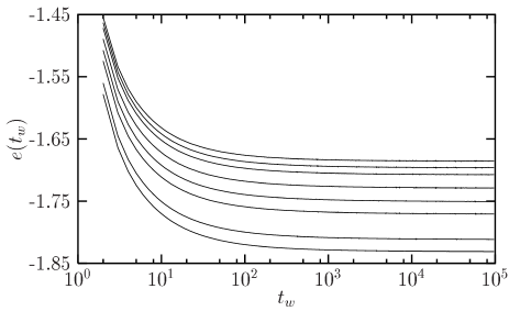
Figure 1: The time dependence of the energy density for temperatures $T=0.16$, 0.15, 0.14, 0.12, 0.10, 0.08, 0.04 and 0.02 (from top to bottom) reveals the aging of the system in its low temperature phase, $T\leq T_{c}\simeq 0.16$.

It is a central feature of glassy materials that they do not reach thermal equilibrium on experimental time scales when they are quenched to their “glassy” phase. The main consequence is that physical quantities keep evolving with time as the system tries to reach equilibrium, which is known as “aging”, a term invented by the polymer glass community struik .

An obvious manifestation of this out-of-equilibrium dynamics is therefore the time dependence of physical observables. In our case, it is easy to follow the evolution of the energy density,

$$e(t_{w})=\left\langle\frac{1}{N}H\right\rangle.$$ (4)

That the system ages at all temperatures studied here is indeed clear from Fig. 1 where at each temperature $T\in[0.02,0.16]$ the time dependence of $e(t_{w})$ is evident.

III.2 Two-time autocorrelation functions

The evolution with time of physical observables implies that the dynamics of the system is not time translationally invariant. Early studies on polymeric glasses showed that two-time quantities reveal the aging behavior of the system much more strikingly struik , so that two-time correlation or response functions are widely studied in aging glassy materials.

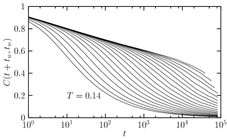
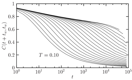
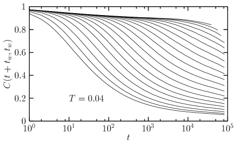
Figure 2: Autocorrelation function of the spins, Eq. (5), for $L=60$, as a function of the time difference $t$ for various waiting times $t_{w}$ logarithmically spaced in the interval $t_{w}\in[2,57797]$ (from left to right). The temperature is $T=0.14$, 0.10 and 0.04 (from top to bottom).

The simplest two-time quantity that has been studied numerically in spin glasses is the autocorrelation function of the spins defined by

$$C(t+t_{w},t_{w})={1\over N}\sum_{i}\langle{\bf S}_{i}(t+t_{w})\cdot{\bf S}_{i}(t_{w})\rangle.$$ (5)

This function is represented as a function of the time difference $t$ for various waiting times $t_{w}$ and various temperatures in Fig. 2.

The first and main observation from Fig. 2 is that this two-time quantity is not a function of the time difference only, as it would be in an equilibrium system, $C(t+t_{w},t_{w})\neq C(t)$. This is just another way of saying that the system is aging, but much more information can be extracted from this correlator.

In more detail, the shape of the curves shown in Fig. 2 is similar to what is commonly observed in many materials. For small time differences, $t\ll t_{w}$, the curves for various $t_{w}$ superpose, implying that the dynamics is time translationally invariant in this time regime, reminiscent of some sort of “local” or “quasi” equilibrium. This will be clarified below. Moreover, we find that for all $T\leq 0.10$, the curves in this time regime are consistent with the existence of a “plateau”. At $T=0.10$, the plateau starts to be visible at time differences $t\sim 10^{3}-10^{4}$ only, but its existence becomes clearer at lower temperatures. In mathematical terms, this means that the Edwards-Anderson parameter defined as

$$q_{\rm EA}=\lim_{t\to\infty}\lim_{t_{w}\to\infty}\lim_{L\to\infty}C(t+t_{w},t_{w}),$$ (6)

is finite and positive, $q_{\rm EA}>0$. It is important that the system is large enough that it can be considered effectively infinite for the values of $t$ and $t_{w}$ used. If the system is not large enough, the overall direction of the spins will wander randomly during the simulation, since there is no energy cost to a global rotation, with the result that $\lim_{t\to\infty}\lim_{t_{w}\to\infty}C(t+t_{w},t_{w})=0$ at fixed $L$. It is clear from Fig. 2 that $q_{\rm EA}$ is a decreasing function of temperature, with $q_{\rm EA}(T\to 0)=1$. At higher temperatures, we do not observe a plateau, presumably because our time window is too small, as can be guessed from comparing the curves at $T=0.14$ and $T=0.10$ in Fig. 2.

Although a plateau is expected, because equilibrium measurements indicate spin glass order below $T_{c}$, we recall that no such plateau can be unambiguously observed in the Ising spin glass in three dimensions, where the short time regime is well-described by a pure power law rieger ; BB . A non-zero $q_{\rm EA}$ indicates the existence of spin glass phase where spins are frozen in random directions, and the observation of a plateau in the spin autocorrelation function in Fig. 2 is the first evidence of a standard spin glass phase in the model in Eq. (2) using non-equilibrium techniques. For the Ising spin glass, analogous evidence for a transition is currently missing. Experimentally, plateaus are also hardly visible in two-time correlation or response functions, but this is probably due to the narrow experimental time window. The existence of a plateau can be, however, experimentally revealed through a scaling analysis of two-time quantities review1 ; review1_1 .

Turning to the large time regime, $t\gg t_{w}$, we observe that curves at various waiting times do not superpose at all in this regime at any temperature, fully revealing the aging nature of the dynamics. As in many glassy materials, it is clear that the time decay of $C(t+t_{w},t_{w})$ becomes slower when the waiting time increases. The physical interpretation is simple: since the relaxation time of the sample is infinite, the only relevant time scale is the age of the sample $t_{w}$ which imposes an age-dependent relaxation time: the older the sample, the slower its relaxation becomes. We shall discuss in the next section the scaling behavior of these curves.

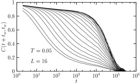
Figure 3: Autocorrelation function of the spins for $T=0.05$ and $L=16$ show that the use of too small a system size yields stationary data for $t_{w}>10^{4}$, not observed in the larger system used in Fig. 2.

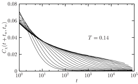
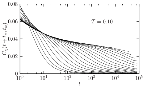
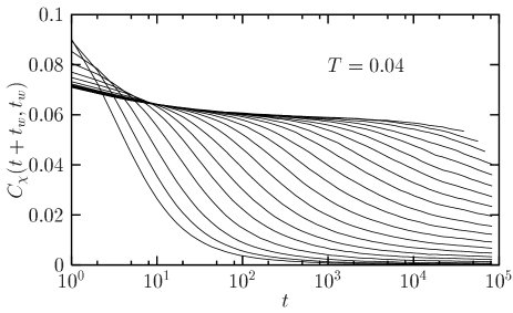
Figure 4: Autocorrelation function of the chirality, Eq. (7), as a function of the time difference $t$ for various waiting times $t_{w}$ logarithmically spaced in the interval $t_{w}\in[2,57797]$ (from left to right). The temperature is $T=0.14$, 0.10 and 0.04 (from top to bottom).

The long time behavior found here is qualitatively very different from the one reported by Kawamura kawa who argues that the spin autocorrelation function becomes stationary at large times, even at temperatures as low as $T=0.05$. This fact was later corrected by Matsubara et al. matsu who noted that a global rotation or “drift” of the system could affect the dynamics, and produced curves similar to ours by “subtracting” by hand a global rotation of the spins. This is more simply interpreted as the system being too small for the order of limits in Eq. (6) to apply. Our results for an $L=16$ system, plotted in Fig. 3, are consistent with those of Kawamura kawa , and show stationary behavior at long times. By contrast, for $L=60$, the spin autocorrelation function shown in Fig. 2, does not reach stationarity in the same time window even for temperatures as high as $T=0.16$ and without subtracting a global rotation of the spins. This shows that one of Kawamura’s numerical arguments in favor of a spin-chirality decoupling kawa stems from data on too small a size. Similar finite-size effects are most probably also at work in Refs. kawa2, ; kawa3, .

We now present data for the autocorrelation function of the chirality,

$$C_{\chi}(t+t_{w},t_{w})=\frac{1}{N}\sum_{i}\langle\chi_{i}^{\mu}(t+t_{w})\chi_{i}^{\mu}(t_{w})\rangle.$$ (7)

Since the system is isotropic, $C_{\chi}$ does not depend on $\mu$ and we have also averaged the data over the three directions of space. Our results are shown in Fig. 4 for the same parameters as for the spins. The main conclusion from Fig. 4 is that chiralities have essentially the same behavior as the spins. We observe a stationary decay at small $t$, followed by a slower, waiting time dependent decay at large times. As for the spins, the appearance of a plateau is clear within our time window for $T\leq 0.10$, indicating the existence of a non-zero Edwards-Anderson parameter for chirality,

$$q_{\chi{\rm EA}}=\lim_{t\to\infty}\lim_{t_{w}\to\infty}\lim_{L\to\infty}C_{\chi}(t+t_{w},t_{w}),$$ (8)

which also grows when $T$ decreases. This is expected since we have found above that spins freeze, which implies that chiralities freeze as well.

III.3 Time is length

Figure 5: The relative orientation of the spins in two copies of the system, Eq. (9), is encoded on a grey scale in a $60\times 60\times 60$ simulation box at three different waiting times $t_{w}=2$, 27 and 57797 (from top to bottom) at temperature $T=0.04$. The growth of a local random ordering of the spins is evident.

Figure 6: The sign of the chiral local overlaps in two copies of the system, Eq. (10), is encoded on a black and white scale in a $60\times 60\times 60$ simulation box at three different waiting times $t_{w}=2$, 27 and 57797 (from top to bottom). The temperature is $T=0.04$, and we have chosen $\mu=x$. The actual configurations are the same as in Fig. 5, but the chiral ordering, corresponding to the spin ordering observed there, is hardly visible.

The key problem is to understand the subtle slow changes that the system undergoes: what does “old” or “young” really mean for the sample? To answer this question, we turn to a spatial description of the aging dynamics.

The decomposition of the decay of autocorrelation functions into a fast stationary process and a slow non-stationary one directly suggests the existence of some sort of local equilibrium within the sample: a spin appears locally equilibrated (short-time dynamics) although the sample as a whole is still far from equilibrium and evolves towards equilibrium (long-time dynamics).

It is possible to illustrate this last statement, as was done in the Ising case rieger . Because of the disorder, the spin orientations in an equilibrium configuration are random, so that it is impossible to detect any domain growth by simply looking at the spin directions. However, two copies of the system, $a$ and $b$, evolving independently but with the same realization of the disorder, will reach correlated equilibrium configurations, so that the orientation of the spins in one copy can be compared with those in the second copy.

It is therefore useful to define the local relative orientation of the spins as

$$\cos\theta_{i}(t_{w})={\bf S}_{i}^{a}(t_{w})\cdot{\bf S}_{i}^{b}(t_{w}).$$ (9)

In Fig. 5 we present snapshots where this quantity is encoded on a grey scale. Comparing three successive times, it becomes clear that aging is nothing but the growth with time of a local random ordering of the spins imposed by the disorder of the Hamiltonian fh ; huse . Notice that the “domains” observed in Fig. 5 have highly irregular boundaries, which will influence the behavior of the spatial correlators discussed below.

Next we focus on chiral degrees of freedom, and similarly define a chiral local overlap as

$$q_{\chi i}^{\mu}(t_{w})=\chi_{i}^{\mu,a}(t_{w})\chi_{i}^{\mu,b}(t_{w}).$$ (10)

In Fig. 6, we present snapshots where this quantity is encoded on a black and white scale, i.e. we represent the quantity ${\rm sgn}(q_{\chi i}^{\mu})$ for $\mu=x$. Different space directions would give similar plots. Although a chiral ordering must follow the spin ordering observed in Fig. 5, this is hardly visible by the eye and the system appears much more disordered in this chiral representation. We interpret this as stemming from the fact that spins are actually not “very” correlated within the dynamic correlation length (see the next subsection), and so the chiralities, which involve three spins, are even less correlated.

III.4 Four-point correlation functions

We now go beyond qualitative pictures of black and white domains and measure the dynamic correlation length associated with the mean domain size observed in Figs. 5 and 6.

First, we generalize the two-site, two-replica correlation function (which is therefore a “four-point” object) studied in the Ising case rieger to the case of Heisenberg spins as

$$C_{4}(r,t_{w})={1\over N}\sum_{i}\langle{\bf S}_{i}^{a}(t_{w})\cdot{\bf S}_{i+r}^{a}(t_{w})\,\,{\bf S}_{i}^{b}(t_{w})\cdot{\bf S}_{i+r}^{b}(t_{w})\rangle.$$ (11)

This function measures correlations of the relative orientation of two spins separated by a distance $r$ at time $t_{w}$, just as the structure factor does in a pure ferromagnet. Note that $C_{4}(r,t_{w})$ is invariant under global rotation of the spins in either copy, and so is independent of the wandering of the overall spin orientation which can affect the two-time autocorrelation functions discussed in Sec. III.2. However, there will be a change of behavior in $C_{4}(r,t_{w})$ when $t_{w}$ is sufficiently large that the dynamic correlation length becomes comparable to the system size $L$, since the system then equilibrates.

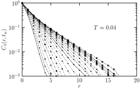
Figure 7: The two-site two-replica correlator for the spins defined in Eq. (11) as a function of $r$ for various waiting times logarithmically spaced in the interval $t_{w}\in[2,57797]$ (from left to right). The temperature is $T=0.14$, 0.10 and 0.04 (from top to bottom). Note that the range of the $r$ axis changes with temperature as a result of a slower growth of the dynamic correlation length at lower temperature. A non-exponential decay is also evident from these curves.

We present the space dependence of $C_{4}(r,t_{w})$ for various $t_{w}$ and three different temperatures in Fig. 7. These data obviously confirm the visual impression of the snapshots in Fig. 5. At a given temperature, the decay of $C_{4}(r,t_{w})$ with $r$ becomes slower at larger $t_{w}$, indicating the growth with time of a dynamic correlation length, $\ell(T,t_{w})$, sometimes also referred to as a “coherence length”. Physically, this means that an “older” system exhibits slower dynamics because of a larger dynamic correlation, very much as in standard coarsening phenomena fh .

A second piece information we get from Fig. 7 is that the growth of $\ell(T,t_{w})$ is strongly dependent on temperature, since much larger length scales can be equilibrated at $T=0.14$ than at $T=0.04$. This is expected in a disordered system where thermal activation is likely to play a role, and we shall quantify this statement in the next section. We also note that much smaller length scales are reached in the same time window in the Ising spin glass, both in three and four dimensions, where plots similar to Fig. 7 typically stop rieger ; BB at $r=5$–$10$, instead of $r=20$–$30$ used here.

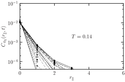
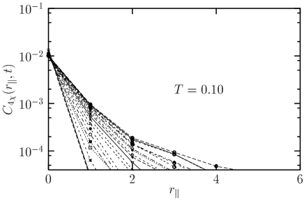
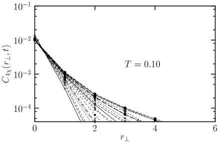
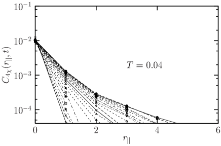
Figure 8: The two-site two-replica correlator for the chiralities (12) as a function of $r$ for various waiting times logarithmically spaced in the interval $t_{w}\in[2,57797]$. The temperature is $T=0.14$, 0.10 and 0.04 (from top to bottom). For $T=0.10$ we show both $C_{4\chi}(r_{\parallel},t_{w})$ and $C_{4\chi}(r_{\perp},t_{w})$ which exhibit similar behavior. Note that the range of the $r$ axis is much smaller than that for the spin correlator in Fig. 7.

A third piece of information is that the spatial decay of $C_{4}(r,t_{w})$ is clearly not exponential, since the latter would correspond to straight lines in the lin-log representation adopted in Fig. 7. Moreover, a closer inspection of the data shows that, as for the time decay of the autocorrelation functions, they can be decomposed in a short-distance decay, $r<\ell(T,t_{w})$ where the curves at various $t_{w}$ merge, and a long-distance one, $r>\ell(T,t_{w})$, which becomes slower at larger $t_{w}$. This confirms the intuition that spins are indeed in local equilibrium on short length scales, but that the system as a whole is not equilibrated. We note that even the local equilibrium part of the decay seems to be non-exponential, which might be connected to the strongly irregular nature of the domains observed in Fig. 5.

Finally note that the correlator in Eq. (11) is symmetric about $L/2=30$ due to periodic boundary conditions. A look at Fig. 7 justifies our use of a system size $L=60$ since even for the largest waiting time and the largest temperature studied here, we are in the regime where $\ell(T,t_{w})<L/2$, so that our results are not affected by finite size effects.

We now turn to the chiral degrees of freedom and define corresponding two-site, two-replica spatial correlations of the chirality as

$$C_{4\chi}(r,t_{w})={1\over N}\sum_{i}\langle\chi_{i}^{\mu,a}(t_{w})\chi_{i+r}^{\mu,a}(t_{w})\chi_{i}^{\mu,b}(t_{w})\chi_{i+r}^{\mu,b}(t_{w})\rangle.$$ (12)

In the following we distinguish between two correlators $C_{4\chi}(r_{\parallel},t_{w})$ and $C_{4\chi}(r_{\perp},t_{w})$ if $r$ is taken in a direction parallel or perpendicular to $\mu$, respectively.

Our results for the correlators (12) are presented in Fig. 8. As for the spins, the spatial decay becomes less fast at larger $t_{w}$, indicating a gradual random ordering of the chiralities. Although this ordering was not visible on the snapshots presented in Fig. 6, appropriate correlators not surprisingly perform better than the eye. Chiral ordering is anyway expected since ordering of the spins implies the one of chiralities. In agreement with the visual observations, however, we find that spatial correlations of chiralities are much weaker than for the spins and correlators are numerically indistinguishable from noise beyond $r\sim 4$. As a result, we did not attempt to perform a detailed scaling analysis of spatial correlations of the chirality. Again, we interpret this as being due to the fact that chiralities are less correlated because they involve three spins on a length scale $r=2$.

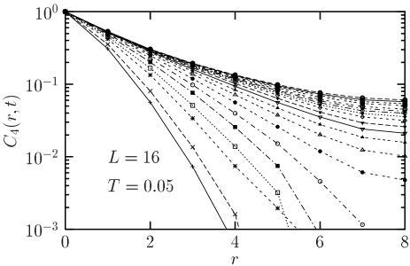
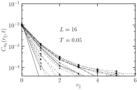
Figure 9: Two-site, two-replica functions for spins (top) and chiralities (bottom) at $T=0.05$ and $L=16$. While the bottom figure is very similar to Fig. 8, the top figure is very different (note in particular the different $r$-range used in both cases).

Results for the spin and chiral two-site, two-replica correlators for $L=16$, the size studied by Kawamura kawa , are shown in Fig. 9. By comparing the top of Fig. 9 with Fig. 7 which is for $L=60$, we see that the behavior of the spin function is very strongly size dependent. Physically this is because the smaller system size comes to, or approaches, equilibrium on the time scale of the simulation, whereas the larger size does not. However, the data for the chiral function for $L=16$ in the bottom part of Fig. 9 is not very different from that for $L=60$ shown in Fig. 8. This observation explains why Kawamura kawa found that chiral autocorrelation does not stop aging while spin autocorrelation does.

Although we have not been able to precisely estimate the dynamic correlation length associated with chiral order, the fact that we cannot measure correlations beyond $r\sim 4$, while we can estimate spin correlations up to $r\sim 25$ shows that spin correlations are much stronger in the whole temperature range that we have investigated, $T\leq 0.16$. This implies that we find no temperature regime below $T=0.16$ where chiral order manifests itself unaccompanied by simultaneous spin ordering as a spin-chirality decoupling scenario naturally predicts. Hence, although the present non-equilibrium approach says nothing about equilibrium behavior in the thermodynamic limit, an important conclusion of this whole section is that, when a proper system size is used, dynamical studies of the Heisenberg spin glass are more simply interpreted in terms of a simultaneous phase transition at $T_{c}\simeq 0.16$ for both spin and chiral degrees of freedom.

IV Scaling of dynamic functions

The study of several space-time correlators of the previous section leads to the conclusion that for $T\leq 0.16$, spins of the Heisenberg spin glass gradually freeze with time in random orientations dictated by the quenched disorder, naturally followed by chiral degrees of freedom. This behavior is qualitatively similar to that of the Ising spin glass. In this section, we study the scaling behavior of dynamic functions defined for the spin degrees of freedom, to get a quantitative description of its aging dynamics, and compare the results with numerical studies of the Ising spin glass and with experiments.

IV.1 Spatial correlations

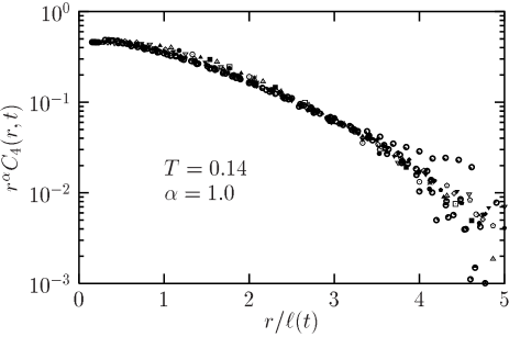
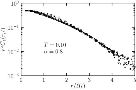
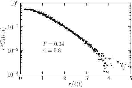
Figure 10: Rescaled four-point functions of the spins according to the scaling form (13), and using (14), for temperatures $T=0.14$, 0.10 and 0.04 (from top to bottom). Parameters and symbols are the same as in Fig. 7.

We start our scaling analysis with the study of spatial correlations of the spins. This choice is dictated by theoretical considerations, since scaling theories of aging dynamics show that time correlations have natural scaling forms when expressed as a function of the dynamical correlation length $\ell$ fh ; encorejp ; yosh ; surf ; yosh5_1 ; yosh5 , so that its knowledge is of primary importance in this study.

Following the physical discussion of the previous section, it is natural to suggest the following decomposition of $C_{4}(r,t_{w})$ between a “locally equilibrated” and an “aging” part,

$$C_{4}(r,t_{w})\simeq C_{4{\rm eq}}(r)\,C_{4{\rm aging}}\left(\frac{r}{\ell(T,t_{w})}\right),$$ (13)

with $C_{4{\rm aging}}(x\to 0)\sim\mbox{constant}$, and $C_{4{\rm aging}}(x\to\infty)=0$. As in studies of the Ising spin glass BB ; enzo , we found that the functional forms

$$C_{4{\rm eq}}(r)\simeq r^{-\alpha(T)},$$ (14)

and

$$C_{4{\rm aging}}(x)\simeq\exp\left(-x^{\beta}\right),\quad\beta>1,$$ (15)

represent the data quite well, so that a plot at fixed $T$ of $r^{\alpha}C_{4}(r,t_{w})$ versus the scaling variable $r/\ell$ should collapse the data for all times $t_{w}$. Such scaling plots are indeed presented in Fig. 10. Although the data collapse is quite good, small deviations can be observed in these scaling plots. This might be due to the fact that corrections to scaling arise at small waiting times where the coherence length is still small, so that a scaling regime defined by $\ell\gg 1$ is not entered yet. Similar scaling plots were obtained for the Ising spin glass BB ; enzo , although on a more restricted spatial range.

Table 1: Temperature variation of the exponent $\alpha$ of the power law in Eq. (14) of the spatial correlations, and the exponent $\mu$ which occurs in the scaling of the autocorrelation function, see Eq. (26).

$T$	0.16	0.15	0.14	0.12	0.10	0.08	0.04	0.02
$\alpha$	1.1	1.05	1.0	0.9	0.8	0.8	0.8	0.8
$\mu$	0.97	0.98	0.98	1.0	1.01	1.03	1.07	1.09

The temperature variation of the exponent $\alpha(T)$ in Eq. (14) is shown in Table 1. At very low temperatures, $T\leq 0.10$, it seems to be roughly constant at about $0.8$. The same trend is also found in the Ising spin glass, although there the exponent sticks to the value $0.5$. At $T_{c}$ the scaling forms in Eqs. (13), and (14) are also expected to hold with $\alpha$ related to the anomalous exponent $\eta$ via the relation

$$\alpha(T_{c})=d-2+\eta.$$ (16)

Our estimate for $\eta$ is therefore

$$\eta\approx 0.1.$$ (17)

We cannot estimate error-bars on this value since it results from a somewhat arbitrary scaling procedure.

As for the Ising case, we find evidence that

$$\lim_{r\to\infty}\lim_{t_{w}\to\infty}\lim_{L\to\infty}C_{4}(r,t_{w})=0,$$ (18)

since $\alpha>0$. Here $L$ has to be much larger than $\ell(T,t_{w})$, otherwise the system comes to equilibrium, and we get a non-zero value simply because the system has spin glass order (see again Fig. 9).

From the point of view of the droplet picturefh (which has a single ground state plus those related by global symmetry), Eq. (18) is puzzling since one expects $\lim_{r,t_{w},L\to\infty}C_{4}(r,t_{w})=\langle q^{2}\rangle_{\rm eq}=q_{\rm EA}^{2}$. The data in Figs. 7 and 8 are clearly inconsistent with the large $r$ limits being equal to $\langle q^{2}\rangle_{\rm eq}$ as estimated from the autocorrelations in Figs. 2 and 4. However, Eq. (18) has been justified BB ; enzo within the replica symmetry breaking (many-state, “RSB”) picture BB ; enzo . The argument reviewsimu is that an equilibrium calculation of the correlator (11) within a replica symmetry breaking approach predicts power law behavior like Eq. (14) with a non-zero $\alpha$ in the “zero-overlap” sector cyrano . However, this argument is really for equilibrium fluctuations, and it is not obvious how to translate this result to the non-equilibrium situation of interest here. In particular, a restricted average over the “zero-overlap” sector cannot be justified by the sole (trivial) observation that the global overlap is zero in the aging regime reviewsimu .

To distinguish between the single and many states pictures, one should perform local measurements and show that local properties are (in)consistent with the existence of a single equilibrium state fisher . The correlator in Eq. (11) can do this, using the (square of the) relative spin orientation as a local physical observable. Although, as discussed above, it is not clear to us that the argument often given for a power law variation within RSB theory is correct, the droplet theory makes the clear prediction fh that Eq. (11) tends to a constant, $q_{\rm EA}^{2}$, for $t_{w}\to\infty$. Hence the results of our simulations, which fit the power law variation in Eq. (14) with $\alpha>0$, may be closer to the RSB “many states” picture, at least on the time and length scales being probed. Theoretical studies of the two-site, two-replica correlation function, $C_{4}$, using the Migdal-Kadanoff approximation in the spirit of Refs. yosh5_1 ; martin , would be very valuable.

IV.2 Length scales

From the scaling behavior of $C_{4}(r,t_{w})$, we obtain a practical definition of the dynamical correlation length of the spins as the quantity leading to the best collapse of the data in Fig. 10. An obvious problem is that the results for $\ell$ are affected by the uncertainty in the value of $\alpha$, as is also the case in the Ising spin glass. In particular, this makes it impossible to estimate error-bars on our results for $\ell$. The evolution with time of the coherence length at various temperatures is presented in Fig. 11, where a log-log representation is used. We find that $\ell$ grows with time, in a temperature dependent manner, as was anticipated above.

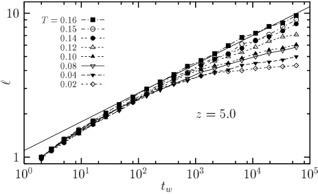
Figure 11: Growth law of the coherence length at different temperatures. The data are represented by points and lines. The straight line is a power law fit to the data at large times for $T=0.16$, $\ell\sim t_{w}^{1/z}$, with $z\approx 5.0$.

From non-equilibrium critical dynamics arguments, one expects $\ell\sim t_{w}^{1/z}$, where $z$ is the critical dynamic exponent. An activated scaling, $\ell\sim(T\ln t_{w})^{1/\psi}$, is more naturally expected at low temperatures, where $\psi$ is the so-called barrier exponent fh . Moreover, at a given temperature $T\lesssim T_{c}$, we expect a crossover from a critical (power-law) regime at short times to an activated regime at large times, which occurs at shorter times for lower temperatures.

All these theoretical expectations can successfully be observed in our numerical results in Fig. 11. For $T=0.16$, a power law behavior is consistent with the data at large enough times, with

$$z\approx 5.0.$$ (19)

Here again, we did not attempt to define error-bars on the value of the exponent. The value $z\approx 7.0$ was found using the same method in the Ising spin glass BB . It is the smaller value of the dynamic exponent which allows larger length scales to be reached in the Heisenberg model than in the Ising model, as was noted above.

Clearly, at low $T$, the long-time behavior is not consistent with a power law and the bending of the curves is indeed compatible with a logarithmic growth law. Note that even at the lowest temperature we have simulated, $T=0.02$, the first two decades of waiting times give a growth law very similar to the one obtained at $T=0.16$, indicating that the “true” activated behavior is entered in the last three decades of the simulations only. This is consistent with the corrections to scaling observed in the spatial correlators, recall Fig. 10. For this reason, our data do not allow a precise determination of the barrier exponent $\psi$ from a logarithmic fit to the growth law which contains too many free parameters. Likewise, the interpolation law between critical and activated regimes encorejp ; BB ; dupuis ; yosh6 ,

$$t_{w}\sim t_{o}\left(\frac{\ell}{\ell_{o}}\right)^{z}\exp\left[\frac{\Upsilon_{o}}{T}\left(\frac{\ell}{\xi(T)}\right)^{\psi}\right],$$ (20)

which was used in earlier studies, does not account for the crossover seen in our data. In this expression, $\xi\sim|T-T_{c}|^{-\nu}$ where $\nu$ is the critical exponent for the equilibrium correlation length, and $\ell_{o}$, $t_{o}$ and $\Upsilon_{o}$ are microscopic length, time and energy scales respectively.

The conclusion is that larger time scales need to be studied to establish a more quantitative description of the growth law for $\ell$, but this is difficult because it would require a huge amount of computer time, as one would have to work with even larger system sizes.

It is nevertheless possible to compare these results with the Ising spin glass. In Fig. 12, we replot the data of Fig. 11 together with published data obtained in the Ising Edwards-Anderson model BB . We use the representation adopted in Ref. bert, to compare similar experimental data in Heisenberg and Ising samples, and plot $\ell$ versus $\frac{T}{T_{c}}\ln(t_{w})$ in a lin-log scale. In this representation, data at different times and temperatures collapse if $\ell\sim t_{w}^{zT/T_{c}}$, a growth law advocated in some early studies yosh2 ; enzo ; orbach . We recognize from Fig. 12 that this functional form indeed reasonably accounts for the Ising data but not at all for the Heisenberg ones. Also, Fig. 12 clearly confirms that larger length scales can be studied in the Heisenberg model than in the Ising model in three dimensions. Further, we find in the Heisenberg model clear evidence of an activated, logarithmic growth law, shown by the downward curvature in the data in Figs. 11 and 12 at low temperature. This effect is not observed in the Ising model, see Fig. 12.

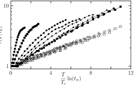
Figure 12: Comparison of the growth of the dynamic correlation length in Heisenberg (data from Fig. 11) and Ising (published data from Ref. BB, ) models. We use the experimental representation of Ref. bert, , plotting $\ell$ versus $(T/T_{c})\ln(t_{w})$. Heisenberg data are represented with closed symbols for $T=0.16$, 0.15, 0.14, 0.12, 0.10, 0.08, 0.04, 0.02 (from right to left), $T_{c}\simeq 0.16$. Ising data are represented with open symbols for $T=0.95$, 0.855, 0.76, 0.665, 0.57, 0.475 (from right to left), $T_{c}\simeq 0.95$.

Turning to experiments, direct measurements of the dynamical correlation length are obviously impossible since the correlator in Eq. (11) can not be measured experimentally. The least indirect method we are aware of was first suggested in Ref. orbach, and used more recently in a variety of samples bert . It consists of a dynamic estimate of the number of spins that relax in a coherent manner probed through a magnetic perturbation. Results bert on both Heisenberg-like and Ising-like systems were gathered in the same representation as Fig. 12 (see Fig. 4 in Ref. bert, ). Our results are useful to understand the trends found in experiments. In particular, in Ising samples, the dynamical correlation length is experimentally found to be smaller but to grow faster with increasing time than in Heisenberg samples bert . We will now see that this can be understood from the data in Fig. 12.

The Ising spin glass has a larger dynamical exponent $z$, which means that its dynamical correlation length initially grows more slowly, since the straight-line data at $T=T_{c}$ in Figs. 11 and 12 have slope $1/z$. At intermediate temperatures where experiments are usually carried out, the system leaves the critical regime after a crossover time scale $t_{\rm c}$ given by

$$t_{\rm c}\sim|T-T_{c}|^{-z\nu}.$$ (21)

For the Gaussian Ising and Heisenberg Edwards-Anderson models in three dimensions, it is found that BB ; peternew

$$z\nu|_{\rm Ising}\simeq 10.5,\quad z\nu|_{\rm Heisenberg}\simeq 5.5,$$ (22)

in fair agreement with the experimental values reported in Ref. bert, : $10.5$ for the Ising system Fe_0.5Mn_0.5TiO₃, and $7$ and $5$ respectively for the Heisenberg systems CdCr_1.7In_0.3S₄ and Ag:Mn $2.7\%$. Eqs. (21) and (22) show that Heisenberg systems leave the critical region at much earlier times than Ising samples. For $t>t_{c}$ there is a crossover, visible in Fig. 11 and the Heisenberg data in Fig. 12, to presumably activated behavior, $\ell\propto(\ln t)^{1/\psi}$, where $\psi$ is the barrier exponent. It can be argued BB that this crossover rationalizes the apparent $T$-dependent dynamic exponent $zT/T_{c}$ observed in the Ising model. Hence, in the experimental time window, Heisenberg samples lie deeper in the activated regime where large length scales have been reached but further growth is extremely slow. In the range of times available in the simulations, we do not see the phenomenon observed experimentally bert that $\ell$ increases more slowly for Heisenberg systems than for Ising systems. However, at longer times, such as those in the experiments, we expect this would occur since the Heisenberg model is clearly entering the activated region where $\ell$ increases only logarithmically with $t$. Hence our data provides a consistent explanation of the results of Ref. bert, .

IV.3 Autocorrelation functions

Finally, we study the scaling behavior of the spin autocorrelation function. This function has been much studied in Ising spin glasses, and has recently been measured in experiments herisson which have usually focused on the more easily accessible thermo-remanent magnetization review1 ; review1_1 . Both functions are believed to exhibit similar scaling behavior.

As we did for the spatial correlations, it is natural to decompose $C(t+t_{w},t_{w})$ into an equilibrium and an aging part,

$$C(t+t_{w},t_{w})\simeq C_{\rm eq}(t)\,\,C_{\rm aging}\left(\frac{h(t+t_{w})}{h(t_{w})}\right),$$ (23)

where $h(t)$ is an unknown function increasing with time, and the scaling function $C_{\rm aging}$ has the following limits: $C_{\rm aging}(x\to 0)=\mbox{constant}$ and $C_{\rm aging}(x\to\infty)=0$. Two simple expectations for the aging part are the following. (i) $h(t)=t$ leading to a simple $t/t_{w}$ scaling of the aging part of the data; (ii) $h(t)=\ell(t)$, the dynamical correlation length, which is the basic outcome of scaling theories fh , and is also obtained in coarsening phenomena. It is important to notice that although popular, $t/t_{w}$ is not theoretically expected to hold in spin glasses, as already emphasized BB . The natural choice of $h(t)=\ell(t)$ does not lead to $t/t_{w}$ scaling if the dynamics involves barrier activation because then $\ell(t)$ grows logarithmically with time, though $t/t_{w}$ scaling is obtained for critical dynamics where $\ell(t)\propto t^{1/z}$. Furthermore, exactly solvable models have demonstrated the possibility of more general scaling forms reviewth ; cuku1 ; cuku2 that we also discuss below.

In analysis of experimental data, deviations from $t/t_{w}$ scaling are often described phenomenologically by the replacement

$${t\over t_{w}}\ \to\ t_{w}^{1-\mu}\,f\left({t\over t_{w}}\right)\,,$$ (24)

as the scaling variable in $C_{\rm aging}$, where $\mu$ is an exponent (in practice close to unity) and $f$ a scaling function. The simplest choice would be $f(x)=x$, but it is more common to take

$$f(x)={1\over 1-\mu}\left[\left(1+x\right)^{1-\mu}-1\right]\,,$$ (25)

so Eq. (24) becomes

$${t\over t_{w}}\ \to\ u(t_{w},t)={1\over 1-\mu}\left[\left(t+t_{w}\right)^{1-\mu}-t_{w}^{1-\mu}\right]\,,$$ (26)

since this attempts to take into account the fact that the real age of the sample during the measurement is $t+t_{w}$ rather than $t_{w}$, see e.g. Ref. cool, . This function $u(t_{w},t)$ corresponds to

$$h(t)=\exp\left[\frac{t^{1-\mu}}{1-\mu}\right]$$ (27)

in Eq. (23), and reduces to $t_{w}^{1-\mu}(t/t_{w})$ for $t\ll t_{w}$.

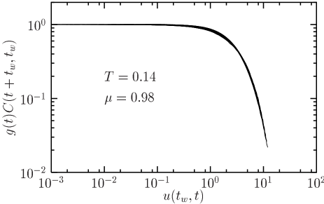
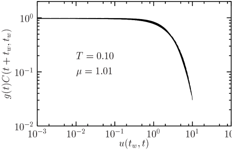
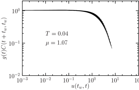
Figure 13: Spin autocorrelation functions rescaled using Eqs. (23), (26) and (28). The temperature $T$ and the exponent $\mu$ are indicated in each figure.

Contrary to the Ising spin glass, we find that the initial decay of the correlation function is better described by a logarithmic behavior than by a power law, and we take

$$C_{\rm eq}(t)=a-b\,\log(t)\equiv g(t),$$ (28)

where $a$ and $b$ are two temperature dependent parameters describes the data very well. This can be recognized from the initial linear aspect of the data in Fig. 2 where a log-lin representation was used. Experimentally also, an initial power law decay of the data is generally adopted, but the numerical value of this exponent is extremely small, typically $<0.10$, so that differences from a logarithmic behavior are probably small.

Although the low temperature data in Fig. (2) show evidence for a plateau, i.e. a non-zero value at large $t_{w}$ and $t$, Eqs. (23) and (28) do not lead to a true plateau. However, Eq. (23) is sufficient to fit the data and has one less parameter than a function with a plateau. Also, as discussed many times in the Ising case BB ; ricci , the use of an additive scaling in Eq. (23) is in principle more appropriate, but it too contains one more free parameter. In practice, data taken over a limited time window are usually not sufficient to independently fix all free parameters when such an additive scaling is used ricci . We find indeed that our data can be equally well fitted with an additive and a multiplicative form and both lead to similar results as far as the scaling properties of the aging part are concerned. Here, we shall present results with a multiplicative scaling only.

With $(a,b,\mu)$ as free parameters, we have been able to get a satisfactory collapse of the numerical data at all waiting times and temperatures by plotting $g(t)\,C(t+t_{w},t_{w})$ as a function of the scaling variable $u(t_{w},t)$. Representative results are shown in Fig. 13.

We find that the scaling function $C_{\rm aging}(x)$ behaves at large $x$ as

$$C_{\rm aging}(x)\sim x^{-\lambda_{1}},\quad T\lesssim T_{c},$$ (29)

$$C_{\rm aging}(x)\sim(\log x)^{-\lambda_{2}},\quad T\ll T_{c},$$ (30)

with two temperature dependent exponents $\lambda_{1},\lambda_{2}>0$. We find for instance that $\lambda_{1}(T=0.14)\approx 0.5$, $\lambda_{1}(T=0.12)=0.4$, $\lambda_{2}(T=0.04)\approx 2$, and $\lambda_{2}(T=0.02)\approx 1.5$. The existence of two different scaling forms is another evidence that the dynamics crosses over from a critical to an activated regime when $T$ is decreased from $T_{c}$ down to $0$. Again, this is not the case in the Ising spin glass which is well described by a power law of the autocorrelation at large times in the whole low temperature phase, $T\leq T_{c}$ rieger .

An outcome of the scaling procedure of Fig. 13 is therefore an estimate of the temperature dependence of the exponent $\mu$, and we report this in Table 1. We observe a systematic increase of $\mu$ when the temperature decreases. For $T=T_{c}$, we find $\mu<1$, a behavior which has been called “subaging”. When decreasing the temperature, however, $\mu$ becomes equal to 1 around $T\approx 0.12$, and “superaging”, corresponding to $\mu>1$, is found at still lower temperatures.

In the Ising spin glass, the situation is again different since data in three dimensions indicate that the scaling variable $t/t_{w}$ can be used, corresponding to $\mu=1$, in the whole low temperature phase BB ; jimenez . In four dimensions, however, the same tendency as here is found with $\mu=1$ close to $T_{c}$ but $\mu>1$ at lower temperatures BB . More puzzling is the experimental situation, since there one has $\mu<1$ and the temperature dependence is the opposite with $\mu$ decreasing when the temperature is lowered review1 . As discussed in Refs. BB, ; cool, , however, experimental quenches involve a finite cooling rate, so that laboratory aging experiments are in fact temperature-shift protocols. We will therefore come back to subaging behavior found in experiments in our future paper prep .

This multiplicity of experimental and numerical behaviors obviously requires some discussion. As described above, there is no obvious theoretical reason to expect a perfect $t/t_{w}$ scaling in spin glasses aging at low temperatures, so that deviations from this simple behavior should not come as a surprise. Moreover, the rescaling obtained in Fig. 13 is purely phenomenological, and must be interpreted as an effective description of the data rather than a fundamental one. This is consistent with Kurchan’s work showing that persistent superaging encoded by Eqs. (23) and (27) with $\mu>1$ is strictly impossible jorge .

For $T=T_{c}$, however, critical scaling with $\ell\sim t^{1/z}$ naturally implies the use of $\ell(t+t_{w})/\ell(t_{w})$ and therefore $t/t_{w}$ as scaling variables. Hence, it is somewhat surprising that the numerics indicate instead $\mu(T=0.16)=0.98$. Since $\mu\approx 1$ is found at a slightly lower temperature, a possible interpretation could be that the value of $T_{c}$ determined in Ref. peternew, is slightly larger than the real one. An indication that this is possible stems from a recent work ian2 where it is argued that the finite size scaling analysis of Ref. peternew, systematically overestimates the critical temperature. A second plausible explanation is that our data are plagued by unknown corrections to scaling in our limited time window at $T=0.16$.

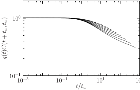
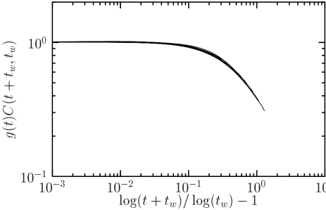
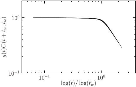
Figure 14: Spin autocorrelation functions at $T=0.04$ rescaled using $t/t_{w}$, $\log(t+t_{w})/\log(t_{w})$ or $\log(t)/\log(t_{w})$ as scaling variables for the aging part (from top to bottom). We only display the 12 largest waiting times, i.e. $t_{w}\in[139,57797]$.

An increasing $\mu$ when temperature is decreased can be rationalized as follows. It is convenient to define an effective relaxation time review1_1 ; BB by $h(t_{w})/h^{\prime}(t_{w})$, see Eq. (23). When $h(t)\sim\log(t)$ this becomes $t_{w}\log(t_{w})$, which is greater than $t_{w}$, leading to an effective superaging behavior since the effective relaxation time grows faster than $t_{w}$. The conclusion is that a crossover towards activated behavior at low $T$ naturally implies an apparent superaging behavior well consistent with our numerics. This argument was already used in Ref. BB, to interpret data in the four dimensional Ising spin glass.

A purely activated behavior together with a simple scaling of the aging part of the decorrelation would imply that the use of $\log(t+t_{w})/\log(t_{w})$ can rescale the data at large times fh . We test this idea in the middle frame in Fig. 14. A comparison with the top frame where $t/t_{w}$ is used shows that a logarithmic rescaling of the data is much better at large times. To our knowledge, this is the first time that a pure logarithmic rescaling of two-time quantities has successfully been employed in a spin glass simulation. This result is important because one of the salient predictions of the scaling approach to spin glasses is the prediction of activated dynamics and logarithmic scaling in the aging regime of finite dimensional spin glasses fh . Experimentally, a logarithmic rescaling of the thermo-remanent magnetization does not collapse the data prep ; these . It does, however, rescale data for the out-of-phase susceptibility at different frequencies $\omega$ yosh4 ; these , but in a much more restricted time regime, $\omega t_{w}\gg 1$.

Theoretical insights are also provided by the exact solution of the non-equilibrium dynamics of mean-field spin glasses which has revealed the existence of dynamic ultrametricity cuku1 ; cuku2 ; BBK . Physically, ultrametricity implies the existence of a broad distribution of relaxation times organized in a hierarchical manner, in the very precise sense described in Ref. cuku1, . Technically, this generalizes Eq. (23) to a continuum of scaling functions $C_{\rm aging}$ associated with a continuum of functions $h(t)$. Interestingly, dynamic ultrametricity also arises in another mean-field solvable model which has the advantage that an exact form for the time decay can be worked out eric . There it was found that two-time correlators scale with the variable $\log(t)/\log(t_{w})$. This is subtly different from the logarithmic rescaling used above but the two scaling variables are not compatible, and only the latter leads to dynamic ultrametricity. We have applied this alternative rescaling in the lower frame in Fig. 14, which shows that it is marginally superior to the logarithmic rescaling used above. Note however that this alternative scaling variable “compresses” slightly more the numerical data, so that we regard both scalings as being of equally good quality. Note too that they are both compatible, in a restricted time window, with an effective description in terms of a superaging behavior. This is again the first time, to our knowledge, that aging data so directly hint at the possible existence of dynamic ultrametricity in a three-dimensional spin glass.

V Summary and conclusion

We have performed the first large scale numerical simulations of the the aging dynamics of the three-dimensional Heisenberg spin glass. We have measured and discussed in detail the behavior of several space-time correlators related both to spin and chiral degrees of freedom. We now summarize our main results.

We find that the non-equilibrium dynamics of spins and chiralities are qualitatively very similar in the range $T\in[0.02,0.16]$ that we have investigated in detail. Two-time autocorrelation functions show the existence of non-zero Edwards-Anderson parameters for spins and chiralities, and the large time behavior is qualitatively similar and exhibit aging behavior, $C(t+t_{w},t_{w})\neq C(t)$, indicating the simultaneous freezing of both spins and chiralities in this temperature window.

Appropriate spatial correlation functions show that aging is due to the development with time of a spin dynamical correlation length, so that aging in spin glasses can be thought of as a sort of coarsening, as proposed long ago by Fisher and Huse fh . All our results are consistent with the growth with time of a random ordering of the spins imposed by the quenched disorder. The chiralities naturally follow the spins but display weaker correlations. This is because spins correlations fall off with power of distance in the non-equilibrium regime, so that the correlations of the chiralities, each of which involves three spins, probably fall off with a faster power law.

The system’s behavior can be simply accounted for without invoking any decoupling between spins and chiralities, and we have explicitly shown that some of the numerical evidence apparently supporting such a decoupling suffers from strong finite size effects.

We find that the growth law of the spin dynamical correlation length changes from a critical power law regime for temperatures close to $T_{c}$ to a slower activated regime at lower temperatures. This crossover naturally influences the scaling behavior of two-time quantities, and we have found evidence that the low temperature behavior of two-time autocorrelations is more naturally interpreted in terms of logarithmic rescalings than the standard $t/t_{w}$ scaling commonly used. In particular, predictions from both droplet or mean-field approaches to spin glass dynamics are equally able to rationalize the time scaling of dynamical functions.

Although qualitatively similar at first sight, we have found that the Heisenberg Edwards-Anderson model in three dimensions behaves quantitatively differently from its Ising cousin in several ways:

1. The Heisenberg model clearly displays an Edwards-Anderson parameter in the dynamics, see Eq. (6) and Fig. 2, whereas the Ising model does not.

2. The growth of the coherence length is not described by a power law but exhibits a rapid crossover towards activated dynamics, see Figs. 11 and 12.

3. Crossover to activated dynamics is also observed in the scaling of two-time quantities which are not described by $t/t_{w}$ scaling in the low temperature phase, see Fig. 14,

4. Much larger length scales are involved in the dynamics at large times and low temperatures, due to the smaller value of the product $z\nu$ of critical exponents, see Eq. (22).

Interestingly, the features listed above that distinguish the Heisenberg from the Ising Edwards-Anderson model also make the aging dynamics of the Heisenberg model much closer to the experimental situation where results are generally more naturally interpreted in terms of thermally activated dynamics and logarithmically slow relaxations review1 ; review1_1 . As far as simple aging protocols are concerned, we have clearly established that aging behavior has to be interpreted in terms of the slow growth with time of a spin glass dynamic correlation length which then dictates scaling behavior of physical properties. Although direct experimental access to $\ell(t_{w})$ is hard orbach , recent comparative studies bert of Ising and Heisenberg samples are in full agreement with our findings that Ising samples display faster growth of a smaller dynamic correlation length on the time scales of interest, see Fig. 12. However, despite these similarities, we have noted that the logarithmic scalings found in this work at low temperatures and large times are not necessarily observed in experiments because of the finite cooling rates used in experiments BB ; cool . Finally, our observation that the Heisenberg model, as opposed to the Ising version, displays a clear crossover towards activated dynamics is in qualitative agreement with a series of recent studies dupuis ; yosh3 ; bert showing that memory effects and the influence of temperature shifts are much stronger in Heisenberg samples.

These conclusions, as well as our preliminary results prep , point to the correctness of the initial intuition which motivated this work that the present model is better-suited to study and understand from a microscopic viewpoint also more complex thermal protocols leading to further non-equilibrium effects.

- (1) K. Binder and A.P. Young, Rev. Mod. Phys. 58, 801 (1986).
- (2) M. Mézard, G. Parisi and M.A. Virasoro, Spin glass theory and beyond (World Scientific, Singapore, 1987).
- (3) E. Marinari, G. Parisi, and J.J. Ruiz-Lorenzo, in Spin glasses and random fields, Ed.: A.P. Young (World Scientific, Singapore, 1998).
- (4) E. Vincent, J. Hamman, M. Ocio, J.-P. Bouchaud, and L.F. Cugliandolo, in Complex behavior of glassy systems, Ed.: M. Rubi (Springer Verlag, Berlin, 1997).
- (5) P. Nordblad and P. Svendlidh, in Spin glasses and random fields, Ed.: A.P. Young (World Scientific, Singapore, 1998).
- (6) J.-P. Bouchaud, L.F. Cugliandolo, J. Kurchan, and M. Mézard, in Spin glasses and random fields, Ed.: A.P. Young (World Scientific, Singapore, 1998).
- (7) L. Berthier, V. Viasnoff, O. White, V. Orlyanchik, and F. Krzakala, in Slow relaxation and non equilibrium dynamics in condensed matter, Eds: J.-L. Barrat, J. Dalibard, M. Feigelman, J. Kurchan (Springer, Berlin, 2003).
- (8) D.S. Fisher and D. A. Huse, Phys. Rev. Lett. 56, 1601 (1986); Phys. Rev. B 38, 373 (1988); ibid. 38, 386 (1988).
- (9) J.-P. Bouchaud, in Soft and fragile matter: non equilibrium dynamics, metastability and flow, Eds.: M.E. Cates and M.R. Evans (Institute of Physics Publishing, Bristol, 2000).
- (10) J.-P. Bouchaud, V. Dupuis, J. Hammann, and E. Vincent, Phys. Rev. B 65, 024439 (2001).
- (11) H. Yoshino, A. Lemaître, and J.-P. Bouchaud, Eur. Phys. J. B 20, 367 (2001).
- (12) L. Berthier and P.C.W. Holdsworth, Europhys. Lett. 58, 35 (2002).
- (13) F. Scheffler, H. Yoshino, and P. Maas, Phys. Rev. B 68, 060404 (2003).
- (14) H. Yoshino, J. Phys. A 36, 10819 (2003).
- (15) A. Barrat and L. Berthier, Phys. Rev. Lett. 87, 087204 (2001).
- (16) L. Berthier, J. Phys. A 36, 10667 (2003).
- (17) J. Kisker, L. Santen, M. Schreckenberg, and H. Rieger, Phys. Rev. B 53, 6418 (1996).
- (18) T. Komori, H. Yoshino, and H. Takayama, J. Phys. Soc. Jpn 68, 3387 (1999); 69, 1192 (2000); 69, Suppl. A 228 (2000).
- (19) L. Berthier and J.-P. Bouchaud, Phys. Rev. B 66, 054404 (2002); Phys. Rev. Lett. 90, 059701 (2003).
- (20) V. Dupuis, E. Vincent, J.-P. Bouchaud, J. Hammann, A. Ito, and H.A. Katori, Phys. Rev. B 64, 174204 (2001).
- (21) P.E. Jönsson, H. Yoshino, and P. Nordblad, Phys. Rev. Lett. 89, 097201 (2002).
- (22) P.E. Jönsson, R. Mathieu, P. Nordblad, H. Yoshino, H. Aruga Katori, and A. Ito, preprint cond-mat/0307640.
- (23) D. Petit, L. Fruchter, and I.A. Campbell, Phys. Rev. Lett. 88, 207206 (2002).
- (24) A preliminary account of this work is given in L. Berthier and A.P. Young, J. Phys. C (at press), preprint cond-mat/0310721.
- (25) L. Berthier and A.P. Young (in preparation).
- (26) J. A. Olive, A.P. Young, and D. Sherrington, Phys. Rev. B 34, 6341 (1986).
- (27) J.R. Banavar and M. Cieplak, Phys. Rev. Lett. 48, 832 (1982).
- (28) W.L. McMillan, Phys. Rev. B 31, 342 (1985).
- (29) H. Kawamura, Phys. Rev. Lett. 68, 3785 (1992).
- (30) H. Kawamura, Phys. Rev. Lett. 80, 5421 (1998).
- (31) K. Hukushima and H. Kawamura, Phys. Rev. E 61, R1008 (2000).
- (32) D. Imagawa and H. Kawamura, preprint cond-mat/0310348.
- (33) J. Villain, J. Phys. C 10, 4793 (1977).
- (34) F. Matsubara, T. Shirakura, and S. Endoh, Phys. Rev. B 64, 092412 (2001).
- (35) T. Nakamura and S. Endoh, J. Phys. Soc. Jpn. 64, 2113 (2002).
- (36) F. Matsubara, T. Shirakura, S. Endoh, and S. Takahashi, J. Phys. A 36, 10881 (2003).
- (37) L.W. Lee and A.P. Young, Phys. Rev. Lett. 90, 227203 (2003).
- (38) H.G. Ballesteros, A. Cruz, L.A. Fernandez, V. Martin-Mayor, J. Pech, J.J. Ruiz-Lorenzo, A. Tarancon, P. Tellez, C.L. Ullod, and C. Ungil, Phys. Rev. B 62, 14237 (2000).
- (39) L.C.E. Struik, Physical aging in amorphous polymers and other materials (Elsevier, Houston, 1978).
- (40) D.A. Huse, Phys. Rev. B 43, 8673 (1991).
- (41) E. Marinari, G. Parisi, F. Ricci-Tersenghi, and J.J. Ruiz-Lorenzo, J. Phys. A 33, 2373 (2000).
- (42) C. De Dominicis and I. Kondor, J. Phys. (Paris) Lett. 45, L205 (1984).
- (43) D.S. Fisher, in Slow relaxations and non equilibrium dynamics in condensed matter, Eds: J.-L. Barrat, J. Dalibard, M. Feigelman, J. Kurchan (Springer, Berlin, 2003).
- (44) P.E. Jönsson, H. Yoshino, P. Nordblad, H. Aruga Katori, and A. Ito, Phys. Rev. Lett. 88, 257204 (2002).
- (45) Y.G. Joh, R. Orbach, G.G. Wood, J. Hammann, and E. Vincent, Phys. Rev. Lett. 82, 438 (1999).
- (46) F. Bert, V. Dupuis, E. Vincent, J. Hammann, and J.-P. Bouchaud, preprint cond-mat/0305088.
- (47) M. Sasaki and O. C. Martin, Phys. Rev. Lett. 91, 097201 (2003).
- (48) D. Hérisson and M. Ocio, Phys. Rev. Lett. 88, 257202 (2002).
- (49) L.F. Cugliandolo and J. Kurchan, J. Phys. A 27, 5749 (1994).
- (50) L.F. Cugliandolo and J. Kurchan, Phil. Mag. B 71, 501 (1995).
- (51) V.S. Zotev, G.F. Rodriguez, G.G. Kenning, R. Orbach, E. Vincent, and J. Hammann, Phys. Rev. B 67, 184422 (2003).
- (52) M. Picco, F. Ricci-Tersenghi, F. Ritort, Eur. Phys. J. B 21, 211 (2001).
- (53) S. Jimenez, V. Martin-Mayor, G. Parisi, and A. Tarancon J. Phys. A.36, 10755, (2003).
- (54) J. Kurchan, Phys. Rev. E 66, 017101 (2002).
- (55) H.G. Katzgraber and I.A. Campbell, preprint cond-mat/0310100.
- (56) V. Dupuis, Thèse de l’Université Paris XI (2002).
- (57) L. Berthier, J.-L. Barrat, and J. Kurchan, Phys. Rev. E 63, 016105 (2001).
- (58) E. Bertin and J.-P. Bouchaud, J. Phys. A 35, 3039 (2002).