Orbital and Spin contributions to the $g$-tensors in metal nanoparticles

Abstract

We present a theoretical study of the mesoscopic fluctuations of $g$-tensors in a metal nanoparticle. The calculations were performed using a semi-realistic tight-binding model, which contains both spin and orbital contributions to the $g$-tensors. The results depend on the product of the spin-orbit scattering time $\tau_{\textrm{\small so}}$ and the mean-level spacing $\delta$, but are otherwise weakly affected by the specific shape of a generic nanoparticle. We find that the spin contribution to the $g$-tensors agrees with Random Matrix Theory (RMT) predictions. On the other hand, in the strong spin-orbit coupling limit $\delta\tau_{\textrm{\small so}}/\hbar\to 0$, the orbital contribution depends crucially on the space character of the quasi-particle wavefunctions: it levels off at a small value for states of $d$ character but is strongly enhanced for states of $sp$ character. Our numerical results demonstrate that when orbital coupling to the field is included, RMT predictions overestimate the typical g-factor of orbitals that have dominant d-character. This finding points to a possible source of the puzzling discrepancy between theory and experiment.

I Introduction

The difference in energy between the eigenvalues for the two spin states of an isolated electron in an external magnetic field $B$ is $g_{0}\mu_{\rm B}B$, where $\mu_{\rm B}$ is the Bohr magneton and $g_{0}$ is the so-called $g$-factor for an isolated electron. If we ignore quantum electrodynamical corrections, it follows from the one-particle Dirac equation that $g_{0}=2$. In an infinite crystal in the absence of external magnetic fields, time-reversal symmetry dictates that each electron Bloch state, labeled by $\bf k$, is doubly degenerate (Kramer’s degeneracy), provided that the crystal has inversion symmetryKittel (1987). This degeneracy is lifted by a magnetic field $B\hat{B}$, and the energy difference between the two states can be expressed by means of a symmetric, $3\times 3\$, “$g$-tensor”, ${\cal G}_{\bf k}$Slichter (1963)

$$\Delta\epsilon_{\bf k}=\mu_{\rm B}B\big{(}\hat{B}^{T}{\cal G}_{\bf k}\hat{B}\big{)}^{1/2}\;.$$ (1)

The tensor ${\cal G}_{\bf k}$ is related to the total magnetic moment of the state $\bf k$ (see below)

$$\mu_{\rm B}\langle\vec{\mu}\ \rangle_{\bf k}=\mu_{\rm B}\langle\vec{L}\rangle_{\bf k}+\mu_{\rm B}\langle g_{0}\vec{S}\rangle_{\bf k}\;.$$ (2)

Here $\mu_{\rm B}\vec{L}$ and $\mu_{\rm B}g_{0}\vec{S}$ are the orbital and spin magnetic moments. The brackets $\langle\dots\rangle_{\bf k}$ denote the expectation value in the $\bf k$-state. In the absence of spin-orbit interactions, the orbital angular momentum is quenched, and only the spin magnetic moment contributes to the level splitting. In this case the Kramer doublet is composed of two (opposite) pure spin states and the tensor ${\cal G}_{\bf k}$ is isotropic, $({\cal G}_{\bf k})_{ij}=4\delta_{ij}$. It follows that the $g$-factor for a magnetic field in the $z$ direction, defined as the square root of the tensor element $({\cal G}_{\bf k})_{zz}$, is equal to the free electron $g_{0}$. The effect of spin-orbit coupling is fourfold: (i) because the states forming a Kramer doublet are no longer pure spin states, their average spin is less than $1/2$, which tends to decrease the typical $g$-factor; (ii) the orbital angular momentum is no longer quenched and the corresponding magnetic moment can contribute to the level splitting, either by decreasing or increasing $g$; (iii) the tensor structure of ${\cal G}$ is non-trivial (i.e. the response to a magnetic field is anisotropic and does not in general lead a moment aligned with the field); (iv) ${\cal G}_{\bf k}$ can vary strongly with ${\bf k}$. In bulk metals direct measurement of electron $g$-factors can be obtained only via conduction electron spin resonance (CESR) experiments. CESR involves transitions between states of the electron continuum. The two quantities measured in these experiments are the position of a resonance line, that is the average $g$-factor of the conduction electrons, over the Fermi surface, $g_{\rm av}$, and the linewidth, corresponding to the spin relaxation time $\tau_{\textrm{\small so}}$. In case of weak spin-orbit interaction the $g$-factor shift $\Delta g\equiv g_{\rm av}-g_{0}$ can be evaluatedElliott (1954) perturbatively in the spin-orbit coupling constant $\xi$, $\Delta g\sim\xi/W$, where $W$ is the band width. Since $W>>\xi$, the effect of spin-orbit interaction on bulk $g$-factors is expected to be small, even for heavy elements like gold. Indeed experimentally $g_{\rm av}$ in Al is essentially equal to $g_{0}$, while for Au $g_{\rm av}=2.1$. When evaluated perturbatively, the spin relaxation time $\tau_{\textrm{\small so}}$ can be related to $\Delta g$ and to the “resistivity” relaxation time $\tau_{r}$ through the Elliott relationElliott (1954), ${1\over\tau_{\textrm{\small so}}}={\Delta g^{2}\over\tau_{r}}$. This relation shows that scattering off impurities, surfaces, and phonons, which determine $\tau_{r}$, affects indirectly $\tau_{\textrm{\small so}}$, although the mechanism responsible for the spin relaxation is the spin-orbit interaction, which is essentially atomic in character.

In this paper we focus on the $g$-factors for electrons confined inside a metal grain of nanometer size, where the quantum energy spectrum is discrete and its individual quasiparticle energy levels $\epsilon_{n}$ can be directly observed at low temperatures. By replacing the Bloch index $\bf k$ with the discrete quasiparticle orbital index $n$, equations (1) and (2) describe how a Kramer doublet splits in a magnetic field. In contrast to the bulk case, the effects on the spin-orbit interaction on $g$ – summarized in (i)-(iv) above – is expected to be enhanced, since the relevant energy scale with which the spin-orbit coupling strength $\xi$ should be compared is not $W$ but the much smaller single-particle mean-level spacing $\delta$. In fact quantum finite-size effects on $g$-factors in ensembles of metal nanoparticles have been investigated in the past experimentally via CESR. (For a review see Ref. Halperin, 1986 and references therein.) To the best of our knowledge though, these experiments are riddled with many puzzling features, which make their comparison with proposed theoriesKawabata (1970); Buttet et al. (1982) very difficult. Furthermore in none of these experiments is there sufficient detail to extract information concerning statistical distribution of $g$-factors (see point (iii) above ). On the other hand, two groupsSalinas et al. (1999); Davidovic and Tinkham (2000); Petta and Ralph (2001, 2002), using tunneling spectroscopy in single-electron transistors, have recently succeeded in measuring $g$-factors of individual quasiparticle levels of a single metal nanoparticle. Measured $g$-factors ranged from 0.1 to 2, depending on material, grain size and doping; $g$-factors displayed large level-to-level fluctuations and strong dependence on the orientation of the applied magnetic field. Clearly $g$-factors in small metal grains measured by single-electron spectroscopy have little in common with bulk $g$-factors measured by CESR.

The statistical properties and mesoscopic fluctuations of $g$-factors measured experimentally in Refs. Salinas et al., 1999; Davidovic and Tinkham, 2000; Petta and Ralph, 2001, 2002 are well described by theoretical distributions based on Random Matrix Theory (RMT), derived by two independent groupsBrouwer et al. (2000); Matveev et al. (2000); Adam et al. (2002). There is however a longstanding puzzle in the comparison between this theory and experiment. The $g$-tensor distributions obtained from RMT are normalized to the average $(\langle g^{2}\rangle)^{1/2}$, which has to be evaluated by independent arguments. In the regime of strong spin-orbit interaction, the two theoretical modelsMatveev et al. (2000); Adam et al. (2002) predict $\langle g^{2}\rangle$ to have contributions from both spin and orbital magnetic moments

$$\langle g^{2}\rangle={3\over\pi\hbar}\tau_{\textrm{\small so}}\delta+\alpha{l\over R}\;,$$ (3)

where $l$ is the elastic mean free path, $R$ is the size of the particle and $\alpha$ is a constant of order 1. In the limit of strong spin-orbit scattering $\tau_{\textrm{\small so}}\delta\to 0$, the spin contribution vanishes and only the orbital contribution $\alpha(l/R)\sim(\langle L_{z}\rangle)^{2}$ survives. The nanoparticles studied in Refs. Petta and Ralph, 2001, 2002 are not disordered and therefore $l\sim R$. Thus Eq. (3) predicts that $\langle g^{2}\rangle$ should never be much less than 1. In noble-metal nanoparticles, however, the measured values of $\langle g^{2}\rangle$ are typically between 0.05 and 0.1.

RMT is a phenomenological approach which assumes that the statistical properties of interest depend only on the symmetry of the Hamiltonian. This assumption, although appealing and reasonable, is usually difficult to justifies rigorously. This fact, together with the discrepancy between theoryMatveev et al. (2000); Adam et al. (2002) and experiment mentioned above, motivates the theoretical study of $g$-factors in metal nanoparticles presented here. Our investigation is based on a semi-realistic microscopic tight-binding model that we solve numerically.

From the comparison between RMT and our microscopic theory we are able to shed some light on the discrepancy between the experimental measurements of $\langle g^{2}\rangle$ and the value predicted in Refs. Matveev et al., 2000; Adam et al., 2002. The results of our model are in agreement with most of the RMT conclusions as to the functional form of the $g$-tensor distribution and its dependence on the spin-orbit coupling strength. In particular we find that $g$-tensors are strongly anisotropic when the nanoparticle shape is not perfectly symmetric, and that this anisotropy originates from mesoscopic quantum fluctuations of the nanoparticle wavefunctions. However, we are able to go beyond RMT, in that our more detailed analysis allows us to clarify the role played by the orbital motion and demonstrate that its contribution to the average $g$-factor is very sensitive to the character of the quasiparticle wavefunctions. Based on these results we conclude that the small value of $\langle g^{2}\rangle$ measured experimentally can be understood if the orbital angular momentum of the tunneling states, in contrast to the RMT assumptions, is still partially quenched.

The paper is organized as follows. In Sec. II we introduce and discuss our model, with particular emphasis on the coupling between orbital motion and external field. In Sec. III we illustrate our numerical results, we compare them with RMT predictions, and we discuss their implications for the interpretation of the tunneling spectroscopy experiments. A summary and concluding remarks are presented in Sec. IV.

II Model

We model the nano-particle as a truncated fcc crystal lattice with $N_{a}$ atoms. The shape of the system can be arbitrarily varied to simulate the variability of realistic nanoparticles. A $spd$ tight-binding-model is used with 18 orbitals at each atomic site, including the spin degrees of freedom.

The Hamiltonian,

$${\cal H}={\cal H}_{\rm band}+{\cal H}_{\textrm{\small so}}+{\cal H}_{\rm Zee},$$ (4)

has been introduced in a study of the quasiparticle properties in ferromagnetic metal nanoparticlesCehovin et al. (2002). Here we give only a brief description of the terms in Eq.(4).

The first term $H_{\rm band}$ is an orbital part,

$${\cal H}_{\rm band}=\sum_{i,j}\sum_{s}\sum_{\mu_{1},\mu_{2}}t^{i,j}_{\mu_{1},\mu_{2},s}c^{\dagger}_{i,\mu_{1},s}c^{\phantom{\dagger}}_{j,\mu_{2},s}$$ (5)

involving the Slater-Koster parameters Slater and Koster (1954), $t^{i,j}_{\mu_{1},\mu_{2},s}$. Atomic sites are labeled by $i,j$, and $t^{i,j}$ couples up to second nearest-neighbors. The indices $\mu_{1},\mu_{2}$ label the nine distinct atomic orbitals (one $4s$, three $4p$ and five $3d$). The spin degrees of freedom, labeled by the index $s$, double the number of orbitals at each site.

The second term describes a spin-orbit interaction, essentially atomic in character

$${\cal H}_{\textrm{\small so}}=\xi\sum_{i}\sum_{\mu,\mu^{\prime},s,s^{\prime}}\langle i,\mu,s|{\vec{L}}\cdot{\vec{S}}|i,\mu^{\prime},s^{\prime}\rangle c^{\dagger}_{i,\mu,s}c^{\phantom{\dagger}}_{i,\mu^{\prime},s^{\prime}},$$ (6)

reflecting the fact that relativistic effects are important only when the electron is close to the nucleus. In spite of the local nature of these interaction, the effect of ${\cal H}_{\textrm{\small so}}$ on the spin-orbit relaxation time $\tau_{\textrm{\small so}}$, compared to non-disordered infinite systems, is strongly enhanced by the destruction of crystal symmetry due to the nanoparticle surface. This is, to a certain extent, similar to the mechanism described by the Elliott relation.

A quantitative measure of the relative strength of the spin-orbit interaction is given by the dimensionless parameter $\lambda$Brouwer et al. (2000)

$$\lambda^{2}=\pi\frac{\hbar}{\tau_{\textrm{\small so}}\delta}\;.$$ (7)

The spin-orbit scattering is strong if $\lambda>>1$ and weak if $\lambda<<1$. In the limit of weak spin-orbit interaction $\tau_{\textrm{\small so}}$ can be calculated perturbatively by Fermi golden rule. Here, however, we use a more pragmatic approach: we define $\tau_{\textrm{\small so}}$ in terms of the average spin-orbit quasiparticle energy shiftCehovin et al. (2002)

$$\hbar\tau^{-1}_{\textrm{\small so}}\equiv\langle|\epsilon_{n}-\epsilon_{n}^{0}|\rangle,$$ (8)

where $\epsilon_{n}$ and $\epsilon_{n}^{0}$ is the $n$-th eigenvalue with and without spin-orbit interaction respectively and the average $\langle\dots\rangle$ is performed over the spectrum of the nanoparticle.

Since $\tau_{\textrm{\small so}}$ decreases weakly with particle size $L$, while $\delta$ varies as ${L}^{-3}$, the effective strength of the spin-orbit interaction decreases with decreasing particle size. In the experiments of Ref. Petta and Ralph, 2001, 2002, containing up to several thousand atoms, $\lambda$ can be as large as $10$ for Au nanoparticles. In our theoretical studies we are able to deal numerically with nanoparticles containing only up to a few hundred atoms, which would yield $\lambda<<1$ for a realistic value of $\xi\approx 100$ meV. In order to achieve larger $\lambda$ values we therefore artificially increase the spin-orbit coupling strength $\xi$. For a disordered dot of a generic shape our numerical results depend on the value of $\lambda$ but only weakly on the separate values of $\xi$ and $\delta$.

The Zeeman part ${\cal H}_{\rm Zee}$ in Eq. (4) is conveniently divided into two terms,

$${\cal H}_{\rm Zee}=-\mu_{\rm B}\sum_{i}\vec{B}\cdot\Big{\{}\sum_{\mu,\mu^{\prime},s,s^{\prime}}\langle i,\mu,s|g_{s}\vec{S}+\vec{L}|i,\mu^{\prime},s^{\prime}\rangle c^{\dagger}_{i,\mu,s}c^{\phantom{\dagger}}_{i,\mu^{\prime},s^{\prime}}\Big{\}}+{\cal H}^{\rm NLOC}_{\rm Zee}$$ (9)

The first term of Eq. (9) is the usual atomic contribution already considered in our earlier paper Cehovin et al. (2002), arising from the space dependence of the vector potential on an atomic length scale. In addition to this, there is a second term, a non-local orbital contribution arising from the magnetic flux encompassed by closed loops describing the paths of an electron hopping from site to site. Only the latter term is accounted for in the RMT approach, whereas the former term has a larger importance in many respects. We discuss this contribution in detail in the next section.

II.1 Non-Local Orbital Contribution (NLOC)

The NLOC originates from delocalized electrons in an external magnetic field. The coupling to an external magnetic field in tight-binding theory is accomplished by the introduction of the Peierls phases Peierls (1933); Luttinger (1951); Graf and Vogl (1995),

$$\exp(i\Theta_{i,j})=\exp\biggl{[}\frac{ie}{\hbar c}\int_{\vec{R}_{i}}^{\vec{R}_{j}}\vec{A}(x)\cdot d\vec{x}\biggr{]}\approx\exp\biggl{[}\frac{ie}{\hbar c}\frac{(\vec{R}_{j}-\vec{R}_{i})\cdot(\vec{A}(\vec{R}_{j})+\vec{A}(\vec{R}_{i}))}{2}\biggr{]},$$ (10)

modifying the Slater-Koster parameters so that,

$${\cal H}^{\rm NLOC}_{\rm Zee}=\sum_{i,j}\sum_{s}\sum_{\mu_{1},\mu_{2}}(\exp(i\Theta_{i,j})-1)t^{i,j}_{\mu_{1},\mu_{2},s}c^{\dagger}_{i,\mu_{1},s}c^{\phantom{\dagger}}_{j,\mu_{2},s}.$$ (11)

The non-trivial approximation of Eq. (10), replacing the contour integral with a simple line integral has been justified by Ismail-Beigi et al. Ismail-Beigi et al. (2001).

Choosing the vector potential in the symmetric gauge,

$$\vec{A}=-\frac{1}{2}\vec{r}\times\vec{B},$$ (12)

the Peierls phases can be conveniently rewritten in a form suitable for perturbation theory purposes,

$$\Theta_{i,j}=-\frac{2\pi}{4\phi_{0}}\big{[}(\vec{R}_{j}-\vec{R}_{i})\times(\vec{R}_{i}+\vec{R}_{j})\big{]}\cdot\vec{B}.$$ (13)

The phase factor of Eq. (10) is expanded to first order in $\vec{B}$,

$$\exp(i\Theta_{i,j})=1-i\mu_{B}\vec{L}^{NLOC}\cdot\vec{B}+O(B^{2}),$$ (14)

where $\vec{L}^{NLOC}$ is defined as

$$\langle i,\mu,s|\vec{L}^{NLOC}|j,\mu^{\prime},s^{\prime}\rangle=\frac{2\pi}{4\mu_{B}\phi_{0}}\big{[}(\vec{R}_{j}-\vec{R}_{i})\times(\vec{R}_{i}+\vec{R}_{j})\big{]}.$$ (15)

This expansion allows one to write Eq. (9) to first order in (small) $\vec{B}$ in the familiar form

$${\cal H}_{\rm Zee}\approx- \mu_{B} \vec{\mu}\cdot\vec{B}\equiv$$ (16)

$$- \mu_{\rm B} \sum_{i}\Big{\{}\sum_{\mu,\mu^{\prime},s,s^{\prime}}\langle i,\mu,s|g_{s}\vec{S}+\vec{L}|i,\mu^{\prime},s^{\prime}\rangle c^{\dagger}_{i,\mu,s}c^{\phantom{\dagger}}_{i,\mu^{\prime},s^{\prime}}\Big{\}}\cdot\vec{B}$$ (17)

$$- \mu_{\rm B} \sum_{i,j}\Big{\{}\sum_{\mu,\mu^{\prime},s,s^{\prime}}\langle i,\mu,s|\vec{L}^{NLOC}|j,\mu^{\prime},s^{\prime}\rangle c^{\dagger}_{i,\mu,s}c^{\phantom{\dagger}}_{j,\mu^{\prime},s^{\prime}}\Big{\}}\cdot\vec{B}\;.$$ (18)

We have explicitly checked that the Zeeman splitting due to the non-local interaction is gauge invariant in our numerical calculations, although the definition presented above is obviously for a particular gauge choice.

II.2 Wannier states

The basis set, $|j,\mu,s\rangle$, is to be interpreted as a set of Wannier orbitals, extracted Slater and Koster (1954) from bulk properties. The Slater-Koster parameters, $t^{i,j}_{\mu_{1},\mu_{2},s}$, are Hamiltonian matrix elements of $|j,\mu,s\rangle$. Application of $t^{i,j}_{\mu_{1},\mu_{2},s}$ to a nano-particle relies on their transferability, the assumption of local electronic environmental insensitivity to the boundaries of the system. The success of this procedure depends on the nature of the states involved . In noble metals the electronic density of the $sp$-bands is delocalized, and very different from a simple sum of atomic densities. The corresponding Wannier orbitals lose their atomic-like character in this limit, and the transferability is expected to be less robust, since the boundary conditions play an increasingly important role. The orbitals, $|j,\mu,s\rangle$, of $sp$-symmetry will thus have large hopping elements, a property expected to remain the same in any transferable tight-binding treatment of these states. The $d$-orbitals originate from bands of a different nature, with rather localized electronic densities around the atomic sites. The corresponding Wannier orbitals remain atomic-like and hopping parameters are small.

From these arguments it is immediately clear that the contribution from ${\cal H}^{\rm NLOC}_{\rm Zee}$ becomes increasingly important in the limit of extended Wannier states with large hopping parameters.

The eigenstates of this model are in general a mixture of all basis orbitals, $|j,\mu,s\rangle$. An approximate separation of the eigenspectrum into bands of specific symmetries can still be made. For this purpose it is useful to define the projection operators, $P_{s},P_{p}$ and $P_{d}$.

$$P_{s} = \sum_{i}\sum_{s}\sum_{\mu_{s}}|i,\mu_{s},s\rangle\langle i,\mu_{s},s|\;,$$ (19)

$$P_{p} = \sum_{i}\sum_{s}\sum_{\mu_{p}}|i,\mu_{p},s\rangle\langle i,\mu_{p},s|\;,$$ (20)

$$P_{d} = \sum_{i}\sum_{s}\sum_{\mu_{d}}|i,\mu_{d},s\rangle\langle i,\mu_{d},s|\;,$$ (21)

with

$$P_{s}+P_{p}+P_{d}=1\;.$$ (22)

These operators project onto the subspaces of $s$, $p$ or $d$-symmetry. As an example, in Fig. (1) we plot the expectation values of these projection operator in the eigenstates $|n\rangle$ of the Hamiltonian of Eq. (4). The calculations are done for a 143 gold atom nanoparticle with hemispherical shape, from which 5 atoms have been removed to break the rotational symmetry. It is seen that states in the middle of the occupied band have well-defined $d$-character, with the exception of some states around $n=700$, which have mixed $spd$-components and low-energy states, which have mainly $s$-character. High-energy states far above the Fermi level have dominant $p$-character. States around the Fermi level are rather strongly mixed with the $d$-component decreasing sharply with eigenvalue number.

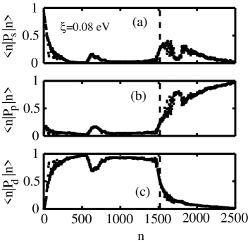
Figure 1: Matrix elements of $P_{\mu}$ according to Eq. (21). The eigenstate $|n>$ is for the Hamiltonian of a 143-atom hemispherical Au nanoparticle, with 5 atoms removed. The dashed vertical line marks the Fermi level.

Data	Material	$<g_{1}>$	$<g_{2}>$	$<g_{3}>$	$\lambda$
Exp.	Cu	$0.9\pm 0.3$	$1.2\pm 0.2$	$1.6\pm 0.3$	$1.1\pm 0.1$
RMT	-	1.0	1.1	1.6	$1.1$
Here	Au	1.1	1.3	1.7	$1.1$
Exp.	Cu	$0.4\pm 0.2$	$0.8\pm 0.2$	$1.3\pm 0.3$	$1.8\pm 0.1$
RMT	-	0.5	0.8	1.3	$1.8$
Here	Au	0.7	0.9	1.4	$1.8$

Table 1: Calculated mean values of $g_{i}$ compared to random matrix theory predictions and experiments. The $g$-factors of our model are based on d-states only. The experimental and random matrix theory data are from Petta and Ralph Petta and Ralph (2002).

II.3 $g$-tensor

In the absence of an external magnetic field, a nano-particle will have a doubly degenerate eigenspectrum, $\epsilon_{n}$, reflecting the formation of Kramer pairs in a time-reversal symmetric system. In the presence of spin-orbit interaction, the Zeeman splittings, $\epsilon_{n}\rightarrow\epsilon_{n}\pm\delta\epsilon_{n}$, show anisotropic dependence on the direction of the applied field, $\vec{B}$. For small $\vec{B}$ this is conveniently described in terms of the $g$-tensor Slichter (1963),

$$\delta\epsilon^{2}_{n}(\vec{B}) = \big{(}\frac{\mu_{B}}{2}\big{)}^{2}\vec{B}\cdot{\cal G}_{n}\cdot\vec{B}$$ (23)

$${\cal G}_{n} = G^{T}_{n}G_{n}.$$ (24)

By using standard degenerate perturbation theory in ${\cal H}_{\rm Zee}$, the $G_{n}$ matrices can be related to the matrix elements of the (dimensionless) magnetic moment operator $\vec{\mu}$,

$$(G_{n})_{1,j}+i(G_{n})_{2,j} = -2\langle T\psi_{n}|\mu_{j}|\psi_{n}\rangle$$ (25)

$$(G_{n})_{3,j} = 2\langle\psi_{n}|\mu_{j}|\psi_{n}\rangle\;.$$ (26)

Here $|\psi_{n}\rangle$ and $|T\psi_{n}\rangle$ are the time-reversed pair of eigenstates of ${\cal H}$ in the absence of $\vec{B}$, corresponding to the eigenvalue $\epsilon^{2}_{n}$. The diagonalization of ${\cal G}_{n}$, or in other words a suitable choice of coordinate system for the external field $\vec{B}$, allows one to write $\delta\epsilon_{n}(\vec{B})$ in terms of the 3 eigenvalues $g_{j}^{2}$, $j=1,2,3$, of ${\cal G}$

$$\delta\epsilon_{n}(\vec{B})=\frac{\mu_{B}}{2}\sqrt{g_{1}^{2}B_{1}^{2}+g_{2}^{2}B_{2}^{2}+g_{3}^{2}B_{3}^{2}},$$ (27)

where $B_{j}$, $j=1,2,3$, are the components of the magnetic field along the “principal axis”, $\hat{e}_{1},\hat{e}_{2},\hat{e}_{3}$, defined by the three normalized eigenstates of ${\cal G}$. We refer to $g_{j},j=1,2,3$ as the principal $g$-factorsBrouwer et al. (2000). The Zeeman splittings, $\delta\epsilon_{n}(\vec{B})$, can also be obtained from direct numerical diagonalization of the Hamiltonian for a given direction of $\vec{B}$. This approach is of course time demanding, but served as a check of the correctness of the perturbative approach, since the two methods should give identical results for small $\vec{B}$.

In the limit of zero spin-orbit interactions the three principal $g$-factors are identically equal to 2. In this case the Kramer pairs are pure spin states and the angular momentum is quenched. With the introduction of spin-orbit interaction spin characters mix, and non-zero orbital contributions Kravtsov and Zirnbauer (1992) to $g_{i}$ are expected. At weak spin orbit strength the spin character mixing is weak and the orbital contribution to $g_{i}$ is small. For large $\lambda$ the spin character mixing is strong, while orbital contributions are expected to increase.

III Results and Discussion

In this section we present results of numerical calculations of $g$-tensors for $Au$-nanoparticles containing 143 atoms. Similar results, not shown here, were obtained for larger and smaller sizes. We first consider the distribution of principal-axis directions. Fig.(2a) shows calculated principal axis directions for a perfect hemisphere. The direction of $\hat{e}_{i}$ is strongly dependent on the symmetry of the nanoparticle, with one axis always along the normal of the base plane. Due to the crystal fcc symmetry and the hemispherical truncation, the two remaining $g$-factors will be degenerate and two principal axes can be arbitrarily chosen within the base plane. This is shown in Fig.(2a), where we plot the direction of the principal axis directions on the unit sphere for all the quasiparticle orbitals of the nanoparticle. The situation changes dramatically with a small distortion of the shape obtained by removing five atoms from the hemispherical truncation. This slight breaking of the spherical symmetry produces a completely random distribution of principal axis, no longer preferentially aligned along crystalline or shape directions, as clearly seen in Fig. (2b). A random distribution of the principal axis directions was originally predicted by RMTBrouwer et al. (2000). Recent experiments Petta and Ralph (2002) measuring principal $g$-factors find random spatial orientation of the corresponding axis directions, $\hat{e}_{i}$. The measurements were performed on Cu nanoparticles with approximately hemispherical shape. The results demonstrates that small irregularities in the boundaries in an otherwise ordered sample are enough to produce completely randomized directions, exactly as happens in our model.

Figure 2: Principal axis directions on the unit sphere for a 143 atom Au hemisphere in (a). In (b) 5 atoms have been removed from the hemisphere. Each point represents one principal axis direction.

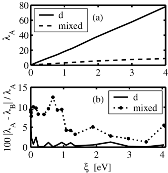
Figure 3: $\lambda_{A}(\xi)$ in (a) shows the spin-orbit strength for a 143-atom Au nanoparticle with 5 atoms removed. $\lambda_{B}(\xi)$ originates from a nanoparticle with a strongly disordered shape, but the same $N_{a}$ as A. The states are divided into $d$-states, $<n|P_{d}|n>>0.7$, and mixed states, $<n|P_{d}|n><0.7$ . (b) shows the differences in $\lambda$ between the two systems in percent.

Once the perfect axial symmetry of the hemispherical nanoparticle is broken, for example by removing a few atoms, we find that the numerical results depend weakly on the particle shape: nanoparticles with shapes that are even less symmetric display qualitatively similar distributions of principal $g$-factors. It turns out that the dimensionless spin-orbit strength $\lambda$, defined in Eqs. (7)-(8), is the crucial parameter that controls the distributions. A meaningful evaluation of $\lambda(\xi)$ for a given value of $\xi$ is however made complicated by the fact that states of different orbital character, as determined by the projection operators discussed above, yield very different values of $\lambda$ for the same $\xi$. Therefore we divide the eigenstates into two groups of states, which we refer to $d$- and mixed states. An eigenstate is operationally considered a $d$-state if $\langle n|P_{d}|n\rangle>0.7$; it is a mixed state otherwise. We will use this distinction extensively below. For a given value of $\xi$, the parameter $\lambda$ is then calculated separately for these two group of states. This procedure turns out to be very useful in the interpretation of our numerical results. A first example of this is shown in Fig. (3). In Fig. (3a) we plot $\lambda(\xi)$ as a function of $\xi$ for these two groups of states for a given nanoparticle. In both cases $\lambda$ increases approximately linearly with $\xi$, but the slope is much larger for the $d$-states. In Fig. (3b) we plot relative differences of the $\lambda$ for two nanoparticles with the same number of atoms ($N_{a}=143$) but very different shapes, again separating $d$- and mixed states. Here $\lambda_{A}$ refers to a nanoparticle with hemispherical shape with 5 atoms removed; $\lambda_{B}$ refers to a nanoparticle with a strongly disordered shape. It is seen that $\lambda$ for the $d$ states is essentially the same for both nanoparticles for all values of $\xi$. On the other hand mixed states give a value of $\lambda$ that is more sensitive on the shape of the nanoparticle, although the relative difference is always less than $10\%$. It follows that the two nanoparticles will have very similar $g$-factor distributions, with a stronger shape dependence of the $g$-factor of mixed character states.

We now come to the discussion of the main results of our paper and to the comparison with RMT predictions. A very useful quantity for this comparison is the average of the sum of the squares of the principal $g$-factors

$$\langle g^{2}\rangle=\frac{1}{3}\langle g_{1}^{2}+g_{2}^{2}+g_{3}^{2}\rangle\;.$$ (28)

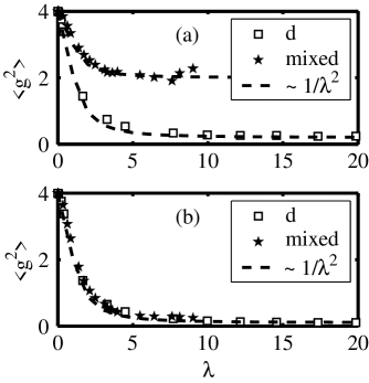
Figure 4: Mean square principal $g$-factors of a 143 atom Au hemisphere with 5 atoms removed. The states are divided into $d$-states, $<n|P_{d}|n>>0.7$ , and mixed states, $<n|P_{d}|n><0.7$ . The full Hamiltonian is used in (a) while the NLOC to the Zeeman term is lacking in (b). The fitting function is given in Eq. (29)

In Fig. 4 we plot $\langle g^{2}\rangle$ as a function of $\lambda$ for a Au hemispherical nanoparticle with 5 atoms removed, separating again the contribution from $d$- and mixed states. The results in Fig. 4(a) are for the case in which the spin term and both orbital terms are included in the magnetic moment of Eq. (2). As expected, $\langle g^{2}\rangle\to 4$ in the limit $\lambda\to 0$ of zero spin-orbit coupling and decreases monotonically with increasing $\lambda$. In the limit of strong spin-orbit coupling, $\lambda>>1$, $\langle g^{2}\rangle$ tends to a constant value, which is relatively small ($\approx 0.3$) for $d$-states but is of order 2 for mixed states. This saturation value in the strong spin-orbit scattering limit comes almost entirely from the non-local orbital contribution (NLOC) to the magnetic moment. Indeed Fig. 4(b) shows that that the saturation value is negligible when the NLOC is not included; in this case the $\langle g^{2}\rangle$ vs. $\lambda$ for $d$- and mixed states fall on the same curve which goes to zero like $1/\lambda^{2}$ for large $\lambda$. Note that the large saturation value for mixed states, when the NLOC is present, is consistent with the fact that $d$-states are linear combination of atomic orbitals with small hopping parameters, whereas mixed states tend to be more free-electron like.

We found that the calculated $\langle g^{2}\rangle(\lambda)$ could always be fit to

$$\langle g^{2}\rangle(\lambda)=\frac{4-\nu(\lambda)}{1+\lambda^{2}}+6\eta^{2}$$ (29)

in the entire range of $\lambda$. Here $\eta$ is a constant independent of $\lambda$, whereas $\nu(\lambda)$ is a function weakly dependent on $\lambda$ such that $\nu(\lambda=0)=6\eta^{2}$ and $\nu(\lambda)\to 1$ for $\lambda>>1$. In practice a reasonable fit (shown in the figure) is obtained by fixing $\nu=6\eta^{2}$. Remembering the relationship between $\lambda$ and $\tau_{\textrm{\small so}}$ given in Eq. (7), we can see that Eq. (29) is perfectly consistent with the RMT predictionMatveev et al. (2000); Adam et al. (2002) in the strong spin-orbit scattering limit given in Eq. (3). The first term in Eq. (29) comes essentially from the spin contribution to the magnetic moment. The second term originates from orbital contributions and it has been written in this specific way to make contact with the the RMT phenomenological parameter $\eta$ that describes its coupling of the magnetic field to the orbital angular momentumAdam et al. (2002). The RMT parameter $\eta^{2}$ can be estimated for specific physical systems by computing $\langle n|L_{z}^{2}|n\rangle$ in the absence of spin-orbit couplingMatveev et al. (2000); Adam et al. (2002). For a ballistic sphere with diffusive boundary conditions one gets $\eta^{2}=1/8$Matveev et al. (2000); Adam et al. (2002). Thus for no disorder RMT predicts for $\langle g^{2}\rangle$ a saturation value $\approx 1$, which according to our model would correspond to the case of mixed states.

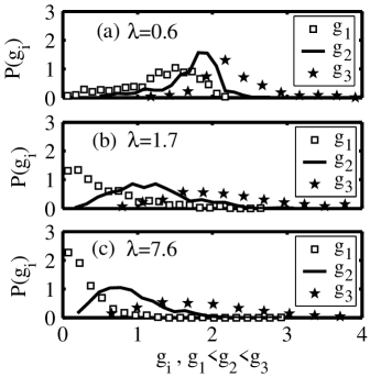
Figure 6: $g$-factor distributions of mixed states for three different values of $\lambda$. The system is a 143 atom Au hemisphere with 5 atoms removed.

We can further analyze the relationship between RMT and our microscopic model by comparing the distribution of the three individual principal $g$-factors in different regimes of the spin-orbit coupling strength. In Fig. 5 and Fig. 6 we plot the distribution of $g_{1}$, $g_{2}$, and $g_{3}$ for $d$ and mixed states respectively. Translating into RMT language, Fig. 5 and Fig. 6 correspond to small and large orbital contribution respectively. The sub-cases (a), (b), (c) in each figure correspond to the regimes of weak, intermediate and strong spin-orbit scattering respectively. The values of $\lambda$ are chosen to compare with the cases considered in Refs. Brouwer et al., 2000; Adam et al., 2002. For weak spin-orbit interaction, we find that typically $g_{1}\approx g_{2}<2$ and $g_{3}\approx 2$ when the spin contribution to the $g$ tensor dominates (i.e. $\eta<<\lambda$ as in Fig.5(a) ). On the other hand, when the orbital contribution dominates the $g$-tensor ($\eta>>\lambda$ as in Fig.6(a) ), $g_{1}<1$, $g_{2}\approx 2$, $g_{3}>2$. Both cases are in remarkable agreement with RMT predictionsBrouwer et al. (2000); Adam et al. (2002)

The trends of our numerical distributions for the cases of intermediate and strong spin-orbit scattering also agree with the RMT scenarioBrouwer et al. (2000). In particular in the strong spin-orbit scattering regime and for weak orbital contribution (see Fig. 5(c) ), all three principal $g$-factors are peaked at values smaller than 0.5. In this case, typical values of $g$ are always much smaller than the free electron value $g_{0}=2$.

We conclude this section by attempting a comparison between the results of our model and the experimental results of Ref. Petta and Ralph, 2002. In Table 1 we have summarized: (i) the experimental measurements of the average values of $g_{i},i=1,2,3$, for two Cu nanoparticles–raws labelled by “Exp”; (ii) the RMT results, including spin contribution only–raws labelled by “RMT”; and (iii) the results of our calculations for $d$-states, including both spin and orbital contributions –raws labelled by “Here”. The procedure to extract these numbers is the following. First the value of $\lambda$ corresponding to a particular nanoparticle is obtainedPetta and Ralph (2002) by matching the RMT value of $\langle g^{2}\rangle$ with the same quantity measured experimentally. Given this $\lambda$, the average values of the principal $g$-factors $\langle g_{1}\rangle$, $\langle g_{2}\rangle$, and $\langle g_{3}\rangle$ can then be calculated theoretically by RMT. This was done in Ref. Petta and Ralph, 2002 and the results are reported in Table I. We can also compute the averages of $g_{i}$ within our microscopic model by choosing the parameter $\xi$ for a given nanoparticle so that the value of $\lambda$ obtained from Eqs. 7-8 is equal to the value extracted from the experiment using RMT. The averages predicted by the two theories (RMT and our macroscopic model) can then be compared with each other and with the values measured experimentally.

From the table one can see that RMT – with orbital contributions neglected – predicts average values of $g_{i}$ in good agreement with the experiments for two different $\lambda$’s corresponding to two different nanoparticles. The message that we want to convey here is that the average $g$ values of $d$-states predicted by our microscopic model, at the same nominal values of $\lambda$ defined through Eqs. 7-8, are also in good agreement with RMT and the experiments, even when the orbital contributions are included. Thus our resuls suggests a scenario, namely $g$-factor distributions of states of mainly $d$ character, which, if realized, would solve the puzzle posed by the comparison between RMT and experiment. Note that RMT is based on a picture of single-particle wavefunctions essentially ergodic in space and it is therefore unable to capture the nature of wavefunctions more localized around atomic cores or defects, which instead are naturally described within our tight binding model.

The problem with the scenario proposed here is that the Fermi level for noble-metal nanoparticles lies near states of both $d$-like and mixed-like character, (see Fig. 1 ) and therefore the latter ones most likely play a very relevant role in the tunneling experiments. However if we use the procedure described above and compute $g$-factor averages including mixed states, we find values that are too large in comparison with experiment.

As possible solutions, we consider the following: (i) electrons are, in fact, tunneling into states of pure $d$ character. (ii) Electrons are tunneling into states of mixed characters, but the nature of these delocalized states is strongly affected by the surface and therefore their characteristics, including their orbital angular momentum, are profoundly modified. This is an effect which is clearly not included in our model, and most likely it is more important for mixed states than for $d$-states. (iii) electron-electron interaction beyond the simple mean-field approximation incorporated in the SK parameters could also modify the electronic states and partially quench their orbital angular momentum. This effect is also not included in our model. Note that recent studiesVoisin et al. (2000) have demonstrated a sharp increase of electron-electron interaction due to surface induced reduction of screening. At the moment we find the occurrence of explanation (i) problematic: apart from the fact that in our calculations all states of pure $d$-character are below the Fermi level and therefore not available for tunneling, states of $s$ character have much larger tunneling probabilities than $d$-states, when (as in the present case) the barriers separating the grain from the electrodes are made of aluminum oxide. Explanations (ii) or (iii) or a combination of the two seem more compelling and alluring. However pursuing these lines requires theoretical modeling beyond the scopes of the present work.

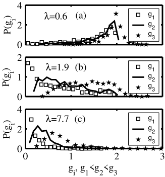
Figure 5: $g$-factor distributions of $d$-states for three different values of $\lambda$. The system is a 143 atom Au hemisphere with 5 atoms removed.

IV Conclusions

In summary, we have presented a theoretical study of the statistical properties of $g$-tensors for individual quasiparticle energy levels of metal nanoparticles, based on numerical calculations for a simplified but realistic model that treats spin-orbit interactions microscopically. Our theory of the $g$-tensors includes both spin and orbital contributions to the magnetic moment. We have shown that even small deviations from a perfectly symmetric nanoparticle shape cause random fluctuations in the quasiparticle wavefunctions, which, in turn, are the source of strong anisotropies of the $g$-tensors and strong level-to-level fluctuations both in the principal $g$-factor values and in the directions of their principal axis. A dimensionless parameter measuring the strength of the spin-coupling controls the $g$-tensor distributions for nanoparticles of generic shape, in excellent agreement with the prediction of random matrix theory. Our work sheds light on the relative importance of the spin vs orbital contributions to the $g$-factors and the strong dependence of the latter on the orbital character of the wave-functions. The presence near the Fermi energy of states of both $d$-like and $sp$-like character is responsible for aspects of the $g$-factor physics that are not captured by Random Matrix Theory. The small values of $g$-factors measured experimentally suggest that the orbital angular momentum of the tunneling states near the Fermi energy is most likely still partially quenched, even in the presence of strong spin-orbit scattering. Our calculations demonstrate that angular momentum quenching cannot be due simply to the strong $d$-orbital hybridization of states near the Fermi energy. Non-trivial changes in electronic structure might be responsible, perhaps due to irregularly shaped nanoparticle boundaries that produce orbitals more localized at the surface than those in the model that we have studied. Enhanced correlation effects near the surface, could also play a role. If surface imperfections are the main source of orbital localization, large $g$-factors should be observable in nanoparticles with very regularly shaped boundaries in which all orbitals are extended across the entire particle.

V Acknowledgments

We would like to thank Dan Ralph for several explanations of his experimental results, and Piet Brouwer, Mandar Deshmukh and Leonid Glazman for stimulating discussions. This work was supported in part by the Swedish Research Council under Grant No:621-2001-2357, by the faculty of natural science of Kalmar University, and in part by the National Science Foundation under Grants DMR 0115947 and DMR 0210383. Support from the Office of Naval Research under Grant N00014-02-1-0813 is also gratefully acknowledged.

References

- Kittel (1987) C. Kittel, Quantum Theory of Solids (John Wiley and Sons, New York, 1987).
- Slichter (1963) C. P. Slichter, Principles of Magnetic Resonance (New York, Evanston, and London, New York, 1963).
- Elliott (1954) R. J. Elliott, Phys. Rev. 96, 266 (1954).
- Halperin (1986) W. P. Halperin, Rev. Mod. Phys. 58, 533 (1986).
- Kawabata (1970) A. Kawabata, J. Phys. Soc. Jpn. 29, 902 (1970).
- Buttet et al. (1982) J. Buttet, R. Car, and C. W. Myles, Phys. Rev. B 26, 2414 (1982).
- Salinas et al. (1999) D. G. Salinas, S. Guéron, D. C. Ralph, C. T. Black, and M. Tinkham, Phys. Rev. B 60, 6137 (1999).
- Davidovic and Tinkham (2000) D. Davidovic and M. Tinkham, Phys. Rev. B 61, R16359 (2000).
- Petta and Ralph (2001) J. R. Petta and D. C. Ralph, Phys. Rev. Lett 87, 266801 (2001).
- Petta and Ralph (2002) J. R. Petta and D. C. Ralph, Phys. Rev. Lett. 89(15), 156802 (2002).
- Brouwer et al. (2000) P. W. Brouwer, X. Waintal, and B. I. Halperin, Phys. Rev. Lett 85, 369 (2000).
- Matveev et al. (2000) K. A. Matveev, L. I. Glazman, and A. I. Larkin, Phys. Rev. Lett 85, 2789 (2000).
- Adam et al. (2002) S. Adam, M. L. Polianski, X. Waintal, and P. W. Brouwer, Phys. Rev. B 66, 195412 (2002).
- Cehovin et al. (2002) A. Cehovin, C. M. Canali, and A. H. MacDonald, Phys. Rev. B 66(10), 094430 (2002).
- Slater and Koster (1954) J. C. Slater and G. F. Koster, Phys. Rev. 94(6), 1498 (1954).
- Peierls (1933) R. Peierls, Z. Phys. 80, 763 (1933).
- Luttinger (1951) J. M. Luttinger, Phys. Rev. B 84, 814 (1951).
- Graf and Vogl (1995) M. Graf and P. Vogl, Phys. Rev. B 51, 4940 (1995).
- Ismail-Beigi et al. (2001) S. Ismail-Beigi, E. K. Chang, and S. G. Louie, Phys. Rev. Lett. 87(8), 087402 (2001).
- Kravtsov and Zirnbauer (1992) V. E. Kravtsov and M. R. Zirnbauer, Phys. Rev. B 46, 4332 (1992).
- Voisin et al. (2000) C. Voisin, D. Christofilos, N. DelFatti, F. Valle, B. Prevel, E. Cottancin, J. Lerme, M. Pellarin, and M. Broyer, Phys. Rev. Lett. 85(10), 2200 (2000).