An extended Hubbard model with ring exchange: a route to a non-Abelian topological phase

Abstract

We propose an extended Hubbard model on a $2D$ Kagomé lattice with an additional ring exchange term. The particles can be either bosons or spinless fermions. At a special filling fraction of $1/6$ the model is analyzed in the lowest non-vanishing order of perturbation theory. Such an “undoped” model is closely related to the Quantum Dimer Model. We show how to arrive at an exactly soluble point whose ground state is the “$d$-isotopy” transition point into a stable phase with a certain type of non-Abelian topological order. Near the “special” values, $d=2\cos\pi/(k+2)$, this topological phase has anyonic excitations closely related to $\text{SU}(2)$ Chern–Simons theory at level $k$.

Since the discovery of the fractional quantum Hall effect in 1982 Tsui et al. (1982), topological phases of electrons have been a subject of great interest. Many Abelian topological phases have been discovered in the context of the quantum Hall regime Das Sarma and Pinczek (1997). More recently, high-temperature superconductivity Anderson (1987); Kivelson et al. (1987); Kalmeyer and Laughlin (1987); Read and Chakraborty (1989); Wen (1991); Mudry and Fradkin (1994); Balents et al. (1998) and other complex materials have provided the impetus for further theoretical studies of and experimental searches for Abelian topological phases. The types of microscopic models admitting such phases are now better understood Moessner and Sondhi (2001); Balents et al. (2002); Senthil and Motrunich (2002).

Much less is known about non-abelian topological phases, apart from some tantalizing hints that the quantum Hall plateau observed at $\nu=5/2$ might correspond to such a non-abelian phase Willett et al. (1987); Moore and Read (1991); Greiter et al. (1992); Nayak and Wilczek (1996). However, non-abelian topological states, if created and controlled, would open the door to scalable quantum computation Kitaev (2003); Freedman (2001). As a first step, the study of a class of topological field theories has been reduced to combinatorial manipulations of loops on a surface Kauffman and Lins (1994); Freedman (2003). A virtue of this formulation is that it exposes a strategy for constructing microscopic physical models which admit the corresponding phases; since Hilbert space is reduced to a set of pictorial rules, the models should impose these rules as energetically favorable conditions satisfied by the ground state. In this paper, we show how this approach can be implemented.

We propose a microscopic model which has the following properties: (a) it is an extension of the Hubbard model and, therefore, is quasi-realistic, (b) it is soluble, (c) for certain model parameters, it is perched at a transition point Freedman et al. (2004a) into a non-Abelian topological phase relevant to quantum computation. By quasi-realistic, we mean that the model has short-ranged interactions and hopping, so it is possible that the Hamiltonian of a real material could be viewed as a small perturbation of the Hamiltonian of this paper. Optical lattices Greiner et al. (2002), quantum dot or Josephson junction arrays Ioffe et al. (2002) might be designed with Hamiltonians in this general class, and these may also be promising avenues for realizing our model.

The non-Abelian topological phases referred to in the above paragraph are related to the doubled $\text{SU}(2)_{k}$ Chern-Simons theories described in Freedman (2003); Freedman et al. (2004b). These phases are characterized by $(k+1)^{2}$-fold ground state degeneracy on the torus $T^{2}$ and should be viewed as a natural family containing the topological (deconfined) phase of $\text{Z}_{2}$ gauge theory as its initial element, $k=1$. For $k\geq 2$ the excitations are non-Abelian. For $k=3$ and $k\geq 5$ the excitations are computationally universal Freedman et al. (2002a). Here, we describe the conditions which a microscopic model should satisfy to be in such a topological phase. It is useful to think of such a microscopic model as a lattice regularization of a continuum model whose low energy Hilbert space may be described as a quantum loop gas. More precisely, a state is defined as a collection of non-intersecting loops, as discussed in Freedman et al. (2004b, 2003b, a). A Hamiltonian acting on such state can do the following: (i) the loops can be continuously deformed – we will call this “move” an isotopy move; (ii) a small loop can be created or annihilated – the combined effect of this move and the isotopy move has been dubbed ‘$d$-isotopy’Freedman (2003); Freedman et al. (2004b, a); (iii) finally, when exactly $k+1$ strands come together in some local neighborhood, the Hamiltonian can cut them and reconnect the resulting “loose ends” pairwise so that the newly-formed loops are still non-intersecting. More specifically, in order for this model to be in a topological phase, the ground state of this Hamiltonian should be a superposition of all such pictures with the additional requirements that (i) if two pictures can be continuously deformed into each other, they enter the ground state superposition with the same weight; (ii) the amplitude of a picture with an additional loop is $d$ times that of a picture without such loop; (iii) this superposition is annihilated by the application of the Jones–Wenzl (JW) projector that acts locally by reconnecting $k+1$ strands. Readers interested in the details are referred to Freedman (2003); Freedman et al. (2004b, 2003b) and references therein. In this paper, we focus on the first two conditions, which place the system at a transition point into the desired phase(s) Freedman et al. (2004a); our purpose is to construct a Hamiltonian which enforces $d$-isotopy for its ground state(s).

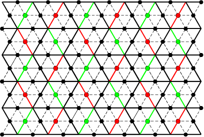
Figure 1: Solid dots and dashed lines represent sites and bonds of the Kagomé lattice $\mathcal{K}$ with the special sublattices $\mathcal{R}$ (red) and $\mathcal{G}$ (green). Solid lines define the surrounding triangular lattice.

Our proposed model is defined on the Kagomé lattice shown in Fig. 1. The sites of the lattice are not completely equivalent, in particular we choose two special sublattices - $\mathcal{R}$ (red) and $\mathcal{G}$ (green) whose significance will be discussed later. The Hamiltonian is given by:

$$H=\sum_{i}\mu_{i}n_{i}+U_{0}\sum_{i}n^{2}_{i}+U\!\!\!\sum_{(i,j)\in\hexagon}\!\!n_{i}n_{j}+\!\!\!\!\sum_{(i,j)\in\bowtie,\notin\hexagon}\!\!\!V_{ij}n_{i}n_{j}\\ -\sum_{\langle i,j\rangle}t_{ij}(c^{\dagger}_{i}c_{j}+c^{\dagger}_{j}c_{i})+T_{\text{R}}.$$ (1)

Here $n_{i}\equiv c_{i}^{\dagger}c_{i}$ is the occupation number on site $i$, $\mu_{i}$ is the corresponding chemical potential. $U_{0}$ is the usual onsite Hubbard energy $U_{0}$ (clearly superfluous for spinless fermions). $U$ is a (positive) Coulomb penalty for having two particles on the same hexagon while $V_{ij}$ represent a penalty for two particles occupying the opposite corners of “bow ties” (in other words, being next-nearest neighbors on one of the straight lines). We allow for the possibility of inhomogeneity so not all $V_{ij}$ are assumed equal. Specifically, define $v^{c}_{ab}=V_{ij}$ where $a$ is the color of site $(i)$, $b$ is the color of $(j)$, and $c$ is the color of the site between them. In the lattice in Fig. 1 we have, possibly distinct, $v^{g}_{bb}$, $v^{b}_{bb}$, $v^{g}_{bg}$, $v^{b}_{rb}$, and $v^{b}_{rg}$, where $r\in\mathcal{R}$, $g\in\mathcal{G}$, and $b\in\mathcal{B}=\mathcal{K}\diagdown(\mathcal{R}\cup\mathcal{G})$. $t_{ij}$ is the usual nearest-neighbor tunnelling amplitude which is also assumed to depend only on the color of the environment: $t_{ij}\equiv t^{c}_{ab}$ where $c$ now refers to the color of the third site in a triangle. Finally, we include $T_{\text{R}}$ – a four-particle ring exchange term whose exact form will be specified later. $T_{\text{R}}$ is added to the Hamiltonian on an ad hoc basis to allow correlated multi-particle hops. Ring exchange terms can be justified semiclassically Roger (1984) and they do indeed appear in in such physical systems as spin systems Herring (1962); MacDonald et al. (1988), solid ³He Thouless (1965) and Wigner crystals Chakravarty et al. (1999). Of course, small ring terms can arise perturbatively along the lines of MacDonald et al. (1988), e.g. a four-particle move occurs at order 4.

The onsite Hubbard energy $U_{0}$ is considered to be the biggest energy in the problem, and we shall set it to infinity, thereby restricting our attention to the low-energy manifold with sites either unoccupied or singly-occupied. The rest of the energies satisfy the following relations: $U\gg t_{ij},V_{ij},\mu_{i}$; we shall be more specific about relations between various $t_{ij}$’s, $V_{ij}$’s and $\mu_{i}$’s later.

The “undoped” system corresponds to the filling fraction 1/6 (i.e. $N_{p}\equiv\sum_{i}n_{i}=N/6$, where $N$ is the number of sites in the lattice). The lowest-energy band then consists of configurations in which there is exactly one particle per hexagon, hence all $U$-terms are set to zero. These states are easier to visualize if we consider a triangular lattice $\mathcal{T}$ whose sites coincide with the centers of hexagons of $\mathcal{K}$. ($\mathcal{K}$ is a surrounding lattice for $\mathcal{T}$.) Then a particle on $\mathcal{K}$ is represented by a dimer on $\mathcal{T}$ connecting the centers of two adjacent hexagons of $\mathcal{K}$. The condition of one particle per hexagon translates into the requirement that no dimers share a site. In the 1/6-filled case this low-energy manifold coincides with the set of all dimer coverings (perfect matchings) of $\mathcal{T}$. The “red” bonds of $\mathcal{T}$ (the ones corresponding to the sites of sublattice $\mathcal{R}$) themselves form one such dimer covering, a so-called “staggered configuration”. This particular covering is special: it contains no “flippable plaquettes”, or rhombi with two opposing sides occupied by dimers (see Fig. 1).

So henceforth particles live on bonds of the triangular lattice (Fig. 1) and are represented as dimers . In particular, a particle hop corresponds to a dimer “pivoting” by $60^{\circ}$ around one of its endpoints, $V_{ij}=v^{c}_{ab}$ is now a potential energy of two parallel dimers on two opposite sides of a rhombus (with $c$ being the color of its short diagonal). It is clear that our model is in the same family as the quantum dimer model Kivelson et al. (1987), which has recently been shown to have an Abelian topological phase on the triangular lattice Moessner and Sondhi (2001) which, corresponds to $k=1$, or $d=1$. Here, we show how other values of $k$ can be obtained.

The goal now is to derive the effective Hamiltonian acting on this low-energy manifold represented by all possible dimer coverings of $\mathcal{T}$. Our analysis is perturbative in ${t}/{U}=:\epsilon$. The initial, unperturbed ground state manifold for $U_{0}=\infty$, $U$ large and positive, all $t_{ij},\;V_{ij}=0$ and all $\mu_{i}$ equal is spanned by the dimerizations $\mathcal{D}$ of the triangular lattice $\mathcal{T}$. As we gradually turn on the $t$’s, $v$’s, and $T_{\text{R}}$, we shall see what equations they should satisfy so that the effective Hamiltonian on $\mathcal{D}$ has the desired $d$-isotopy space as its ground state(s).

Since a single tunnelling event in $\mathcal{D}$ always leads to dimer “collisions” (two dimers sharing an endpoint) with energy penalty $U$, the lowest order at which the tunnelling processes contribute to the effective low-energy Hamiltonian is 2. At this order, the tunnelling term leads to two-dimer “plaquette flips” as well as renormalization of bare onsite potentials $\mu_{i}$’s due to dimers pivoting out of their positions and back. We always recompute bare potentials $\mu_{i}$’s to maintain equality up to errors $\mathcal{O}(\epsilon^{3})$ among the renormalized $\widetilde{\mu}_{i}$’s. This freedom to engineer the chemical potential landscape to balance kinetic energy is essential to finding an exactly soluble point.

Let us pause and discuss the connection between our quantum dimer model and a desired topological phase . It is an old idea (see e.g. Sutherland (1988)) to turn a dimerization (perfect matching) $\mathcal{J}$ into a collection of loops by using a background dimerization $\mathcal{R}$ to form a ‘transition graph’ $\mathcal{R}\cup\mathcal{J}$. It turns out that fixing $\mathcal{R}$ as in Fig. 1, without small rhombi with two opposite sides red, as the preferred background dimerization we obtain the fewest equations in and also achieve ergodicity Kenyon and Rèmila (1996) under a small set of moves. Unlike in the usual case, the background dimerization $\mathcal{R}$ is not merely a guide for the eyes, it is physically distinguished: the chemical potentials and tunnelling amplitudes are different for bonds of different color.

Let us list here the elementary dimer moves that preserve the proper dimer covering condition:
(i) Plaquette (rhombus) flip – this is a two-dimer move around a rhombus made of two lattice triangles. Depending on whether a “red” bond forms a side of such a rhombus, its diagonal, or is not found there at all, the plaquettes are referred to, respectively, as type 1 (or 1’), 2, or 3 (see Fig. 2). The distinction between plaquettes of type 1 and 1’ is purely directional: diagonal bonds in plaquettes of type 1 are horizontal, for type 1’ they are not. This distinction is necessary since our Hamiltonian breaks the rotational symmetry of a triangular (or Kagomé) lattice.
(ii) Triangle move – this is a three-dimer move around a triangle made of four elementary triangles. One such “flippable” triangle is labelled 4 in Fig. 2.
(iii) Bow tie move – this is a four-dimer move around a “bow tie” made of six elementary triangles. One such “flippable” bow tie is labelled 5 in Fig. 2.

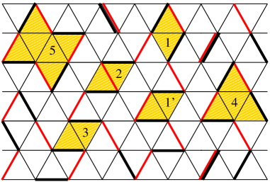
Figure 2: Overlap of a dimer covering of $\mathcal{T}$ (shown in thick black) with the red covering corresponding to the special sublattice $\mathcal{R}$. Shaded plaquettes correspond to various dimer moves described in the text. Green sublattice is not shown.

To make each of the above moves possible, the actual dimers and unoccupied bonds should alternate around a corresponding shape. Notice that for both triangle and bow tie moves we chose to depict the cases when the maximal possible number of “red” bonds participate in their making (2 and 4 respectively). Note that there are no alternating red/black rings of fewer than 8 lattice bonds (occupied by at most 4 non-colliding dimers). Ring moves only occur when red and black dimers alternate; the triangle labelled 4 in Fig. 2 does not have a ring exchange term associated with it, but the bow tie labelled 5 does:

$$T_{\text{R}}=a\;\Bigg{|}\lambda\;\pspicture[-0.05](22.76219pt,19.71262pt)\psset{linewidth=2.0pt}{\psset{linecolor=black}\psline(0.0pt,9.85631pt)(11.38109pt,9.85631pt)}{\psset{linecolor=red}\psline(11.38109pt,9.85631pt)(22.76219pt,9.85631pt)}{\psset{linecolor=black}\psline(22.76219pt,9.85631pt)(17.07164pt,0.0pt)}{\psset{linecolor=red}\psline(17.07164pt,0.0pt)(22.76219pt,-9.85631pt)}{\psset{linecolor=black}\psline(22.76219pt,-9.85631pt)(11.38109pt,-9.85631pt)}{\psset{linecolor=red}\psline(11.38109pt,-9.85631pt)(0.0pt,-9.85631pt)}{\psset{linecolor=black}\psline(0.0pt,-9.85631pt)(5.69054pt,0.0pt)}{\psset{linecolor=red}\psline(5.69054pt,0.0pt)(0.0pt,9.85631pt)}{\psset{linecolor=black,linestyle=dotted,linewidth=1.0pt}\psline(5.69054pt,0.0pt)(17.07164pt,0.0pt)}{\psset{linecolor=black,linestyle=dotted,linewidth=1.0pt}\pspolygon(5.69054pt,0.0pt)(11.38109pt,9.85631pt)(17.07164pt,0.0pt)(11.38109pt,-9.85631pt)}\endpspicture-\pspicture[-0.05](22.76219pt,19.71262pt)\psset{linewidth=1.5pt}{\psset{linecolor=black,linestyle=dotted,linewidth=1.0pt}\psline(0.0pt,9.85631pt)(11.38109pt,9.85631pt)}{\psset{linecolor=red}\psline(11.38109pt,9.85631pt)(22.76219pt,9.85631pt)}{\psset{linecolor=black}\psline(11.38109pt,10.99442pt)(22.76219pt,10.99442pt)}{\psset{linecolor=black,linestyle=dotted,linewidth=1.0pt}\psline(22.76219pt,9.85631pt)(17.07164pt,0.0pt)}{\psset{linecolor=red}\psline(17.07164pt,0.0pt)(22.76219pt,-9.85631pt)}{\psset{linecolor=black}\psline(17.92522pt,0.85358pt)(23.61577pt,-9.00273pt)}{\psset{linecolor=black,linestyle=dotted,linewidth=1.0pt}\psline(22.76219pt,-9.85631pt)(11.38109pt,-9.85631pt)}{\psset{linecolor=red}\psline(11.38109pt,-9.85631pt)(0.0pt,-9.85631pt)}{\psset{linecolor=black}\psline(11.38109pt,-8.7182pt)(0.0pt,-8.7182pt)}{\psset{linecolor=black,linestyle=dotted,linewidth=1.0pt}\psline(0.0pt,-9.85631pt)(5.69054pt,0.0pt)}{\psset{linecolor=red}\psline(5.69054pt,0.0pt)(0.0pt,9.85631pt)}{\psset{linecolor=black}\psline(6.54413pt,0.85358pt)(0.85358pt,10.70988pt)}{\psset{linecolor=black,linestyle=dotted,linewidth=1.0pt}\psline(5.69054pt,0.0pt)(17.07164pt,0.0pt)}{\psset{linecolor=black,linestyle=dotted,linewidth=1.0pt}\pspolygon(5.69054pt,0.0pt)(11.38109pt,9.85631pt)(17.07164pt,0.0pt)(11.38109pt,-9.85631pt)}\endpspicture\Bigg{\rangle}\Bigg{\langle}\lambda\;\pspicture[-0.05](22.76219pt,19.71262pt)\psset{linewidth=2.0pt}{\psset{linecolor=black}\psline(0.0pt,9.85631pt)(11.38109pt,9.85631pt)}{\psset{linecolor=red}\psline(11.38109pt,9.85631pt)(22.76219pt,9.85631pt)}{\psset{linecolor=black}\psline(22.76219pt,9.85631pt)(17.07164pt,0.0pt)}{\psset{linecolor=red}\psline(17.07164pt,0.0pt)(22.76219pt,-9.85631pt)}{\psset{linecolor=black}\psline(22.76219pt,-9.85631pt)(11.38109pt,-9.85631pt)}{\psset{linecolor=red}\psline(11.38109pt,-9.85631pt)(0.0pt,-9.85631pt)}{\psset{linecolor=black}\psline(0.0pt,-9.85631pt)(5.69054pt,0.0pt)}{\psset{linecolor=red}\psline(5.69054pt,0.0pt)(0.0pt,9.85631pt)}{\psset{linecolor=black,linestyle=dotted,linewidth=1.0pt}\psline(5.69054pt,0.0pt)(17.07164pt,0.0pt)}{\psset{linecolor=black,linestyle=dotted,linewidth=1.0pt}\pspolygon(5.69054pt,0.0pt)(11.38109pt,9.85631pt)(17.07164pt,0.0pt)(11.38109pt,-9.85631pt)}\endpspicture-\pspicture[-0.05](22.76219pt,19.71262pt)\psset{linewidth=1.5pt}{\psset{linecolor=black,linestyle=dotted,linewidth=1.0pt}\psline(0.0pt,9.85631pt)(11.38109pt,9.85631pt)}{\psset{linecolor=red}\psline(11.38109pt,9.85631pt)(22.76219pt,9.85631pt)}{\psset{linecolor=black}\psline(11.38109pt,10.99442pt)(22.76219pt,10.99442pt)}{\psset{linecolor=black,linestyle=dotted,linewidth=1.0pt}\psline(22.76219pt,9.85631pt)(17.07164pt,0.0pt)}{\psset{linecolor=red}\psline(17.07164pt,0.0pt)(22.76219pt,-9.85631pt)}{\psset{linecolor=black}\psline(17.92522pt,0.85358pt)(23.61577pt,-9.00273pt)}{\psset{linecolor=black,linestyle=dotted,linewidth=1.0pt}\psline(22.76219pt,-9.85631pt)(11.38109pt,-9.85631pt)}{\psset{linecolor=red}\psline(11.38109pt,-9.85631pt)(0.0pt,-9.85631pt)}{\psset{linecolor=black}\psline(11.38109pt,-8.7182pt)(0.0pt,-8.7182pt)}{\psset{linecolor=black,linestyle=dotted,linewidth=1.0pt}\psline(0.0pt,-9.85631pt)(5.69054pt,0.0pt)}{\psset{linecolor=red}\psline(5.69054pt,0.0pt)(0.0pt,9.85631pt)}{\psset{linecolor=black}\psline(6.54413pt,0.85358pt)(0.85358pt,10.70988pt)}{\psset{linecolor=black,linestyle=dotted,linewidth=1.0pt}\psline(5.69054pt,0.0pt)(17.07164pt,0.0pt)}{\psset{linecolor=black,linestyle=dotted,linewidth=1.0pt}\pspolygon(5.69054pt,0.0pt)(11.38109pt,9.85631pt)(17.07164pt,0.0pt)(11.38109pt,-9.85631pt)}\endpspicture\;\Bigg{|}.$$ (2)

Here is the correspondence between the previous smooth discussion and rhombus flips relating dimerizations $\mathcal{J}$ of $\mathcal{T}$. Our surface is now a planar domain with, possibly, periodic boundary conditions (a torus). A collection of loops is generated by $\mathcal{R}\cup\mathcal{J}$ (with the convention that the dimers of $\mathcal{R}\cap\mathcal{J}$ be consider as length 2 loops or bigons). What about isotopy? Move 2 certainly is an isotopy from $\mathcal{R}\cup\mathcal{J}$ to $\mathcal{R}\cup\mathcal{J}^{\prime}$ but by itself, it does almost nothing. It is impossible to build up large moves from type 2 alone. So it is a peculiarity of the rhombus flips that we have no good analog of isotopy alone but instead go directly to $d-$isotopy. We should impose the following relations associated with moves of type 1 (1’):

$$d\;\Psi\left(\pspicture[0.0](17.07164pt,9.85631pt)\psset{linewidth=2.0pt}{\psset{linecolor=black}\psline(0.0pt,-2.84526pt)(5.69054pt,7.01103pt)}{\psset{linecolor=red}\psline(5.69054pt,7.01103pt)(17.07164pt,7.01103pt)}{\psset{linecolor=black}\psline(17.07164pt,7.01103pt)(11.38109pt,-2.84526pt)}{\psset{linecolor=black,linestyle=dotted,linewidth=1.0pt}\psline(0.0pt,-2.84526pt)(11.38109pt,-2.84526pt)}{\psset{linecolor=black,linestyle=dotted,linewidth=1.0pt}\psline(5.69054pt,7.01103pt)(11.38109pt,-2.84526pt)}\endpspicture\right)-\Psi\left(\pspicture[0.0](17.07164pt,9.85631pt)\psset{linewidth=2.0pt}{\psset{linecolor=black,linestyle=dotted,linewidth=1.0pt}\psline(0.0pt,-2.84526pt)(5.69054pt,7.01103pt)}{\psset{linecolor=red,linewidth=1.5pt}\psline(5.69054pt,7.01103pt)(17.07164pt,7.01103pt)}{\psset{linecolor=black,linewidth=1.5pt}\psline(5.69054pt,8.14914pt)(17.07164pt,8.14914pt)}{\psset{linecolor=black,linestyle=dotted,linewidth=1.0pt}\psline(17.07164pt,7.01103pt)(11.38109pt,-2.84526pt)}{\psset{linecolor=black}\psline(0.0pt,-2.84526pt)(11.38109pt,-2.84526pt)}{\psset{linecolor=black,linestyle=dotted,linewidth=1.0pt}\psline(5.69054pt,7.01103pt)(11.38109pt,-2.84526pt)}\endpspicture\right)=0$$ (3)

since we pass from zero to one loop in (3). Additionally, the ring exchange term (2) annihilates the superposition of one and four loops; we therefore require that $\lambda=d^{3}$.

Having stated our goal, we now derive the effective Hamiltonian $\tilde{H}:\mathcal{D}\to\mathcal{D}$ on the span of dimerizations. The derivation is perturbative to the second order in $\epsilon$ where $\epsilon=t^{r}_{bb}/U=t^{b}_{gb}/U$. Additionally, $t^{b}_{rb}/U=c_{0}\epsilon$ where $c_{0}$ is a positive constant, while $t^{g}_{bb}={o}(\epsilon)$ and can be neglected in the second-order calculations. (In the absence of a magnetic field all $t$’s can be made real and hence symmetric with respect to their lower indices. Also, we set $U=1$ for notational convenience.) We account for all second-order processes, i.e. those processes that take us out of $\mathcal{D}$ and then back to $\mathcal{D}$. These amount to off-diagonal (hopping) processes – “plaquette” flips” or “rhombus moves” – as well as diagonal ones (potential energy) in which a dimer pivots out and then back into its original position. The latter processes lead to renormalization of the bare onsite potentials $\mu_{i}$, which we have adjusted so that all renormalized potentials $\tilde{\mu}_{i}$ are equal up to corrections $\mathcal{O}(\epsilon^{3})$. The non-constant part of the effective Hamiltonian comes from the former processes and can be written in the form: $\tilde{H}=\sum_{\mathcal{I},\mathcal{J}}\left(\tilde{H}_{\mathcal{I}\mathcal{J}}\otimes\mathbb{I}\right)\Delta_{\mathcal{I}\mathcal{J}}$ where $\tilde{H}_{\mathcal{I}\mathcal{J}}$ is a $2\times 2$ matrix corresponding to a dimer move in the two-dimensional basis of dimer configurations connected by this move. $\Delta_{\mathcal{I}\mathcal{J}}=1$ if the dimerizations ${\mathcal{I},\mathcal{J}}\in\mathcal{D}$ are connected by an allowed move, $\Delta_{\mathcal{I}\mathcal{J}}=0$ otherwise. Therefore it suffices to specify these $2\times 2$ matrices $\tilde{H}_{\mathcal{I}\mathcal{J}}$ for the off-diagonal processes. For moves of types (1)–(3), they are given below:

$$\tilde{H}^{(1)}=\begin{pmatrix}v^{b}_{gb}&-2t^{b}_{rb}t^{b}_{gb}\\ -2t^{b}_{rb}t^{b}_{gb}&v^{b}_{rb}\end{pmatrix}=\begin{pmatrix}v^{b}_{gb}&-2c_{0}\epsilon^{2}\\ -2c_{0}\epsilon^{2}&v^{b}_{rb}\end{pmatrix},$$ (4a)

$$\tilde{H}^{(1^{\prime})}=\begin{pmatrix}v^{b}_{bb}&-2t^{b}_{rb}t^{b}_{gb}\\ -2t^{b}_{rb}t^{b}_{gb}&v^{b}_{rg}\end{pmatrix}=\begin{pmatrix}v^{b}_{bb}&-2c_{0}\epsilon^{2}\\ -2c_{0}\epsilon^{2}&v^{b}_{rb}\end{pmatrix},$$ (4b)

$$\tilde{H}^{(2)}=\begin{pmatrix}v^{r}_{bb}&-2(t^{r}_{bb})^{2}\\ -2(t^{r}_{bb})^{2}&v^{r}_{bb}\end{pmatrix}=\begin{pmatrix}v^{r}_{bb}&-2\epsilon^{2}\\ -2\epsilon^{2}&v^{r}_{bb}\end{pmatrix},$$ (4c)

$$\tilde{H}^{(3)}=\begin{pmatrix}v^{g}_{bb}&-2(t^{g}_{bb})^{2}\\ -2(t^{g}_{bb})^{2}&v^{g}_{bb}\end{pmatrix}=\begin{pmatrix}v^{g}_{bb}&0\\ 0&v^{g}_{bb}\end{pmatrix}.$$ (4d)

We can now tune $\tilde{H}$ to the “small loop” value $d$. We require $\tilde{H}^{(1)}=\tilde{H}^{(1^{\prime})}\propto\left(\begin{smallmatrix}d&-1\\ -1&d^{-1}\end{smallmatrix}\right)$ as these moves change the number of small loops by one (cf. Eq. (3)). Since a move of type 2 is just an isotopy move, we require $\tilde{H}^{(2)}\propto\left(\begin{smallmatrix}1&-1\\ -1&1\end{smallmatrix}\right)$. Finally, $\tilde{H}^{(3)}=0$ provided $k>1$, since it represents a “surgery” on two strands not allowed for $k>1$. (For $k=1$, on the other hand, $\tilde{H}^{(3)}\propto\left(\begin{smallmatrix}1&-1\\ -1&1\end{smallmatrix}\right)$.) At level $k=1$ configurations which differ by such a surgery should have equal coefficients in any ground state vector $\Psi$ while at levels $k>1$ no such relation should be imposed. Thus, for $k>1$ the matrix relations (4a-4d) yield equations in the model parameters:

$$\text{Types }(1)\&(1^{\prime}): v^{b}_{gb}=v^{b}_{bb}=2dc_{0}\epsilon^{2}$$ (5a)

$$\text{and}\quad v^{b}_{rb}=v^{b}_{rg}=2d^{-1}c_{0}\epsilon^{2}$$ (5b)

$$\text{Types }(2)\&(3): v^{r}_{bb}=2\epsilon^{2}\quad\text{and}\quad v^{g}_{bb}=0$$ (5c)

We have already assumed that the Hamiltonian has a bare ring exchange term, $T_{\text{R}}$ given by Eq. (2) or, in matrix form, $T_{\text{R}}=a\left(\begin{smallmatrix}\lambda^{2}&-\lambda\\ -\lambda&1\end{smallmatrix}\right)$ where $\lambda=d^{3}$ according to the discussion after Eq. (3). Additionally, we would want the off-diagonal elements of $T_{\text{R}}$, $-a\lambda$ to be of order $\epsilon^{2}$ thus making sure that this ring exchange dominates all other ring exchanges that will appear in the higher orders of perturbation theory. Along with Eqs. (5), these conditions place our model at the soluble point characterized by $d$-isotopy. We remark that additional freedom in defining $T_{\text{R}}$ can be gained by exploiting the the ambiguity of whether a bigon should be considered a loop or not, as discussed in Freedman et al. (2003b). In particular, this allows one to make the diagonal elements of $T_{\text{R}}$ equal.

This construction shows how an extended Hubbard model with an additional ring exchange term (or the equivalent Quantum Dimer Model) can be tuned to the $d$-isotopy state(s). As discussed earlier, they satisfy two of the three conditions which define a class of stable, gapped topological phases which are centered about the special values $d=2\cos(\pi/k+2)$. The next step is to understand how perturbations can push the system (by implementing the JW projectors) into these phases. Our simplest candidate for a “universal quantum computer” is associated with $d=({1+\sqrt{5}})/{2}$.