Vortex line in a neutral finite-temperature superfluid Fermi gas

Abstract

The structure of an isolated vortex in a dilute two-component neutral superfluid Fermi gas is studied within the context of self-consistent Bogoliubov-de Gennes theory. Various thermodynamic properties are calculated and the shift in the critical temperature due to the presence of the vortex is analyzed. The gapless excitations inside the vortex core are studied and a scheme to detect these states and thus the presence of the vortex is examined. The numerical results are compared with various analytical expressions when appropriate.

I Introduction

The achievement of Fermi degeneracy in a confined gas of alkali atoms DeMarco and Jin (1999); Truscott et al. (2001); Schreck et al. (2001); Granade et al. (2002); Hadzibabic et al. (2002); Roati et al. (2002); Jochim et al. (2002) has spurred great interest both theoretically and experimentally in cold atomic gases with Fermi statistics. The atomic interactions are well-understood and often may be tailored through the physics of Feshbach resonances by the application of external magnetic fields Feshbach (1958, 1962); Tiesinga et al. (1993). When the atom-atom interaction is attractive, the ground state of a two component gas is predicted to be superfluid at low temperatures Stoof et al. (1996). Such a superfluid would provide a unique test bed for the study and interpretation of analogous but much more complex systems, such as superfluid ³He, unconventional superconductors, and neutron stars.

One important issue facing the cold atom community has been how one would go about actually detecting the presence of superfluidity in these systems. Superfluidity in Bose-Einstein condensates (BECs) can be inferred either by probing directly the momentum distribution of the cloud, the collective modes (where the spectrum is strongly shifted relative to the normal phase), or by generating quantized vortices (an unambiguous signature of the breakdown of irrotational flow) and simply viewing the associated “holes” in the particle density Matthews et al. (1999); Madison et al. (2000). Likewise, for superfluid Fermi gases, the presence of superfluidity has been shown to give many observable effects on the mode spectrum of the gas Baranov and Petrov (2000); Bruun and Mottelson (2001). For fermions in the weak-coupling limit, the presence of a vortex would be very difficult to image directly by looking at the density profile, as there is very little depletion of the density in the vortex core Nygaard et al. (2003). However, the quantization of angular momentum which is a striking macroscopic effect of superfluidity can, as for bosons, be measured through the energy shift of the quadrupole modes Bruun and Viverit (2001).

Experimental techniques currently limit the temperature of trapped Fermi gases to not much less than one tenth of the Fermi degeneracy temperature $T_{F}$. The superfluid transition temperature $T_{c}$ of a conventional uniform Bardeen, Cooper, Schrieffer (BCS) superconductor, however, is typically lower: $T_{c}/T_{F}\simeq 0.28e^{-\pi/2k_{F}|a|}\ll 1$, with $k_{F}$ the momentum at the Fermi surface, $a$ the $s$-wave scattering length for low-energy two-body collisions, and $k_{F}|a|\ll 1$ in the weak-coupling approximation where BCS theory is valid. A number of schemes to raise $T_{c}$ to a value closer to temperatures already accessible with dilute Fermi gases have recently been proposed. One of these, referred to in the literature as “resonance superfluidity” involves tuning the scattering length to an extremely large value at a Feshbach resonance Timmermans et al. (2001); Holland et al. (2001); recent experimental results (see for example O’Hara et al. (2002); Bourdel et al. (2003); Strecker et al. (2003)) show significant progress using this approach, culminating in the production of a Bose-Einstein condensate of molcules Greiner et al. (doi:10.1038/nature02199); Jochim et al. (10.1126/science.1093280); Zwierlein et al. (2003). Another proposal involves loading the cold Fermi gas into a three-dimensional optical lattice Hofstetter et al. (2002): if the lattice is made sufficiently deep, the lowest-lying band will flatten to the point where all of the atoms participate in the pairing, as opposed to regular BCS theory, where only the small fraction of particles close to the Fermi surface are available for pairing. Of course, the lattice depth cannot be so great that coherence across the sample is destroyed, as has been observed for bosons in optical lattices Anderson and Kasevich (1998); Orzel et al. (2001); Greiner et al. (2002). The inability to experimentally attain very low temperatures in dilute gases is probably not fundamental, however. With an eye on future experiments, it seems reasonable to explore the predictions of a weak-coupling theory of Fermi superfluidity.

In the present manuscript, we examine in detail several properties of the vortex phase of a neutral Fermi liquid using a microscopic weak coupling theory. The theoretical framework is briefly discussed in Section II, and we present in Section III the details of our numerical procedure. Section IV is devoted to the calculation various thermodynamic quantities of the vortex phase, which are compared with the corresponding quantities in both the normal state and the superfluid with no vortex. Furthermore, we demonstrate that the vortex causes a shift of the superfluid transition temperature. Finally, in Section V we propose a way of observing the vortex through “laser probing” of the quasi-particle states trapped inside the vortex core.

II Theoretical background

We consider a two component Fermi gas consisting of particles with internal quantum numbers $\sigma=\uparrow,\downarrow$ and mass $m_{a}$ confined in a cylinder of length $L$ and radius $R$. For atomic gases at low temperatures and realistic densities, the interactions far from Feshbach resonances are characterized by the low energy parameter $a$ which is the $s$-wave scattering length appropriate for the scattering between the two specific internal states of the atoms. Therefore, only Fermi particles in different internal states are able to interact. In our calculations, we assume an equal population of the two components $N_{\uparrow}=N_{\downarrow}$ so that their densities $n_{\sigma}$ are equal. The superfluid phase of the gas for $a<0$ can be described within mean field theory by the Bogoliubov-de Gennes (BdG) equations de Gennes (1989)

$$\left[\begin{array}[]{cc}{\mathcal{H}}^{\mathrm{HF}}-\mu&\Delta({\mathbf{r}})\\ \Delta^{*}({\mathbf{r}})&-({\mathcal{H}}^{\mathrm{HF}}-\mu)\end{array}\right]\left[\begin{array}[]{c}u_{\eta}({\mathbf{r}})\\ v_{\eta}({\mathbf{r}})\end{array}\right]=E_{\eta}\left[\begin{array}[]{c}u_{\eta}({\mathbf{r}})\\ v_{\eta}({\mathbf{r}})\end{array}\right].$$ (7)

Here ${\mathcal{H}}^{\mathrm{HF}}=-\frac{\hbar^{2}}{2m_{a}}\nabla^{2}+V({\mathbf{r}})+gn_{\sigma}({\bf r})$ with the low energy effective coupling constant given by $g=4\pi\hbar^{2}a/m_{a}$. The particle density and pairing field are defined as $n_{\sigma}({\mathbf{r}})=\langle\psi^{{\dagger}}_{\sigma}({\mathbf{r}})\psi^{\vphantom{{\dagger}}}_{\sigma}({\mathbf{r}})\rangle$ and $\Delta({\mathbf{r}})=-g\langle\psi_{\uparrow}({\mathbf{r}})\psi_{\downarrow}({\mathbf{r}})\rangle$, respectively, where $\psi_{\sigma}^{\dagger}({\mathbf{r}})$ is the usual fermionic field operator creating a particle in the internal state $\sigma$ at position ${\mathbf{r}}$. The Bogoliubov wave functions $u_{\eta}({\mathbf{r}})$ and $v_{\eta}({\mathbf{r}})$ describe quasi-particle excitations with energy $E_{\eta}>0$. The ultraviolet divergence in the definition of the superfluid gap is regularized using the pseudopotential method Bruun et al. (1999). Since the system is essentially homogeneous, the spectrum is continuous, so we can use a semi-classical version of this scheme also described in Bulgac and Yu (2002). We augment it to incorporate the effect of the Hartree mean-field $gn_{\sigma}$ in order to achieve faster convergence of the solution. The same method was used by Grasso and Urban Grasso and Urban (2003), who present a detailed analysis of the convergence properties.

II.1 Vortex phase

The superfluid order parameter is a complex number and can thus be written as a real amplitude times a phase

$$\Delta({\mathbf{r}})=|\Delta({\mathbf{r}})|e^{i\theta({\mathbf{r}})}.$$ (8)

The superfluid velocity is then given by the spatial variation of the phase of the order parameter

$${\mathbf{v}}_{s}=\frac{\hbar}{2m_{a}}\nabla\theta({\mathbf{r}}),$$ (9)

where $2m_{a}$ is the mass of a Cooper pair. For rotational currents, the order parameter must vanish at the center of rotation where the superfluid velocity diverges. Far away from the core, the flow velocity decreases with the distance $\rho$ from the vortex line as

$$v_{s}=\frac{\kappa\hbar}{2m_{a}\rho}.$$ (10)

Here $\kappa$ is the strength of the vortex line. This form of the velocity field implies the existence of a region close to the vortex axis where the kinetic energy is large enough to break the Cooper pairs. Hence the order parameter will be suppressed in the vortex core and will heal to its bulk value over a length scale governed by the coherence length $\xi_{\rm BCS}(T)=\hbar v_{F}/\pi\Delta_{0}(T)$, with $v_{F}=\hbar k_{F}/m_{a}$ the Fermi velocity and $\Delta_{0}(T)$ the temperature dependent value of the bulk gap away from the vortex core Vor .

Due to the single-valuedness of the order parameter the phase $\theta$ must return to the same value modulo $2\pi$ when going around the vortex line. Hence the circulation $\oint{\mathbf{v}}_{s}\cdot d{\mathbf{\ell}}$ is restricted to integer multiples of $h/2m_{a}$. In the present work we will concentrate on vortices of unit circulation $\oint{\mathbf{v}}_{s}\cdot d{\mathbf{\ell}}=h/2m_{a}$ .

In summary, a vortex line represents a topological defect in the superfluid order parameter, around which the superfluid velocity field ${\mathbf{v}}_{s}$ is tangential. The quantization of the circulation represents one the hallmarks of a superfluid, and therefore the production and subsequent detection of quantized vortices in an ultra-cold atomic Fermi gas would be a clear signature for superfluidity in the system.

III Computational methods

For a gas confined in a cylinder of radius $R$ and length $L$ it is natural to work in cylindrical coordinates $(\rho,z,\varphi)$, where $\rho$ measures the perpendicular distance from the symmetry axis, $z$ is the axial coordinate, and $\varphi$ is the azimuthal angle around $\hat{z}$. In this coordinate system the order parameter can be written as $\Delta({\mathbf{r}})=|\Delta(\rho,z)|\exp(-i\kappa\varphi)$, with $\kappa=0$ corresponding a phase with no vortex, and $\kappa=1$ for a singly quantized vortex along the axis of symmetry. The mean-field density is rotationally invariant: $n_{\sigma}({\mathbf{r}})=n_{\sigma}(\rho,z)$.

Assuming free motion along the cylinder axis, and imposing periodic boundary conditions at $z=\pm L/2$, we write for the quasi-particle modes

$$u_{\eta}({\mathbf{r}}) = \rho^{-1/2}u_{nmk_{z}}(\rho)\,\frac{e^{im\varphi}}{\sqrt{2\pi}}\,\frac{e^{ik_{z}z}}{\sqrt{L}}$$

$$v_{\eta}({\mathbf{r}}) = \rho^{-1/2}v_{nmk_{z}}(\rho)\,\frac{e^{i(m+\kappa)\varphi}}{\sqrt{2\pi}}\,\frac{e^{ik_{z}z}}{\sqrt{L}}.$$ (11)

The allowed values of the angular momentum quantum number are $\{m=0,\pm 1,\pm 2,\ldots\}$, and $k_{z}=2\pi\ell/L$, with $\{\ell=0,\pm 1,\pm 2,\ldots$}. The radial functions $(u_{nmk_{z}},v_{nmk_{z}})$ are taken to be real. With these definitions the BdG equations (7) become

$$\left[\begin{array}[]{cc}H_{m}&\Delta(\rho)\\ \Delta^{*}(\rho)&-H_{m+\kappa}\end{array}\right]\left[\begin{array}[]{c}u_{nmk_{z}}(\rho)\\ v_{nmk_{z}}(\rho)\end{array}\right]=E_{nmk_{z}}\left[\begin{array}[]{c}u_{nmk_{z}}(\rho)\\ v_{nmk_{z}}(\rho)\end{array}\right],$$ (18)

where

$$H_{m}=\frac{\hbar^{2}}{2m_{a}}\left[-\frac{\partial^{2}}{\partial\rho^{2}}+\frac{(m^{2}-1/4)}{\rho^{2}}+k_{z}^{2}\right]+gn_{\sigma}(\rho)-\mu.$$ (19)

These are the equations we solve self-consistently through an iterative procedure.

By exploiting the symmetry of the BdG equations (7), we can identify a negative energy solution with angular momentum $m$ with a positive energy solution with angular momentum $-m-\kappa$. We can therefore generate the entire positive energy spectrum by solving Eq.(18) for $m\geq 0$ only, and using the transformation

$$E_{\eta}\rightarrow-E_{\eta},\ \ \left(\begin{array}[]{c}u_{\eta}\\ v_{\eta}\end{array}\right)\rightarrow\left(\begin{array}[]{c}v_{\eta}^{*}\\ -u_{\eta}^{*}\end{array}\right).$$ (20)

to find the eigenstates with $m<0$.

III.1 Discrete Variable Representation

The BdG equations in general must be solved numerically. Some of the effects of the vortex that we are interested in, such as the associated shifts in the critical temperature $T_{c}$ and in the ground state energy of the gas, are quite hard to calculate numerically as they are very small compared with the corresponding bulk values. For example, to obtain the vortex energy one needs to subtract two large numbers (the ground state energy of the gas with and without a vortex) to get a small number. This requires a very accurate numerical scheme to solve the BdG eqns. Such a scheme is provided by the Discrete Variable Representation (DVR) which recently enabled the microscopic calculation of the vortex energy Nygaard et al. (2003). DVRs are representations on a basis of functions localized about discrete values of the coordinate. This renders local functions of the coordinate operator approximately diagonal within the DVR basis, making DVRs ideally suited for solving self-consistent problems like the present one, where the matrix elements of the pairing and Hartree fields (local functions) have to be evaluated at each iteration. In addition the representation of the kinetic energy operator is exact. The literature on DVRs is extensive and we shall only convey the central points here. A detailed review of the framework can be found in Baye and Heenen (1986); Light and Carrington (2000).

A DVR exists when there is both a spectral basis of $N$ functions, $\phi_{n}(x)$, orthonormal over an interval [$a,b$] with weight function $w(x)$ and a quadrature rule with $N$ points $x_{k}$ and weights $w_{k}$

$$\langle f|g\rangle\equiv\int_{a}^{b}dx\,w(x)f(x)g(x)\equiv\sum_{k=1}^{N}w_{k}f(x_{k})g(x_{k}).$$ (21)

This enables a set of coordinate eigenfunctions $\{\psi_{i}(x),i=1,N\}$ to be defined with the property

$$\psi_{i}(x_{k})=\delta_{ik}\sqrt{\frac{w(x_{i})}{w_{i}}}.$$ (22)

We expand the unknown functions $\psi_{i}(x)$ on the basis $\phi_{n}$

$$\psi_{i}(x)=\sum_{n=1}^{N}\phi_{n}(x)\langle\phi_{n}|\psi_{i}\rangle,$$ (23)

and use the quadrature rule (21) and (22) to evaluate the expansion coefficients. The coordinate eigenfunctions are then given by

$$\psi_{i}(x)=\sum_{n=1}^{N}\sqrt{w(x)w_{i}}\phi_{n}(x)\phi_{n}(x_{i}).$$ (24)

Since the $\psi_{i}(x)$ diagonalizes the coordinate operator, the matrix element of any operator ${\mathcal{O}}(x)$, which is a local function of $x$, is approximately diagonal within the DVR

$$\langle\psi_{i}|{\mathcal{O}}(x)|\psi_{j}\rangle\simeq{\mathcal{O}}(x_{i})\delta_{ij},$$ (25)

the approximation being due to the use of a truncated basis. Furthermore, since the DVR involves an underlying spectral representation, it is possible to evaluate matrix elements of parts of the Hamiltonian exactly, if the $\phi_{n}(x)$ are chosen to be the eigenfunctions of the corresponding operator (for example the kinetic energy).

For the problem of quantization in a cylinder the cylindrical Bessel functions form an ideally suited basis for the DVR as suggested in reference Lemoine (1994). They are orthogonal over the range $[0,R]$

$$\int_{0}^{R}d\rho\,\rho\,J_{m}(k_{im}\rho)J_{m}(k_{jm}\rho)=\frac{\delta_{ij}}{w^{\prime}_{im}},$$ (26)

where the coordinate normalization constant is given by Arfken and Weber (1995)

$$w^{\prime}_{im}=\frac{2}{R^{2}J^{2}_{m+1}(k_{im}R)}.$$ (27)

Similarly, the Bessel functions are also orthogonal in momentum space:

$$\int_{0}^{K}dk\,k\,J_{m}(k\rho_{im})J_{m}(k\rho_{jm})=\frac{\delta_{ij}}{{w}_{im}},$$ (28)

with the momentum normalization

$${w}_{im}=\frac{2}{K^{2}J^{2}_{m+1}(K\rho_{im})}.$$ (29)

The spatial and momentum grids are $\rho_{im}=z_{im}/K$, and $k_{im}=z_{im}/R$, respectively, where $\{z_{im},\ i=1,\ldots,N\}$ are the zeros of the Besselfunction of order $m$, defined through $J_{m}(z_{im})=0$. This is a consequence of the boundary condition which states that the wave function must vanish at $\rho=R$. Note that since $k_{Nm}=z_{Nm}/R=K_{m}$, and $\rho_{N}=z_{Nm}/K_{m}=R$, the maximum momentum and the maximum value of $\rho$ are not independent, but are inversely related to each other by the relation $RK_{m}=z_{Nm}$. It was shown in Lemoine (1994) that a quadrature rule can be associated with these grid points, provided weights are chosen to be $w_{im}$ ($w_{im}^{\prime}$) for integration over the spatial (momentum) variable. In general there will be one spatial and one momentum grid associated with each value of the angular momentum $m$.

With the Bessel function quadrature in place we can go ahead and construct a DVR basis. As our orthonormal basis functions we choose

$$\phi_{i}(\rho)=\sqrt{w^{\prime}_{im}}J_{m}(k_{im}\rho),$$ (30)

where the $\sqrt{w^{\prime}_{im}}$ is necessary to ensure that the basis set is orthonormal, i.e. $\langle\phi_{k}|\phi_{l}\rangle=\delta_{kl}$. From (24) we thus have for the coordinate eigenfunctions

$$\psi_{im}(\rho)=\sum_{n}\sqrt{\rho}\,\sqrt{w_{im}}w^{\prime}_{nm}\,J_{m}(k_{nm}\rho)J_{m}(k_{nm}\rho_{im}).$$ (31)

The radial functions $(u_{nmk_{z}},v_{nmk_{z}})$ can be expanded in terms of the coordinate eigenfunctions, i.e. $u_{nmk_{z}}(\rho)=\sum_{i}\gamma_{im}\psi_{im}(\rho)$. The BdG equations will then be a set of non-linear equations for the expansion coefficients $\gamma_{i}$. Due to the properties of the coordinate eigenfunction the value of the radial function on the grid points is simply $u_{nmk_{z}}(\rho_{im})=\gamma_{im}\sqrt{\rho_{im}/w_{im}}$.

We conclude this section with two important remarks. While the transformation from the spectral basis to the coordinate eigenfunctions is not strictly unitary, the numerical procedure is nonetheless well defined, as the transformation can be made unitary in the limit of large $N$ Lemoine (1994). Secondly, although it appears that a separate grid is needed for each $m$ value, we have found that in practice only two grids are needed, one based on $J_{0}$ for even $m$ and one based on $J_{1}$ for odd $m$. Since $u_{\eta}$ and $v_{\eta}$ for a vortex state correspond to wavefunctions which differ by one unit of angular momentum, they will be represented on different spatial grids. Fortunately, interpolation is trivial in the DVR method. To interpolate from the $m=0$ to the $m=1$ grid amounts to multiplying the vector of expansion coefficients $\gamma_{0}$ with the transformation matrix given by $B_{ij}=\psi_{i0}(\rho_{j1})$. The reverse transfomation is $B_{ij}^{\dagger}=\psi_{i1}(\rho_{j0})$. For the purpose of solving the BdG equations the mean-fields are only represented on the odd $m$ grid.

IV Thermodynamics

In this section, we present results for various thermodynamic quantities of the vortex phase obtained by solving the BdG-eqns. numerically as described above. All calculations were done for a fixed $N_{\sigma}=28000$. The radius an d length of the box were taken to be $28.5\ \mu{\mathrm{m}}$ and $11.4\ \mu{\mathrm{m}}$, respectively. For ⁶Li the scattering length is $-2160\ a_{0}$, which gives a bulk value of the transition temperature $T_{c0}=0.01\ \mu{\mathrm{K}}$, and a Fermi temperature of $T_{F}=0.70\ \mu{\mathrm{K}}$ for the chosen density.

In figure 1 we plot the free energy $\langle\hat{H}\rangle-TS$ as a function of the temperature $T$. The entropy is found as

$$S = -k_{\rm{B}}\sum_{\eta}\,\left[\,f(E_{\eta})\ln f(E_{\eta})\right.$$ (32)

$$+\left.(1-f(E_{\eta}))\ln(1-f(E_{\eta}))\,\right],$$

since the quasi-particles in our mean-field approach form an ensemble of non-interacting fermions de Gennes (1989). We have calculated the free energy for the vortex phase, the superfluid phase without a vortex, and for the normal phase. All have been normalized to $\gamma T_{c0}^{2}$, where $\gamma=2\pi^{2}N(0)k_{B}^{2}/3$, and $N(0)=3n_{\sigma}/2\epsilon_{F}$ is the density of states per unit volume (for a single component) at the Fermi energy in the normal phase Fetter and Walecka (1971). For $T=0$, the condensation energy density of the superfluid without a vortex with respect to the normal phase is $E_{\rm cond}/V=-N(0)\Delta^{2}_{0}/2$, with $\Delta_{0}=8e^{-2}e^{-\pi/2k_{F}|a|}$ the bulk value of the superfluid gap. This condensation energy is indicated on the figure and we see that there is good agreement with the numerical results. Furthermore, the vortex energy per unit axial length for $T=0$ due to the loss of condensation energy in the vortex core and the kinetic energy of the supercurrent around the core is Bruun and Viverit (2001)

$$\epsilon_{v}\approx\frac{\pi\hbar^{2}n_{\sigma}}{2m_{a}}\ln\left[D\frac{R}{\xi_{\rm BCS}(0)}\right].$$ (33)

The constant $D$ was determined numerically in ref. Nygaard et al. (2003) to be $D\approx 2.5$. This expression for the vortex energy is also indicated on the figure.

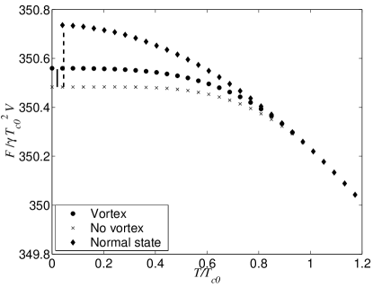
Figure 1: Plot of the free energy per unit volume of $N_{\sigma}=28000$ fermions in the normal, and superfluid phase with and without a vortex as a function of temperature. The solid and dashed vertical lines represent analytic expressions for the vortex and condensation energies, respectively.

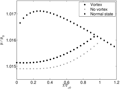
Figure 2: Chemical potential in the normal, and superfluid phase with and without a vortex, as determined by the constraint that $N_{\sigma}=28000$. We attribute the low temperature behavior of the normal phase chemical potential to shell effects due to the finite volume Schneider and Wallis (1998). For the vortex state the transition temperature is shifted downwards.

As can be seen from Fig. 2, the critical temperature for the vortex phase $T_{cv}$ is lower than that of the bulk superfluid phase without a vortex $T_{c0}$. For the specific parameters used, the difference is $1-T_{cv}/T_{c0}\approx 0.1$. This difference can be understood as follows: The vortex phase becomes unstable with respect to the normal phase when the extent of the vortex core becomes comparable to the radius $R$ of the system. Since the size of the vortex is ${\mathcal{O}}(\xi_{\rm BCS})$, we can estimate $T_{cv}$ from the condition $\xi_{\rm BCS}(T_{cv})\sim{\mathcal{O}}(R)$. Using $\Delta_{0}(T)\approx 1.7\Delta_{0}(0)(1-T/T_{c0})^{1/2}$ de Gennes (1989) for $0<1-T/T_{c0}\ll 1$, this yields

$$\frac{\delta T_{c}}{T_{c0}}\equiv 1-\frac{T_{cv}}{T_{c0}}\sim\frac{\xi_{\rm BCS}(0)^{2}}{R^{2}}\alpha_{1}$$ (34)

where $\alpha_{1}$ is a number of order one. We now test this expression and determine the constant $\alpha_{1}$ by numerically calculating the shift in the critical temperature $\delta T_{c}/{T_{c0}}$ due to the presence of a vortex for various radii of the system. The result is shown in Fig. 3. We find that we get reasonable agreement with Eq. (34) as $\xi_{\rm{BCS}}/R\rightarrow 0$ with a coefficient $\alpha_{1}\approx 2.3$. So one can understand decrease in $T_{c}$ due to the presence of the vortex as a finite size effect which scales as $\xi_{\rm BCS}(0)^{2}/R^{2}$.

Figure 3: The shift in the superfluid transition temperature for the vortex state relative to a bulk superfluid with no vortex, as a function of the radius of the confining cylinder at fixed density.

In Fig. 4 we plot the temperature dependence of the heat capacity $c_{\rm V}=(T/V)\partial S/\partial T$ per unit volume of the system. Again, we show for comparison results both for the system in the normal phase, in the superfluid phase without a vortex, and in the vortex phase. For a two component gas in the normal phase, we have $c_{\rm V\,normal}=\gamma T$ for $T\rightarrow 0$. The heat capacity for the superfluid phase without the vortex is exponentially damped by a factor $\exp(-\beta\Delta_{0})$ for $T\ll T_{c}$ due to the gap in the energy spectrum Fetter and Walecka (1971). Figure 4 on the other hand shows that the heat capacity in the vortex phase $c_{\rm V\,vortex}$ depends linearly on $T$ for low temperatures. This linear $T$-dependence is due to the presence of so-called core bound states in the vortex phase. These are single-particle excitations which are spatially localized in the vortex core where the gap is small. The energy of the core states is in general less than the bulk gap energy $\Delta_{0}$ and they exist only for angular momentum quantum numbers $m\geq 0$ de Gennes (1989). This corresponds to a quasi-particle current around the vortex core in the opposite direction to that of the vortex current. In a detailed analysis it was found that the energy spectrum of the lowest bound core states with $0\leq m\ll k_{F}\xi_{\rm BCS}$ for $T=0$ is essentially gapless and given by

$$E_{mk_{z}}\sim(m+1/2)\frac{\Delta_{0}^{2}}{\epsilon_{F}}\frac{h(\theta)}{\sin\theta}$$ (35)

where $k_{z}=k_{F}\cos\theta$ and $h(\theta)$ is a function of order unity Caroli et al. (1964). In Fig. 5, we plot the lowest quasi-particle energies as a function of $m$ for $k_{z}=0$ obtained from a numerical solution of Eq. (18). The gapless branch associated with the core states with energies less than $\Delta_{0}$ is clearly visible. The $T=0$ density of vortex states per unit volume is calculated by integrating Eq. (35) over $k_{z}$ which yields

$$N_{v}(\epsilon)=N(0)\alpha_{2}\frac{\xi_{\rm BCS}^{2}}{R^{2}}$$ (36)

for $0\ll\epsilon\ll\Delta_{0}$ where $\alpha_{2}\sim{\mathcal{O}}(1)$ Fetter1969 . Thus, the density of bound core states per unit volume is the same, apart from a factor $\alpha_{2}$, as that of a cylindrical region of a single component gas in the normal phase with radius $\xi_{\rm BCS}$ and length $L$. From this we conclude that the low $T$ heat capacity per unit volume of the gas in vortex phase $c_{\rm V\,vortex}$ associated with the core states is

$$c_{\rm V\,vortex}\sim c_{\rm V\,normal}\alpha_{2}\frac{\xi_{\rm BCS}^{2}}{R^{2}}$$ (37)

explaining the linear $T$-dependence of $c_{\rm V\,vortex}$ observed in Fig. 4. A fit to the numerical data yields $\alpha_{2}\approx 2$. We remark that a linear contribution to the heat capacity has been observed for a superconductor in the mixed state Keesom and Radebaugh (1964).

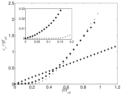
Figure 4: Plot of the specific heat per unit volume in the normal, and superfluid phase with and without a vortex. The inset shows the low temperature behavior for the vortex state and the superfluid state without a vortex (same symbols as in Figs. 1 and 2).

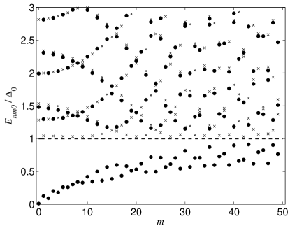
Figure 5: Energy spectrum for the lowest quasi-particle states in a superfluid with a vortex ($\bullet$) and the vortex free state ($\times$) at $T=0$. For clarity only the energies of states with $k_{z}=0$ have been plotted. There are branches of bound states for several values of $k_{z}$.

V Laser probing of the vortex phase

Vortices are now routinely created in dilute BECs where they can be detected by direct imaging of the cores, in which the density is significantly suppressed. Unfortunately, such a procedure would be very difficult to implement successfully for a dilute superfluid Fermi gas, where there is no significant depletion of density in the vortex core Nygaard et al. (2003). One way to observe the vortex is to measure the shift in the quadrupole mode frequencies which is directly proportional to the angular momentum per particle $\hbar/2$ associated with the supercurrent around the vortex core Bruun and Viverit (2001).

In the present section, we investigate the feasibility of detecting the bound quasi-particle states in the vortex core through a recently proposed laser probing scheme Törma and Zoller (2000); Bruun et al. (2001). The laser probing scheme is similar to scanning tunneling microscopy (STM) on a superconductor in that it relies on induced tunneling between a superfluid and a normal phase Hess et al. (1989, 1990). Whereas a STM probe uses a bias voltage to transfer population across a superconducting-normal interface existing between the normal microscope tip and the superconducting substrate, the laser probe instead creates an effective interface by coupling different internal states of the atoms by laser fields. Specifically, a spin state $|\uparrow\rangle$, which is Cooper paired with the state $|\downarrow\rangle$ is coupled via laser field to a third state $|e\rangle$ that has been chosen such that it does not participate in the pairing (either it does not have strong attractive interactions with the two other states or the disparity in chemical potentials is too large). Hence, the $|e\rangle$ atoms define the normal part of the interface. If the detuning of the laser from the atomic transition is $\delta=\omega_{A}-\omega_{L}$, where $\omega_{L}$ is the laser frequency and $\omega_{A}$ the frequency splitting between the level $|\uparrow\rangle$ and $|e\rangle$, the rate of change in the population of the $|e\rangle$ state (tunneling current) $I=-\langle\dot{\hat{N}_{e}}\rangle$ is Bruun et al. (2001)

$$I(\delta)= - \frac{2\pi}{\hbar}\sum_{\eta,n}\left|\int d^{3}r\,\Omega({\mathbf{r}})u_{\eta}({\mathbf{r}})\Phi^{*}_{n}({\mathbf{r}})\right|^{2}$$ (38)

$$\times [f(E_{\eta})-f(E_{n})]\delta(E_{\eta}-\epsilon_{n}-\tilde{\delta})$$

$$+ \left|\int d^{3}r\,\Omega({\mathbf{r}})v^{*}_{\eta}({\mathbf{r}})\Phi^{*}_{n}({\mathbf{r}})\right|^{2}[1-f(E_{\eta})-f(\xi_{n})]$$

$$\times \delta(E_{\eta}+\xi_{n}+\tilde{\delta}).$$

Here $\tilde{\delta}=\mu_{e}-\mu+\delta\equiv\Delta\mu+\delta$ is the effective detuning, $\mu_{e}$ the chemical potential of the $|e\rangle$ atoms, and $\Phi_{n}$ their single particle wave functions with energy $\xi_{n}$; $f(x)=[\exp(\beta x)+1]^{-1}$ is the Fermi function and $\Omega({\mathbf{r}})$ the Rabi frequency. In the present analysis, we assume for simplicity that the $|e\rangle$ atoms are non-interacting such that their wavefunctions $\Phi_{n}$ are the eigenstates of the confining cylindrical box. We consider the case of a constant laser profile $\Omega({\mathbf{r}})=\Omega$. This gives the selection rule ${\mathbf{k}}_{\uparrow}={\mathbf{k}}_{e}$ where ${\mathbf{k}}_{\uparrow}$ is the momentum of an $|\uparrow\rangle$ atom coupled by the laser beam to an $|e\rangle$ atom with momentum ${\mathbf{k}}_{e}$.

Let us now consider how the laser probing method can be used to probe the presence of the core states. We examine two opposite cases of interest: The case when there are initially no $|e\rangle$ atoms present ($N_{e}=0$) and the case where there initially are an equal number of $|\uparrow\rangle$ and $|e\rangle$ atoms present ($N_{\uparrow}=N_{e}$).

From Eq. (38) it is straightforward to show that for the total current we have $\int d\delta I(\delta)\propto N_{e}-N_{\uparrow}$. That is, the net current from the $|e\rangle$ atoms to the $|\uparrow\rangle$ atoms is proportional to the difference of initial populations between the two hyperfine states. Likewise, the total current from the core states trapped inside the vortex is clearly proportional to the total number of core states $N_{\rm cs}$. Thus, when there initially are no $|e\rangle$ atoms present ($N_{e}=0$) the spectral weight of the current due the core states as compared to the total current observed scales as $N_{\rm cs}/N_{\uparrow}$. Using $N_{\rm cs}\sim N_{v}\Delta_{0}\pi R^{2}L$ with $N_{v}$ given by Eq. (36), one obtains that the current from the core states divided by the total current scales as $\Delta_{0}\epsilon_{F}^{-1}\xi_{\rm BCS}^{2}R^{-2}\ll 1$. Thus, the signal from the core states is completely overwhelmed by the bulk signal coming from the current out of the whole Fermi sea of $|\uparrow\rangle$ atoms. We therefore conclude that it is most likely not possible to probe the core states starting with initially no $|e\rangle$ present. This conclusion is supported by numerical simulations.

Let us therefore consider the case when there initially are an equal number of $|\uparrow\rangle$ and $|e\rangle$ atoms present ($N_{\uparrow}=N_{e}$). In that way, the bulk signal of transitions of $|\uparrow\rangle$ atoms deep within the Fermi sea is Pauli blocked due to the presence of the $|e\rangle$ atoms since we have the selection rule ${\mathbf{k}}_{\uparrow}={\mathbf{k}}_{e}$. One can then show from Eq. (38) that the total signal scales as $\int d\delta|I(\delta)|\propto N_{\uparrow}\Delta_{0}/\epsilon_{F}$, i.e. the current is proportional to the total number of Cooper pairs. Thus, the bulk signal is suppressed by a factor $\Delta_{0}/\epsilon_{F}$ compared to the case when there are no $|e\rangle$ atoms present simply due to the Fermi blocking effect. The current due to the vortex core states should therefore be easier to observe as it is not overwhelmed by a huge background signal. In Fig. 6 we plot the $T=0$ laser probing current $I(\delta)$ for the case when $N_{e}=N_{\uparrow}$. The effect of the Hartree field $gn_{\sigma}$ is primarily to shift the entire profile to lower detunings $\delta$ since it shifts the energies of the $|\uparrow\rangle$ atoms by the amount $gn_{\sigma}$ whereas the $|e\rangle$ atoms are assumed non-interacting. In the plot we have explicitly eliminated this overall shift for reasons of clarity. We plot the current both when there is no vortex present and when there is a vortex. In the case of no vortex present, the current given by Eq. (38) at zero temperature can be shown to be

$$I=\pm\pi\Omega^{2}\rho(\delta)\,\Theta(\delta^{2}-\Delta_{0}^{2})\frac{\Delta_{0}^{2}}{\delta^{2}},$$ (39)

where $\pm$ corresponds to $\delta>0$ and $\delta<0$ respectively and $\rho(\delta)=V(\Delta_{0}^{2}/\delta-\delta+2\mu)^{1/2}/2\pi^{2}$ Törma and Zoller (2000); Bruun et al. (2001). From Eq. (39) it follows that there is no current for detunings with $-\Delta_{0}<\delta<\Delta_{0}$. This can be interpreted as the laser signal has to provide a minimum energy $\Delta_{0}$ to break a Cooper pair and generate a current. Equation (39) is also shown on Fig. 6 and we see good agreement with the numerical result when there is no vortex present. Note that since the numerical calculations use a Lorentzian of width $\Gamma=0.01\Delta_{0}$ instead of $\delta(x)$ functions in Eq. (38), we have convoluted Eq. (39) accordingly. We see that the signal when there is a vortex present is markedly different from the case with no vortex. In particular, there is a significant current for $|\delta|<\Delta_{0}$. This current is directly due to the presence of the core states which have a pairing energy less than $\Delta_{0}$. The signal from the vortex phase is finite for $\delta\sim 0$ reflecting the fact that the energy spectrum of the core states approximately given by Eq. (35) is essentially gapless. Thus, the existence of core states bound in the vortex is reflected in the current profile $I(\delta)$.

Figure 6: The tunneling current as a function of detuning (in units of the bulk value of the gap) for tunneling into filled state from both a vortex state and a superfluid without a vortex. For comparison Eq. (39) is also plotted. The profiles have been shifted to compensate for the Hartree mean field shift $gn_{\sigma}$ of the energies of the $|\uparrow\rangle$ atoms. If the $|\uparrow\rangle$ atoms are in the normal state no current flows due to Pauli blocking.

VI Conclusions

We have studied the properties of a single vortex in a neutral superfluid with Fermi statistics using a microscopic weak coupling theory. The effect of the vortex on the free energy and the heat capacity of the system was examined and we provided various analytical expressions which agrees well with the numerical results. The vortex gives rise to the presence of core states bound in the vortex core. We examined the spectrum of these states and also suggested a way to experimentally detect them. Apart from being of interest theoretically, it is not unlikely that our results will have experimental relevance in the near future due to the recent impressive experimental progress within the field of atomic Fermi gases.

References

- DeMarco and Jin (1999) B. DeMarco and D. S. Jin, Science 285, 1703 (1999).
- Truscott et al. (2001) A. W. Truscott, K. E. Strecker, W. I. McAlexander, G. B. Partridge, and R. G. Hulet, Science 291, 2570 (2001).
- Schreck et al. (2001) F. Schreck, G. Ferrari, K. L. Corwin, J. Cubizolles, L. Khaykovich, M. O. Mewes, and C. Salomon, Phys. Rev. A 64, 011402(R) (2001).
- Granade et al. (2002) S. R. Granade, M. E. Gehm, K. M. O’Hara, and J. E. Thomas, Phys. Rev. Lett. 88, 120405 (2002).
- Hadzibabic et al. (2002) Z. Hadzibabic, C. A. Stan, K. Dieckmann, S. Gupta, M. W. Zwierlein, A. Görlitz, and W. Ketterle, Phys. Rev. Lett. 88, 160401 (2002).
- Roati et al. (2002) G. Roati, F. Riboli, G. Modugno, and M. Inguscio, Phys. Rev. Lett. 89, 150403 (2002).
- Jochim et al. (2002) S. Jochim, M. Bartenstein, G. Hendl, J. H. Denschlag, R. Grimm, A. Mosk, and M. Weidemüller, Phys. Rev. Lett. 89, 273202 (2002).
- Feshbach (1958) H. Feshbach, Ann. Phys. 5, 357 (1958).
- Feshbach (1962) H. Feshbach, Ann. Phys. 19, 287 (1962).
- Tiesinga et al. (1993) E. Tiesinga, B. J. Verhaar, and H. T. C. Stoof, Phys. Rev. A 47, 4114 (1993).
- Stoof et al. (1996) H. T. C. Stoof, M. Houbiers, C. A. Sackett, and R. G. Hulet, Phys. Rev. Lett. 76, 10 (1996).
- Matthews et al. (1999) M. R. Matthews, B. P. Anderson, P. C. Haljan, D. S. Hall, C. E. Wieman, and E. A. Cornell, Phys. Rev. Lett. 83, 2498 (1999).
- Madison et al. (2000) K. W. Madison, F. Chevy, W. Wohlleben, and J. Dalibard, Phys. Rev. Lett. 84, 806 (2000).
- Baranov and Petrov (2000) M. A. Baranov and D. S. Petrov, Phys. Rev. A 62, 041601 (2000).
- Bruun and Mottelson (2001) G. M. Bruun and B. R. Mottelson, Phys. Rev. Lett. 87, 270403 (2001).
- Nygaard et al. (2003) N. Nygaard, G. M. Bruun, C. W. Clark, and D. L. Feder, Phys. Rev. Lett. 90, 210402 (2003).
- Bruun and Viverit (2001) G. M. Bruun and L. Viverit, Phys. Rev. A 64, 063606 (2001).
- Holland et al. (2001) M. Holland, S. J. J. M. F. Kokkelmans, M. L. Chiofalo, and R. Walser, Phys. Rev. Lett. 87, 120406 (2001).
- Timmermans et al. (2001) E. Timmermans, K. Furuya, P. W. Milonni, and A. K. Kerman, Phys. Lett. A 285, 228 (2001).
- O’Hara et al. (2002) K. M. O’Hara, S. L. Hemmer, M. E. Gehm, S. R. Granade, , and J. E. Thomas, Scince 298, 2179 (2002).
- Bourdel et al. (2003) T. Bourdel, J. Cubizolles, L. Khaykovich, K. M. F. Magalhes, S. J. J. M. F. Kokkelmans, G. V. Shlyapnikov, and C. Salomon, Phys. Rev. Lett. 91, 020402 (2003).
- Strecker et al. (2003) K. E. Strecker, G. B. Partridge, and R. G. Hulet, Phys. Rev. Lett. 91, 080406 (2003).
- Greiner et al. (doi:10.1038/nature02199) M. Greiner, C. A. Regal, and D. S. Jin, Nature advance online publication, 26 November 2003 (doi:10.1038/nature02199).
- Jochim et al. (10.1126/science.1093280) S. Jochim, M. Bartenstein, A. Altmeyer, G. Hendl, S. Riedl, C. Chin, J. D. Denschlag, and R. Grimm, Science, November 13 2003 (10.1126/science.1093280).
- Zwierlein et al. (2003) M. W. Zwierlein, C. A. Stan, C. H. Schunck, S. M. F. Raupach, S. Gupta, Z. Hadzibabic, and W. Ketterle, cond-mat/0311617 (2003).
- Hofstetter et al. (2002) W. Hofstetter, J. I. Cirac, P. Zoller, E. Demler, and M. D. Lukin, Phys. Rev. Lett. 89, 220407 (2002).
- Anderson and Kasevich (1998) B. P. Anderson and M. A. Kasevich, Science 282, 1686 (1998).
- Orzel et al. (2001) C. Orzel, A. K. Tuchman, M. L. Fenselau, M. Yasuda, and M. A. Kasevich, Scince 291, 2386 (2001).
- Greiner et al. (2002) M. Greiner, O. Mandel, T. Esslinger, T. W. Hänsch, and I. Bloch, Nature (London) 415, 39 (2002).
- de Gennes (1989) P. G. de Gennes, Superconductivity of metals and alloys (Addison-Wesley, New York, 1989).
- Bruun et al. (1999) G. Bruun, Y. Castin, R. Dum, and K. Burnett, Euro. Phys. J. D 7, 433 (1999).
- Bulgac and Yu (2002) A. Bulgac and Y. Yu, Phys. Rev. Lett. 88, 042504 (2002).
- Grasso and Urban (2003) M. Grasso and M. Urban, Phys. Rev. A 68, 033610 (2003).
- (34) We can estimate the radius of the cylinder in which interior superfluidity will be suppressed by equating the kinetic energy with the condensation energy per particle . This gives just .
- Baye and Heenen (1986) D. Baye and P.-H. Heenen, J. Phys. A: Math. Gen. 19, 2041 (1986).
- Light and Carrington (2000) J. C. Light and T. Carrington, Jr., Adv. Chem. Phys. 114, 263 (2000).
- Lemoine (1994) D. Lemoine, J. Chem. Phys. 101, 1 (1994).
- Arfken and Weber (1995) G. B. Arfken and H. J. Weber, Mathematical Methods for Physicists (Academic Press, San Diego, 1995), 4th ed.
- Fetter and Walecka (1971) A. L. Fetter and J. D. Walecka, Quantum theory of many-particle systems (McGraw-Hill, New York, 1971).
- Schneider and Wallis (1998) J. Schneider and H. Wallis, Phys. Rev. A 57, 1253 (1998).
- Caroli et al. (1964) C. Caroli, P. G. D. Gennes, and J. Matricon, Phys. Lett. 9, 307 (1964).
- (42) A. L. Fetter, in Superconductivity, edited by R. D. Parks (Marcel Dekker, Inc., New York, 1969), Vol. I.
- Keesom and Radebaugh (1964) P. H. Keesom and R. Radebaugh, Phys. Rev. Lett. 13, 685 (1964).
- Törma and Zoller (2000) P. Törma and P. Zoller, Phys. Rev. Lett. 85, 487 (2000).
- Bruun et al. (2001) G. M. Bruun, P. Törma, M. Rodriguez, and P. Zoller, Phys. Rev. A 64, 033609 (2001).
- Hess et al. (1989) H. F. Hess, R. B. Robinson, R. C. Dynes, J. M. Valles, Jr., and J. V. Waszczak, Phys. Rev. Lett. 62, 214 (1989).
- Hess et al. (1990) H. F. Hess, R. B. Robinson, and J. V. Waszczak, Phys. Rev. Lett. 64, 2711 (1990).