Steady shear flow thermodynamics based on a canonical distribution approach

Abstract

A non-equilibrium steady state thermodynamics to describe shear flows is developed using a canonical distribution approach. We construct a canonical distribution for shear flow based on the energy in the moving frame using the Lagrangian formalism of the classical mechanics. From this distribution we derive the Evans-Hanley shear flow thermodynamics, which is characterized by the first law of thermodynamics $d\mathcal{E}=Td\mathcal{S}-\mathcal{Q}d\gamma$ relating infinitesimal changes in energy $\mathcal{E}$, entropy $\mathcal{S}$ and shear rate $\gamma$ with kinetic temperature $T$. Our central result is that the coefficient $\mathcal{Q}$ is given by Helfand’s moment for viscosity. This approach leads to thermodynamic stability conditions for shear flow, one of which is equivalent to the positivity of the correlation function of $\mathcal{Q}$. We emphasize the role of the external work required to sustain the steady shear flow in this approach, and show theoretically that the ensemble average of its power $\dot{W}$ must be non-negative. A non-equilibrium entropy, increasing in time, is introduced, so that the amount of heat based on this entropy is equal to the average of $\dot{W}$. Numerical results from non-equilibrium molecular dynamics simulation of two-dimensional many-particle systems with soft-core interactions are presented which support our interpretation.

Pacs numbers: 05.70.Ln, 83.50.Ax, 05.20.Jj, 83.60.Rs

I Introduction

The great success of thermodynamics as a physical theory to describe various equilibrium phenomena has stimulated attempts to generalize it to a theory applicable to macroscopic time-dependent phenomena, namely to a non-equilibrium thermodynamics. Many efforts have been devoted to this subject, and led to some proposals for non-equilibrium thermodynamics, for example, the classical irreversible thermodynamics Gro84 , the rational thermodynamics Tru84 ; Lav93 and the extended irreversible thermodynamics Jou01 . Recently, a non-equilibrium thermodynamics, which tries to give more rigorous predictions by restricting its applied field into non-equilibrium steady states, is also discussed Ono98 ; Hat01 ; Sas01 .

Shear flow is a typical example of non-equilibrium steady phenomena. For a constant velocity gradient it has a steady current (the shear stress), and has many applications in the investigation of rheological properties of materials Bar89 ; Tsh89 . Such models have been widely used to calculate the shear viscosity, whose shear rate dependence is still actively discussed Tra95 ; Mat00 ; Mar01a ; Ge01 . The apparent existence of critical phenomenon, appearing as a transition from a uniform bulk phase to an organized string-like phase, is shown at high shear rate Erp84 ; Woo84 ; Hey85 . It is used as an application of non-Hamiltonian molecular dynamics called the non-equilibrium thermostated dynamics Eva90a , by which some non-equilibrium dynamical properties such as the conjugate pairing rule for the Lyapunov spectrum Dre88 ; Eva90b ; Det96a ; Tan02 and the fluctuation theorem Eva93 ; Gal95 were discussed. Shear flow has also been described by the Bhatnagar-Gross-Krook kinetic equation, which is a simplification of the Boltzmann equation, and using this equation, transport coefficients and hydrodynamic modes were calculated Zwa79 ; San91 ; Lee97 . Steady shear flow is a spatially homogenous and time-independent phenomenon, so a simple description compared to general non-equilibrium phenomena may be expected. However, although it is such a simple steady non-equilibrium phenomenon, a convincing thermodynamic description of shear flow is not known yet.

A proposed non-equilibrium steady state thermodynamics to describe shear flow was given by Evans and Hanley Eva80a ; Eva80b ; Han82 ; Eva83 . It expresses the first law of thermodynamics for the shear flow by adding the term $\xi d\gamma$ expressing the response to a shear rate $\gamma$, namely

$$d\mathcal{E}=Td\mathcal{S}+\xi d\gamma$$ (1)

as a relation among infinitesimal quasi-static changes of internal energy $\mathcal{E}$, entropy $\mathcal{S}$ and the shear rate $\gamma$ with temperature $T$ and the coefficient $\xi$ defined by $\xi\equiv\partial\mathcal{E}/\partial\gamma|_{\mathcal{S}}$ noteI1 . As a conceptual feature, the Evans-Hanley thermodynamics is characterized by the fact that the shear rate is an external parameter chosen as an additional variable to describe non-equilibrium effects. This is analogous to the choice of variables in equilibrium thermodynamics where the variables are chosen as parameters manipulated externally, for example, the temperature and volume, etc. This choice of thermodynamic variables has the advantage that observables in this approach are rather easy to access by experiments and computer simulations. This feature also distinguishes the Evans-Hanley thermodynamics from some other non-equilibrium thermodynamics, in which local quantities related to conserved quantities, such as the local momentum density, are chosen as additional variables to describe non-equilibrium effects, because they change slowly with time and are consistent with the phenomenological equations of hydrodynamics. Compared with such a general formalism of non-equilibrium thermodynamics, the Evans-Hanley thermodynamics gives a much simpler description, as its applied field is restricted to steady shear flow. On the other hand, one of the problems in the Evans-Hanley shear flow thermodynamics was that a clear physical meaning for the coefficient $\xi$, especially its microscopic expression, was not known, so that one has not had clear experimental or numerical evidence to support this thermodynamics. On this point, Ref. Eva89 tried to calculate numerically a value of $\xi$ by introducing a non-equilibrium entropy in a low density system. Also recently, Ref. Dai03 discussed a phenomenological expression for $\xi$ using the Maxwell model for shear flow.

Another important aspect of non-equilibrium thermodynamics is its construction from a solid statistical mechanical foundation. Some attempts in this direction have been discussed using the non-equilibrium canonical distribution approach Mor56 ; Kub57 ; Mor58 ; Yam67 ; Kaw73 ; Zub74 and the projection operator approach Zwa61 ; Mor65 ; Rob65 ; Rob67 ; Gro82 ; Tan97 and so on. As one such approach, the non-equilibrium canonical distribution approach justifies the response formula for thermodynamic perturbations, which is different from a mechanical perturbation expressed as a change in an external parameter appearing explicitly in the Hamiltonian Kub78 . It uses, in principle, the distribution $f(\mbox{\boldmath$\bf\Gamma$})$ of canonical type

$$f(\mbox{\boldmath$\bf\Gamma$})=\Xi^{-1}\exp\left\{-\beta\left[H(\mbox{\boldmath$\bf\Gamma$})+\sum_{\alpha=1}^{\tilde{n}}\mu_{\alpha}(\mbox{\boldmath$\bf\Gamma$})A_{\alpha}(\mbox{\boldmath$\bf\Gamma$})\right]\right\}$$ (2)

where $\Xi$ is a normalization constant, $\beta$ is the inverse temperature, $H(\mbox{\boldmath$\bf\Gamma$})$ is the Hamiltonian as a function of the phase space vector $\bf\Gamma$, and $\mu_{\alpha}(\mbox{\boldmath$\bf\Gamma$})$ and $A_{\alpha}(\mbox{\boldmath$\bf\Gamma$})$ are pairs of conjugate variables whose forms depend on the non-equilibrium phenomena under consideration. In many cases, the distribution $f(\mbox{\boldmath$\bf\Gamma$})$, and therefore the functions $\mu_{\alpha}(\mbox{\boldmath$\bf\Gamma$})$ and $A_{\alpha}(\mbox{\boldmath$\bf\Gamma$})$, $\alpha=1,2,\cdots,\tilde{n}$, is introduced based on the ”local equilibrium assumption” Zub74 , although it is not always necessary. Using the distribution $f(\mbox{\boldmath$\bf\Gamma$})$ and the Liouville operator $\hat{L}$, we calculate average quantities as the ensemble average under time-evolution of the distribution function

$$\tilde{f}(\mbox{\boldmath$\bf\Gamma$},t) \equiv \exp\left\{-i\hat{L}(t-t_{0})\right\}f(\mbox{\boldmath$\bf\Gamma$}),$$ (3)

which may be regarded as the distribution function at time $t$ evolved from the initial canonical distribution function $f(\mbox{\boldmath$\bf\Gamma$})$ at time $t_{0}$. In this way, we can derive the thermal response formula for viscosity, thermal conductivity and so on Mor58 ; Yam67 ; Kaw73 ; Zub74 . This approach was generalized to non-Hamiltonian systems such as the Sllod equation for shear flow systems with isokinetic thermostat Mor85 ; Mor88 ; Sar98 , and was used to calculate some thermal quantities, such as the specific heat of non-equilibrium steady states Eva87a ; Eva87b . However it is still an open problem to construct the Evans-Hanley shear flow thermodynamics from this non-equilibrium canonical distribution approach based on distributions of this type (2). Usually, the thermodynamic relation for the first law of thermodynamics in the canonical distribution approach is introduced based upon the local equilibrium assumption, but the form (1) as the first law of thermodynamics for shear flow cannot be justified by this assumption, because Eq. (1) including the term $\xi d\gamma$ expressing the non-equilibrium effect of the shear flow cannot be attributed to an equilibrium thermodynamical relation even if we consider a very small portion of system.

The principal aim of this paper is to derive the Evans-Hanley shear flow thermodynamics based on the canonical distribution approach to non-equilibrium steady states. First we show that the canonical distribution for shear flow is represented by the distribution (2) in the case where $\tilde{n}=1$, $\mu_{\alpha}(\mbox{\boldmath$\bf\Gamma$})=\gamma$ and $A_{\alpha}(\mbox{\boldmath$\bf\Gamma$})=-Q(\mbox{\boldmath$\bf\Gamma$})$. Here $Q(\mbox{\boldmath$\bf\Gamma$})$ is the Helfand moment of viscosity and its time-derivative is connected with the off-diagonal component of the pressure tensor. The canonical distribution given here is different from the canonical distribution based on the local equilibrium assumption, because the ”non-equilibrium term” $-\gamma Q(\mbox{\boldmath$\bf\Gamma$})$ in the distribution $f(\mbox{\boldmath$\bf\Gamma$})$ cannot be neglected even if we take the system size to be very small. So to derive the canonical distribution for shear flow, we introduce the Hamiltonian for the moving frame which follows the steady global current, then using the Lagrangian techniques of classical mechanics, and the fact that the quantity $H(\mbox{\boldmath$\bf\Gamma$})+\sum_{\alpha=1}^{\tilde{n}}\mu_{\alpha}(\mbox{\boldmath$\bf\Gamma$})A_{\alpha}(\mbox{\boldmath$\bf\Gamma$})$ in the distribution (2) should correspond to this moving frame Hamiltonian. This procedure, which is one of the important points of this paper, gives a systematic way to choose the function $\sum_{\alpha=1}^{\tilde{n}}\mu_{\alpha}(\mbox{\boldmath$\bf\Gamma$})A_{\alpha}(\mbox{\boldmath$\bf\Gamma$})$ for the canonical distribution approach to non-equilibrium steady states. To justify this procedure concretely, we show that by applying it to the rotating system we can obtain the well known canonical distribution for the rotating system, and therefore its thermodynamics.

Second we show that our approach is consistent with the linear response formula for viscosity, which can be derived from the ensemble average of the shear stress using the distribution (3). To interpret the derivation of this response formula we emphasize the role of the work required to sustain the steady shear flow. We introduce a non-equilibrium entropy, which increases in time, and show that the heat based on this entropy has the same magnitude as the power needed to sustain the shear flow.

Third we derive the form (1) of the first law of thermodynamics for shear flow from our canonical distribution approach, and show that the quantity $\xi$ in the form (1) is given by $\xi=-\overline{Q}$ with $\overline{Q}$ being the ensemble average of the Helfand moment for viscosity $Q(\mbox{\boldmath$\bf\Gamma$})$. We also discuss the thermodynamic stability condition for shear flow, which leads to the positivity of the correlation function of $Q(\mbox{\boldmath$\bf\Gamma$})$ as well as the positivity of the specific heat.

Finally we present some numerical calculations of many-particle systems with soft-core interactions to support our thermodynamic interpretation of steady shear flow. Here, we use the Sllod equations with the isokinetic thermostat and Lee-Edwards boundary condition Lee72 . In these simulations we show the shear rate dependences of the average of Helfand’s moment of viscosity, its correlation function and the work needed to sustain the shear flow.

II Canonical Distribution for Steady Flows

II.1 Moving Frame and Energy

Systems discussed in this paper are steady flows, in which the global velocity distribution of the flow is given by a time-independent function $\mathbf{V}(\textbf{r})$ at the position r in the inertial frame $\mathcal{F}^{(ine)}$. We consider a system which consists of $N$ particles with the same mass $m$ and is described by classical mechanics (without magnetic fields).

In this section we use the Lagrangian formalism of classical mechanics to compare quantities in different frames. The Lagrangian formalism is a direct consequence of the frame-independent principle of least action $\delta\int_{t_{1}}^{t_{2}}dtL=0$ for fixed values of positions at times $t_{1}$ and $t_{2}$, where $L$ is the Lagrangian as a function of particle positions and velocities.

In the inertial frame $\mathcal{F}^{(ine)}$ the Lagrangian $L^{(ine)}=L^{(ine)}(\mathbf{v}^{(ine)},\mathbf{q})$ is given by

$$L^{(ine)}(\mathbf{v}^{(ine)},\mathbf{q})=\frac{1}{2}m\left|{\mathbf{v}^{(ine)}}\right|^{2}-U(\mathbf{q})$$ (4)

as a function of $\mathbf{v}^{(ine)}\equiv(\mathbf{v}_{1}^{(ine)},\mathbf{v}_{2}^{(ine)},\cdots,\mathbf{v}_{N}^{(ine)})$ and $\mathbf{q}\equiv(\mathbf{q}_{1},\mathbf{q}_{2},\cdots,\mathbf{q}_{N})$, where $\mathbf{v}_{j}^{(ine)}$ and $\mathbf{q}_{j}$ are the velocity and the spatial position of the $j$-th particle, respectively, and $U(\mathbf{q})$ is the potential function as a function of $\mathbf{q}$. Using the definitions $\mathbf{p}^{(ine)}\equiv\partial L^{(ine)}/\partial\mathbf{v}^{(ine)}$ and $H^{(ine)}(\mathbf{p}^{(ine)},\mathbf{q})\equiv\mathbf{p}^{(ine)}\cdot\mathbf{v}^{(ine)}-L^{(ine)}$, the Lagrangian (4) leads to expressions for the momentum $\mathbf{p}^{(ine)}$ and the Hamiltonian $H^{(ine)}$ as

$$\mathbf{p}^{(ine)}=m\mathbf{v}_{j}^{(ine)}$$ (5)

$$H^{(ine)}(\mathbf{p}^{(ine)},\mathbf{q})=\frac{1}{2m}\left|\mathbf{p}^{(ine)}\right|^{2}+U(\mathbf{q}).$$ (6)

Here we note that the Hamiltonian $H^{(ine)}$ is a function of $\mathbf{p}^{(ine)}$ and $\mathbf{q}$, namely $H^{(ine)}=H^{(ine)}(\mathbf{p}^{(ine)},\mathbf{q})$.

Now, we introduce the velocity $\mathbf{v}_{j}^{(mov)}$ of the $j$-th particle in the moving frame $\mathcal{F}^{(mov)}$, which is connected to the velocity $\mathbf{v}_{j}^{(ine)}$ in the inertial frame $\mathcal{F}^{(ine)}$ by

$$\mathbf{v}_{j}^{(mov)}\equiv\mathbf{v}_{j}^{(ine)}-\mathbf{V}(\textbf{q}_{j}).$$ (7)

The quantity $\mathbf{v}_{j}^{(mov)}$ is often referred to as the thermal velocity of particle $j$. The position q is invariant under this frame change $\mathcal{F}^{(ine)}\rightarrow\mathcal{F}^{(mov)}$. Inserting the velocity $\mathbf{v}_{j}^{(ine)}=\mathbf{v}_{j}^{(mov)}+\mathbf{V}(\textbf{q}_{j})$ into Eq. (4), the Lagrangian $L^{(mov)}=L^{(mov)}(\mathbf{v}^{(mov)},\mathbf{q})$ of the system in the moving frame $\mathcal{F}^{(mov)}$ is given by

$$L^{(mov)}(\mathbf{v}^{(mov)},\mathbf{q})=L^{(ine)}$$

$$=\frac{1}{2}m\sum_{j=1}^{N}\left|{\mathbf{v}_{j}^{(mov)}}+\mathbf{V}(\textbf{q}_{j})\right|^{2}-U(\mathbf{q})$$ (8)

as a function of $\mathbf{v}^{(mov)}\equiv(\mathbf{v}_{1}^{(mov)},\mathbf{v}_{2}^{(mov)}\cdots,\mathbf{v}_{N}^{(mov)})$ and $\mathbf{q}$. Equation (8) leads to the momentum $\mathbf{p}^{(mov)}\equiv\partial L^{(mov)}/\partial\mathbf{v}^{(mov)}$ as

$$\mathbf{p}_{j}^{(mov)} = m\left[\mathbf{v}_{j}^{(mov)}+\mathbf{V}(\textbf{q}_{j})\right]$$ (9)

$$= m\mathbf{v}_{j}^{(ine)}=\mathbf{p}_{j}^{(ine)}.$$

Therefore the momentum is independent of choice of the frames $\mathcal{F}^{(mov)}$ and $\mathcal{F}^{(ine)}$, and hereafter we use the notation $\mathbf{p}\equiv(\mathbf{p}_{1},\mathbf{p}_{2}\cdots,\mathbf{p}_{N})\equiv\mathbf{p}^{(mov)}=\mathbf{p}^{(ine)}$ for the momentum, and also use the notation $\mbox{\boldmath$\bf\Gamma$}\equiv(\mathbf{p},\mathbf{q})$ for the phase space vector. On the other hand, the Hamiltonian $H^{(mov)}=H^{(mov)}(\mbox{\boldmath$\bf\Gamma$})$ in the moving frame $\mathcal{F}^{(mov)}$ is given by

$$H^{(mov)}(\mbox{\boldmath$\bf\Gamma$})=H^{(ine)}(\mbox{\boldmath$\bf\Gamma$})-\sum_{j=1}^{N}\mathbf{p}_{j}\cdot\mathbf{V}(\textbf{q}_{j}).$$ (10)

using the definition $H^{(mov)}(\mbox{\boldmath$\bf\Gamma$})\equiv\mathbf{p}\cdot\mathbf{v}^{(mov)}-L^{(mov)}$ and Eq. (6). It is essential to note that although the momenta $\mathbf{p}^{(mov)}$ and $\mathbf{p}^{(ine)}$ are equal, the Hamiltonian $H^{(mov)}(\mbox{\boldmath$\bf\Gamma$})$ in the moving frame $\mathcal{F}^{(mov)}$ is different from the Hamiltonian $H^{(ine)}(\mbox{\boldmath$\bf\Gamma$})$ in the inertial frame $\mathcal{F}^{(ine)}$ and their difference is proportional to the global current distribution $\mathbf{V}(\textbf{q}_{j})$ note2 .

II.2 Canonical Distribution

The central assumption of this paper is that in the moving frame $\mathcal{F}^{(mov)}$ defined by the global velocity distribution $\mathbf{V}(\textbf{r})$ the system can be regarded as an equilibrium state. It is important to note that this assumption is not obvious, because generally a global flow causes some local effects such as string phases in shear flows Erp84 ; Woo84 ; Hey85 ; Eva90a and possibly turbulent phases and so on, which can destroy this assumption. However these phases generally occur in far-from equilibrium states so we may expect that our assumption is satisfied in a regime near equilibrium. Under this assumption, we introduce the canonical distribution

$$f(\mbox{\boldmath$\bf\Gamma$}) = \Xi^{-1}\exp\left\{-\beta H^{(mov)}(\mbox{\boldmath$\bf\Gamma$})\right\}$$

$$= \Xi^{-1}\exp\left\{-\beta\left[H^{(ine)}(\mbox{\boldmath$\bf\Gamma$})-\sum_{j=1}^{N}\mathbf{p}_{j}\cdot\mathbf{V}(\textbf{q}_{j})\right]\right\}$$

for steady flow, where $\beta$ is the inverse temperature $1/(k_{B}T)$ with the Boltzmann constant $k_{B}$ and the temperature $T$, and $\Xi$ is the partition function $\Xi\equiv\int d\mbox{\boldmath$\bf\Gamma$}\exp\left\{-\beta H^{(mov)}(\mbox{\boldmath$\bf\Gamma$})\right\}$. For simplicity we use units so that $k_{B}=1$ hereafter in this paper. It should be noted that the function $f(\mbox{\boldmath$\bf\Gamma$})$ is the distribution of $\textbf{p}^{(ine)}$ and q in the inertial frame $\mathcal{F}^{(ine)}$, as well as the distribution of $\textbf{p}^{(mov)}$ and q in the moving frame $\mathcal{F}^{(mov)}$, because of the identity of the momenta implies $\mbox{\boldmath$\bf\Gamma$}=(\mathbf{p}^{(ine)},\mathbf{q})=(\mathbf{p}^{(mov)},\mathbf{q})$.

The canonical distribution (LABEL:Canon) is different from that obtained from the ”local equilibrium assumption”, which is popular in many texts on non-equilibrium statistical mechanics. In this approach the canonical distribution function $g(\mbox{\boldmath$\bf\Gamma$})$ is chosen as

$$g(\mbox{\boldmath$\bf\Gamma$})$$

$$\equiv\tilde{\Xi}^{-1}\exp\left\{-\beta\left[\sum_{j=1}^{N}\frac{1}{2m}\left|\mathbf{p}-m\mathbf{V}(\textbf{q}_{j})\right|^{2}+U(\mathbf{q})\right]\right\}$$

$$=\tilde{\Xi}^{-1}\exp\left\{-\beta\left[H^{(mov)}(\mbox{\boldmath$\bf\Gamma$})+\sum_{j=1}^{N}\frac{1}{2}m\left|\mathbf{V}(\textbf{q}_{j})\right|^{2}\right]\right\}$$

(13)

with $\tilde{\Xi}\equiv\int d\mbox{\boldmath$\bf\Gamma$}\exp\{-\beta[\sum_{j=1}^{N}|\mathbf{p}-m\mathbf{V}(\textbf{q}_{j})|^{2}/(2m)+U(\mathbf{q})]\}$. This type of distribution was actually used to calculate the shear viscosity Zwa79 ; San91 ; Mor56 ; Yam67 ; Kaw73 , and its localized version was used as a canonical distribution under the local equilibrium assumption (See for example, Ref. Zub74 ). However it is not consistent with the thermodynamics of rotating systems discussed in the next subsection, so the difference between the two distributions (LABEL:Canon) and (13) is crucial to the subject of this paper, that is a statistical foundation for steady state thermodynamics. Another problem with the distribution $g(\mbox{\boldmath$\bf\Gamma$})$ is that it does not take into account the inertial force. Despite these problems, one may also notice that the deviation of the distribution (13) from the distribution (LABEL:Canon) is of order $\mathcal{O}(|\mathbf{V}|^{2})$ in the global velocity, and near equilibrium it may give small effects compared with the effects given by the second term on the right-hand side of Eq. (10) which is of order $\mathcal{O}(|\mathbf{V}|)$.

III Rotating Systems and their Thermodynamics

Before discussing the canonical distribution approach to shear flow systems, in this section we give a derivation of the well known canonical distribution and the thermodynamics for uniformly rotating systems, based on the formalism given in Sec. II. The rotating system is a typical example to which our approach can be applied, and a comparison between the rotating system and the shear flow system gives a useful insight into the canonical distribution approach and the thermodynamics of shear flow systems which will be developed in Secs. IV and V.

III.1 Canonical Distribution for Rotating Systems

We consider a rotating system with a constant angular velocity vector $\bf\omega$. We assume that the Hamiltonian $H^{(ine)}(\mbox{\boldmath$\bf\Gamma$})$ is invariant under rotation about the axis of rotation. In this section the origin of the spatial coordinates and the axis of rotation is taken at the center of mass of the system. Under these conditions the global velocity distribution function $\mathbf{V}$ is given by

$$\mathbf{V}(\mathbf{q}_{j})=\mbox{\boldmath$\bf\omega$}\times\mathbf{q}_{j}$$ (14)

where $\times$ is the usual vector product. This global velocity distribution can be sustained without any external effect in isolated systems, because of the conservation of the total angular momentum.

Using Eq. (14), relation (10) is rewritten as

$$H^{(mov)}(\mbox{\boldmath$\bf\Gamma$})=H^{(ine)}(\mbox{\boldmath$\bf\Gamma$})-\mbox{\boldmath$\bf\omega$}\cdot\mathbf{M}(\mbox{\boldmath$\bf\Gamma$})$$ (15)

with the total angular momentum $\mathbf{M}(\mbox{\boldmath$\bf\Gamma$})\equiv\sum_{j=1}^{N}\textbf{q}_{j}\times\mathbf{p}_{j}.$ In comparison with shear flow systems discussed in Sec. IV, it is important to note that the total angular momentum $\mathbf{M}(\mbox{\boldmath$\bf\Gamma$})$ is conserved in the inertial frame $\mathcal{F}^{(ine)}$, namely

$$i\hat{L}^{(ine)}\mathbf{M}(\mbox{\boldmath$\bf\Gamma$})=0,$$ (16)

where $\hat{L}^{(ine)}$ is the Liouville operator defined by $i\hat{L}^{(ine)}X$ $\equiv(\partial H^{(ine)}(\mbox{\boldmath$\bf\Gamma$})/\partial\mathbf{p})\cdot(\partial X/\partial\mathbf{q})$ $-$ $(\partial H^{(ine)}(\mbox{\boldmath$\bf\Gamma$})/\partial\mathbf{q})\cdot(\partial X/\partial\mathbf{p})$ for any function $X$ of $\bf\Gamma$. Using Eqs. (LABEL:Canon) and (15) the canonical distribution for the rotating system is represented as Lan59

$$f(\mbox{\boldmath$\bf\Gamma$})=\Xi^{-1}\exp\left\{-\beta\left[H^{(ine)}(\mbox{\boldmath$\bf\Gamma$})-\mbox{\boldmath$\bf\omega$}\cdot\mathbf{M}(\mbox{\boldmath$\bf\Gamma$})\right]\right\}.$$ (17)

The distribution (17) is stationary, namely $i\hat{L}^{(ine)}f(\mbox{\boldmath$\bf\Gamma$})=i\hat{L}^{(mov)}f(\mbox{\boldmath$\bf\Gamma$})=0$, in both frames $\mathcal{F}^{(mov)}$ and $\mathcal{F}^{(ine)}$. Here $\hat{L}^{(mov)}$ is the Liouville operator in the moving frame $\mathcal{F}^{(mov)}$ and is defined by $i\hat{L}^{(mov)}X$ $\equiv(\partial H^{(mov)}(\mbox{\boldmath$\bf\Gamma$})/\partial\mathbf{p})\cdot(\partial X/\partial\mathbf{q})$ $-$ $(\partial H^{(mov)}(\mbox{\boldmath$\bf\Gamma$})/\partial\mathbf{q})\cdot(\partial X/\partial\mathbf{p})$ for any function $X(\mbox{\boldmath$\bf\Gamma$})$, similarly to $\hat{L}^{(ine)}$. The distribution (17) has the general form (2) of the canonical distribution in the case that $H(\mbox{\boldmath$\bf\Gamma$})=H^{(ine)}(\mbox{\boldmath$\bf\Gamma$})$, $\tilde{n}=\tilde{d}$, and $A_{j}(\mbox{\boldmath$\bf\Gamma$})$ is the component of $\mathbf{M}(\mbox{\boldmath$\bf\Gamma$})$, and $\mu_{j}(\mbox{\boldmath$\bf\Gamma$})$ is the component of $\bf\omega$ in the $\tilde{d}$-dimensional system.

It is valuable to note that from the canonical distribution (17) we can derive the distribution function $f^{\prime}(\mathbf{v}^{(mov)},\mathbf{q})$ for the position $\mathbf{q}$ and the velocity $\mathbf{v}^{(mov)}$ in the moving frame $\mathcal{F}^{(mov)}$ as

$$f^{\prime}(\mathbf{v}^{(mov)},\mathbf{q})$$

$$=\Xi^{-1}\exp\left\{-\beta\left[\sum_{j=1}^{N}\frac{1}{2}m\left|\mathbf{v}_{j}^{(mov)}\right|^{2}+U(\mathbf{q})+u(\textbf{q})\right]\right\}$$

(18)

using Eq. (9), where $u(\textbf{q})$ is given by $u(\textbf{q})\equiv-\sum_{j=1}^{N}\frac{1}{2}m\left|\mbox{\boldmath$\bf\omega$}\right|^{2}r_{j}^{2}$ with $r_{j}\equiv|\mbox{\boldmath$\bf\omega$}\times\mathbf{q}_{j}|/|\mbox{\boldmath$\bf\omega$}|$. The function $f^{\prime}(\mathbf{v}^{(mov)},\mathbf{q})$ is the distribution for a rotating system including explicitly the effect of the centrifugal potential $u(\textbf{q})$. We cannot derive the distribution (18) from the distribution (13).

III.2 Thermodynamics for Rotating Systems

In this paper we use the notation $\overline{X}$ for the ensemble average of any function $X(\mbox{\boldmath$\bf\Gamma$})$ using the canonical distribution $f(\mbox{\boldmath$\bf\Gamma$})$, namely

$$\overline{X}\equiv\int d\mbox{\boldmath$\bf\Gamma$}X(\mbox{\boldmath$\bf\Gamma$})f(\mbox{\boldmath$\bf\Gamma$}).$$ (19)

Using this notation and Eq. (15) we obtain the relation

$$\overline{H^{(mov)}}=\overline{H^{(ine)}}-\mbox{\boldmath$\bf\omega$}\cdot\overline{\mathbf{M}},$$ (20)

which connects the average energies $\overline{H^{(mov)}}$ and $\overline{H^{(ine)}}$ in the two different frames $\mathcal{F}^{(mov)}$ and $\mathcal{F}^{(ine)}$, respectively.

Now we introduce the observable $S(\mbox{\boldmath$\bf\Gamma$})$ corresponding to entropy as

$$S(\mbox{\boldmath$\bf\Gamma$})\equiv-\ln\left\{f(\mbox{\boldmath$\bf\Gamma$})\right\},$$ (21)

so that the entropy $\overline{S}$ is given by

$$\overline{S} = \ln\Xi+\beta\overline{H^{(mov)}}$$ (22)

$$= \ln\Xi+\beta\left[\overline{H^{(ine)}}-\mbox{\boldmath$\bf\omega$}\cdot\overline{\mathbf{M}}\right]$$ (23)

where we used Eq. (17). The free energy $F^{(mov)}$ in the moving frame $\mathcal{F}^{(mov)}$ is also introduced as

$$F^{(mov)} \equiv \overline{H^{(mov)}}-T\overline{S}$$ (24)

$$= -T\ln\Xi$$ (25)

where we used Eq. (22) to derive Eq. (25). Similarly the free energy $F^{(ine)}$ in the inertial frame $\mathcal{F}^{(ine)}$ is also introduced as

$$F^{(ine)} \equiv \overline{H^{(ine)}}-T\overline{S}$$ (26)

$$= F^{(mov)}+\mbox{\boldmath$\bf\omega$}\cdot\overline{\mathbf{M}}$$ (27)

$$= -T\left(\ln\Xi-\mbox{\boldmath$\bf\omega$}\cdot\frac{\partial\ln\Xi}{\partial\mbox{\boldmath$\bf\omega$}}\right)$$ (28)

using Eq. (23). Therefore the free energies $F^{(mov)}$ and $F^{(ine)}$ can be calculated directly from the partition function $\Xi$.

Noting the definition of the partition function $\Xi\equiv\int d\mbox{\boldmath$\bf\Gamma$}$ $exp\{-\beta H^{(mov)}\}$ $=\int d\mbox{\boldmath$\bf\Gamma$}$ $exp\{-\beta$ $[H^{(ine)}-\mbox{\boldmath$\bf\omega$}\cdot\mathbf{M}]\}$ including the two parameters $T(=\beta^{-1})$ and $\omega$ explicitly, Eq. (25) implies that the free energy $F^{(mov)}$ is a function of the temperature $T$ and the angular velocity $\omega$: $F^{(mov)}=F^{(mov)}(T,\omega)$, and we have

$$\frac{\partial\left[\beta F^{(mov)}\right]}{\partial\beta}=-\frac{\partial\ln\Xi}{\partial\beta}=\overline{H^{(mov)}}$$ (29)

$$\frac{\partial\left[\beta F^{(mov)}\right]}{\partial\mbox{\boldmath$\bf\omega$}}=-\frac{\partial\ln\Xi}{\partial\mbox{\boldmath$\bf\omega$}}=-\beta\overline{\mathbf{M}}$$ (30)

Eqs. (29) and (30) are summarized as

$$d\left[\beta F^{(mov)}\right]=\overline{H^{(mov)}}d\beta-\beta\overline{\mathbf{M}}\cdot d\mbox{\boldmath$\bf\omega$},$$ (31)

where we have used the notation that $dX$ is the infinitesimal change in the quantity $X$. Inserting Eqs. (24) and $d\beta=-T^{-2}dT$ into Eq. (31) we obtain

$$dF^{(mov)}=-\overline{S}dT-\overline{\mathbf{M}}\cdot d\mbox{\boldmath$\bf\omega$}.$$ (32)

Noting Eq. (27), we also obtain

$$dF^{(ine)}=-\overline{S}dT+\mbox{\boldmath$\bf\omega$}\cdot d\overline{\mathbf{M}}.$$ (33)

Equation (32) is also equivalent to

$$d\overline{H^{(mov)}}=Td\overline{S}-\overline{\mathbf{M}}\cdot d\mbox{\boldmath$\bf\omega$},$$ (34)

$$d\overline{H^{(ine)}}=Td\overline{S}+\mbox{\boldmath$\bf\omega$}\cdot d\overline{\mathbf{M}},$$ (35)

noting the relations (20) and (24). The second term on the right-hand side of Eq. (34) can also be derived from the relation $\partial H^{(mov)}(\mbox{\boldmath$\bf\Gamma$})/\partial\mbox{\boldmath$\bf\omega$}=-\mathbf{M}(\mbox{\boldmath$\bf\Gamma$})$ derived from Eq. (15), therefore $\partial\overline{H^{(mov)}}/\partial\mbox{\boldmath$\bf\omega$}|_{\overline{S}}=-\overline{\mathbf{M}}$ under an adiabatic process. From Eq. (34), the energy $\overline{H^{(mov)}}$ in the moving frame $\mathcal{F}^{(mov)}$ is regarded as a function of $\overline{S}$ and $\bf\omega$, while the energy $\overline{H^{(ine)}}$ in the inertial frame $\mathcal{F}^{(ine)}$ is a function of $\overline{S}$ and $\overline{\mathbf{M}}$ by Eq. (35). The relation (35) is the first law of thermodynamics for the rotating system, which is well known Lan59 .

Using Eq. (35) we obtain $\partial\overline{S}/\partial\overline{H^{(ine)}}|_{\overline{\mathbf{M}}}=1/T$ and $\partial\overline{S}/\partial\overline{\mathbf{M}}|_{\overline{H^{(ine)}}}=\mbox{\boldmath$\bf\omega$}/T$ by regarding the entropy $\overline{S}$ as a function of $\overline{H^{(ine)}}$ and $\overline{\mathbf{M}}$. We notice that the thermodynamic variable conjugate to the averaged angular momentum $\overline{\mathbf{M}}$ is the inverse temperature times the angular velocity $\mbox{\boldmath$\bf\omega$}/T$, like the fact that the thermodynamic variable conjugate to the energy $\overline{H^{(ine)}}$ is the inverse temperature $1/T$.

After all, thermodynamic functions such as the free energy $F^{(mov)}$ are calculated from the partition function $\Xi$, and by combining them with the first law of thermodynamics we can calculate thermodynamic quantities, for example, the total momentum $\overline{\mathbf{M}}=-\partial F^{(mov)}/\partial\mbox{\boldmath$\bf\omega$}|_{T}$ and the entropy $\overline{S}=-\partial F^{(mov)}/\partial T|_{\mbox{\boldmath$\bf\omega$}}$, and their relations including the equation of state, are as in equilibrium thermodynamics.

IV Canonical Distribution Approach to Shear Flows

In Sec. III we discussed the construction of the well-known thermodynamics of rotating systems from the canonical distribution (LABEL:Canon). Clearly we can carry out a similar procedure for shear flow systems, as will be shown in Sec. V. However it is not clear that the thermodynamic relations obtained by such a procedure correspond to the shear flow thermodynamics proposed by Evans and Hanley. This section is devoted to discussing this point. We compare the shear flow system with the rotating system discussed in Sec. III, and emphasize not only similarities but also differences between these two systems. This difference leads to the necessity to consider the work required to sustain steady currents, and plays an essential role in deriving the linear response formula for viscosity in the shear flow system.

IV.1 Shear Flows and Helfand’s Moment of Viscosity

We consider the shear flow system in which the global current distribution is given by

$$\mathbf{V}(\mathbf{q}_{j})=\gamma q_{jy}\mathbf{i}_{x}.$$ (36)

where $q_{jy}$ is the $y$-component of the spatial coordinate $\mathbf{q}_{j}$ of the $j$-th particle, and $\mathbf{i}_{x}$ is the normalized vector pointing to the positive $x$-direction. Here, $\gamma$ is the shear rate, namely the constant gradient of the $x$ component of the local velocity as a function of $y$, and is assumed to be a position-independent constant.

The shear flow system was proposed to describe fluid filled between the two plates which move at different speeds, and it is frequently used to calculate viscosity. The viscosity is calculated as the linear coefficient of the average of the $xy$-element $P_{xy}(\mbox{\boldmath$\bf\Gamma$})$ of the pressure tensor $P_{\alpha\beta}(\mbox{\boldmath$\bf\Gamma$})$ defined by

$$P_{\alpha\beta}(\mbox{\boldmath$\bf\Gamma$})\equiv\frac{1}{\mathcal{V}}\sum_{j=1}^{N}\left[\frac{1}{m}p_{j\alpha}p_{j\beta}-q_{j\beta}\frac{\partial U(\mathbf{q})}{\partial q_{j\alpha}}\right]$$ (37)

as a function of the shear rate $\gamma$. Here $\mathcal{V}$ is the volume of the system, $p_{j\alpha}$ ($q_{j\alpha}$) is the $\alpha$-th component of the momentum $\mathbf{p}_{j}$ (the spatial coordinate $\mathbf{q}_{j}$) of the $j$-th particle. If particle-particle interactions in the system are given by a two-body interaction only, namely the potential $U(\mathbf{q})$ is expressed in the form $U(\mathbf{q})=(1/2)\sum_{j\neq k}\phi(|\mathbf{q}_{j}-\mathbf{q}_{k}|)$, then Eq. (37) can be rewritten as

$$P_{\alpha\beta}(\mbox{\boldmath$\bf\Gamma$})=\frac{1}{\mathcal{V}}\sum_{j=1}^{N}\left[\frac{1}{m}p_{j\alpha}p_{j\beta}+\frac{1}{2}\sum_{k=1}^{N}\left(q_{j\beta}-q_{k\beta}\right)\Upsilon_{jk\alpha}\right]$$

(38)

with $\Upsilon_{jk\alpha}\equiv-(1/2)\partial\phi(|\mathbf{q}_{j}-\mathbf{q}_{k}|)/\partial q_{j\alpha}$ interpreted as the $\alpha$-th component of the force acting to the $j$-th particle by the $k$-th particle. The pressure tensor $P_{\alpha\beta}(\mbox{\boldmath$\bf\Gamma$})$ comes from the balance equation for the momentum Eva90a .

For the case of the global velocity distribution (36), Eq. (10) is given by

$$H^{(mov)}(\mbox{\boldmath$\bf\Gamma$})=H^{(ine)}(\mbox{\boldmath$\bf\Gamma$})-\gamma Q(\mbox{\boldmath$\bf\Gamma$}).$$ (39)

where $Q(\mbox{\boldmath$\bf\Gamma$})$ is defined by

$$Q(\mbox{\boldmath$\bf\Gamma$})\equiv\sum_{j=1}^{N}q_{jy}p_{jx}.$$ (40)

It is essential to note that the quantity $Q(\mbox{\boldmath$\bf\Gamma$})$ is connected to the shear stress $P_{xy}(\mbox{\boldmath$\bf\Gamma$})$ as

$$i\hat{L}^{(ine)}Q(\mbox{\boldmath$\bf\Gamma$})=\mathcal{V}P_{xy}(\mbox{\boldmath$\bf\Gamma$}),$$ (41)

namely the quantity $Q(\mbox{\boldmath$\bf\Gamma$})$ is Helfand’s moment of viscosity Hel60 ; Gas98 . (In the references, the name ”Helfand’s moment of viscosity” is used for the quantity $(T\mathcal{V})^{-1/2}Q(\mbox{\boldmath$\bf\Gamma$})$, but in this paper, for convenience we use this name for the quantity $Q$ itself without the factor $(T\mathcal{V})^{-1/2}$.) Helfand’s moment of viscosity is used to calculate the viscosity by analogy with the Einstein formula for the diffusion constant Ald70 ; Vis03 . Different from the total angular momentum $\mathbf{M}(\mbox{\boldmath$\bf\Gamma$})$ appearing in Eq. (15) for the rotating system, Helfand’s moment $Q(\mbox{\boldmath$\bf\Gamma$})$ of viscosity appearing in Eq. (39) is not a conserved quantity, and this requires a different treatment of the canonical distribution for shear flow, as will be discussed in Sec. IV.2.

IV.2 Canonical Distribution for Shear Flows

In the case of Eq. (36) the distribution function $f(\mbox{\boldmath$\bf\Gamma$})$ is given by

$$f(\mbox{\boldmath$\bf\Gamma$})=\Xi^{-1}\exp\left\{-\beta\left[H^{(ine)}(\mbox{\boldmath$\bf\Gamma$})-\gamma Q(\mbox{\boldmath$\bf\Gamma$})\right]\right\}.$$ (42)

This is the canonical distribution function for shear flow in a non-equilibrium steady state. This distribution can be attributed to the general form (2) of the canonical distribution in the case of $H(\mbox{\boldmath$\bf\Gamma$})=H^{(ine)}(\mbox{\boldmath$\bf\Gamma$})$, $\tilde{n}=1$, $A_{1}(\mbox{\boldmath$\bf\Gamma$})=Q(\mbox{\boldmath$\bf\Gamma$})$ and $\mu_{1}(\mbox{\boldmath$\bf\Gamma$})=\gamma$.

Now we mention some physical meanings for the shear flow canonical distribution function (42). For this purpose we convert the distribution function for (42) the canonical variable $\bf\Gamma$ into the distribution function $f^{\prime\prime}(\mathbf{v}^{(mov)},\mathbf{q})$ for the position $\mathbf{q}$ and the velocity $\mathbf{v}^{(mov)}$ in the moving frame $\mathcal{F}^{(mov)}$, and obtain

$$f^{\prime\prime}(\mathbf{v}^{(mov)},\mathbf{q})$$

$$=\Xi^{-1}\exp\left\{-\beta\left[\sum_{j=1}^{N}\frac{1}{2}m\left|\mathbf{v}_{j}^{(mov)}\right|^{2}+U(\mathbf{q})+u^{\prime}(\textbf{q})\right]\right\}$$

(43)

where the function $u^{\prime}(\textbf{q})$ is defined by

$$u^{\prime}(\textbf{q})=-\frac{1}{2}m\gamma^{2}\sum_{j=1}^{N}q_{jy}^{2}.$$ (44)

Here $u^{\prime}(\textbf{q})$ can be regarded as a potential corresponding to the inertial force which pushes particles in the direction of the large $|q_{jy}|$ region, namely in the direction of the high speed region of the global current $\mathbf{V}$. In other words, this potential $u^{\prime}(\textbf{q})$ expresses the effect of Bernoulli’s theorem in the hydrodynamics. As another important point, using the distribution $f^{\prime\prime}(\mathbf{v}^{(mov)},\mathbf{q})$ we obtain

$$\overline{\sum_{j=1}^{N}\frac{1}{2}m\left|\mathbf{v}_{j}^{(mov)}\right|^{2}}=\frac{\tilde{d}NT}{2}$$ (45)

for any potential $U(\mathbf{q})$, where $\tilde{d}$ is the spatial dimension of the system. Therefore $T$ can be interpreted as the kinetic temperature note1 . It may be noted that the same relation with Eq. (45) is also derived from the distribution $g(\mbox{\boldmath$\bf\Gamma$})$ defined by Eq. (13) by interpreting the average $\overline{X}$ of $X$ as the average under the distribution $g(\mbox{\boldmath$\bf\Gamma$})$.

The canonical distribution (42) for shear flow corresponds to the canonical distribution (17) for the rotating system, but there is a significant difference between the two. Owing to Eq. (41), the distribution (42) is not stationary in the inertial frame $\mathcal{F}^{(ine)}$, namely $i\hat{L}^{(ine)}f(\mbox{\boldmath$\bf\Gamma$})\neq 0$, whereas the distribution (17) is stationary in time in this frame. (However, note that both the distributions (17) and (42) are stationary in time in the moving frame $\mathcal{F}^{(mov)}$, namely $i\hat{L}^{(mov)}f(\mbox{\boldmath$\bf\Gamma$})=0$.) Physically speaking, this difference comes from the fact that we need some work to sustain the steady current in the shear flow, whereas such work is not necessary in the rotational system because of the total angular momentum conservation law (16). However the effect of the work to sustain the shear flow is not included in the distribution (42) for the shear flow system. In order to include the effect of this work we have to generalize the distribution (42), and introduce the distribution $\tilde{f}(\mbox{\boldmath$\bf\Gamma$},t)$ at time $t$ as

$$\tilde{f}(\mbox{\boldmath$\bf\Gamma$},t) \equiv \exp\left\{-i\hat{L}^{(ine)}(t-t_{0})\right\}f(\mbox{\boldmath$\bf\Gamma$})$$

$$= f(\mbox{\boldmath$\bf\Gamma$})\exp\left\{-\beta\gamma\mathcal{V}\int_{t_{0}}^{t}ds\tilde{P}_{xy}(\mbox{\boldmath$\bf\Gamma$},-s+2t_{0})\right\}$$

where $t_{0}$ is the initial time. Here, to derive Eq. (LABEL:GenerShearCanon2) we used the relation (41), $i\hat{L}^{(ine)}H^{(ine)}(\mbox{\boldmath$\bf\Gamma$})=0$ and $\exp\{-i\hat{L}^{(ine)}(t-t_{0})\}Q(\mbox{\boldmath$\bf\Gamma$})=Q(\mbox{\boldmath$\bf\Gamma$})-\mathcal{V}\int_{t_{0}}^{t}ds\tilde{P}_{xy}(\mbox{\boldmath$\bf\Gamma$},-s+2t_{0})$, and defined $\tilde{P}_{xy}(\mbox{\boldmath$\bf\Gamma$},t)$ by

$$\tilde{P}_{xy}(\mbox{\boldmath$\bf\Gamma$},t)\equiv\exp\left\{i\hat{L}^{(ine)}(t-t_{0})\right\}P_{xy}(\mbox{\boldmath$\bf\Gamma$}).$$ (48)

The distribution (IV.2) corresponds to the distribution (3) in a general formulation of the non-equilibrium canonical distribution approach. It may be noted that the distribution $\tilde{f}(\mbox{\boldmath$\bf\Gamma$},t)$ is normalized, namely $\int d\mbox{\boldmath$\bf\Gamma$}\tilde{f}(\mbox{\boldmath$\bf\Gamma$},t)=1$, as well as $\int d\mbox{\boldmath$\bf\Gamma$}f(\mbox{\boldmath$\bf\Gamma$})=1$. Using the distribution $\tilde{f}(\mbox{\boldmath$\bf\Gamma$},t)$ we define the average $\langle X(\mbox{\boldmath$\bf\Gamma$})\rangle_{t}$ by

$$\langle X(\mbox{\boldmath$\bf\Gamma$})\rangle_{t}\equiv\int d\mbox{\boldmath$\bf\Gamma$}X(\mbox{\boldmath$\bf\Gamma$})\tilde{f}(\mbox{\boldmath$\bf\Gamma$},t)$$ (49)

for any function $X(\mbox{\boldmath$\bf\Gamma$})$ of $\bf\Gamma$. In the rotating system it is easy to check the relation $\tilde{f}(\mbox{\boldmath$\bf\Gamma$},t)=f(\mbox{\boldmath$\bf\Gamma$})$ and $\langle X(\mbox{\boldmath$\bf\Gamma$})\rangle_{t}=\overline{X(\mbox{\boldmath$\bf\Gamma$})}$ for any function $X(\mbox{\boldmath$\bf\Gamma$})$.

Noting Eq. (LABEL:GenerShearCanon2), the difference of the distribution $\tilde{f}(\mbox{\boldmath$\bf\Gamma$},t)$ from the distribution $f(\mbox{\boldmath$\bf\Gamma$})$ appears as the factor $\exp\{-\beta\gamma\mathcal{V}\int_{t_{0}}^{t}ds\tilde{P}_{xy}(\mbox{\boldmath$\bf\Gamma$},-s+2t_{0})\}$, and we will discuss the relation of this factor to the work needed to sustain the shear flow in Sec. IV.4. One may interpret the canonical distribution $f(\mbox{\boldmath$\bf\Gamma$})$ as a steady distribution function in the moving frame $\mathcal{F}^{(mov)}$, but in order to know about the work to sustain the steady flow we have to investigate it from the different frame $\mathcal{F}^{(ine)}$, because the work to sustain the steady flow is information given by looking at the moving system from the inertial frame. Therefore, the canonical distribution $f(\mbox{\boldmath$\bf\Gamma$})$ should not be regarded as an artificial test initial distribution, like in other canonical distribution approaches for a linear response theory Yam67 ; Mor58 . The information about the work to sustain steady flows is essential to calculate transport coefficients such as the viscosity, as will be shown in Sec. IV.3.

IV.3 Linear Response Formula for Viscosity

To calculate the transport coefficient from the non-equilibrium canonical distribution approach is beyond the purpose of this paper. However many works have been devoted for this subject Mor56 ; Kub57 ; Mor58 ; Yam67 ; Kaw73 ; Zub74 ; Kub78 , so it may be meaningful to mention the consistency of the non-equilibrium canonical distribution (LABEL:GenerShearCanon2) with the linear response formula for viscosity.

Using the notation (49) and the quantity $P_{xy}(\mbox{\boldmath$\bf\Gamma$})$ defined by Eq. (37), the viscosity $\eta$ is introduced as

$$\eta\equiv-\lim_{\gamma\rightarrow 0}\frac{\left\langle P_{xy}(\mbox{\boldmath$\bf\Gamma$})\right\rangle_{\infty}}{\gamma}$$ (50)

Using the distribution $\tilde{f}(\mbox{\boldmath$\bf\Gamma$},t)$ given by Eq. (LABEL:GenerShearCanon2), the viscosity $\eta$ is represented as

$$\eta=\beta\mathcal{V}\int_{t_{0}}^{\infty}dt\;\;\left\langle\tilde{P}_{xy}(\mbox{\boldmath$\bf\Gamma$},t)P_{xy}(\mbox{\boldmath$\bf\Gamma$})\right\rangle^{(eq)}$$ (51)

where we introduced the notation $\langle X(\mbox{\boldmath$\bf\Gamma$})\rangle^{(eq)}$ as the equilibrium average of $X(\mbox{\boldmath$\bf\Gamma$})$ for any function $X(\mbox{\boldmath$\bf\Gamma$})$, namely $\langle X(\mbox{\boldmath$\bf\Gamma$})\rangle^{(eq)}\equiv\Xi^{(eq)-1}\int d\mbox{\boldmath$\bf\Gamma$}X(\mbox{\boldmath$\bf\Gamma$})\exp\{-\beta H^{(ine)}(\mbox{\boldmath$\bf\Gamma$})\}$ with the equilibrium partition function $\Xi^{(eq)}$. The derivation of Eq. (51) is given in Appendix A. (In the same appendix A we also discuss two kinds of nonlinear response formulas for $\left\langle P_{xy}(\mbox{\boldmath$\bf\Gamma$})\right\rangle_{\infty}$ with respect to the shear rate $\gamma$, one of which can be regarded as a natural generalization of Eq. (51).) Here, it is important to note that

$$\overline{P_{xy}(\mbox{\boldmath$\bf\Gamma$})}=0,$$ (52)

at any shear rate $\gamma$, as also shown in Appendix A, so that we obtain the equation $-\lim_{\gamma\rightarrow 0}\overline{P_{xy}(\mbox{\boldmath$\bf\Gamma$})}/\gamma=0$ meaning that the distribution $f(\mbox{\boldmath$\bf\Gamma$})$ does not include information about the viscosity. Equation (51) is the well known linear response formula for viscosity Kub78 .

The factor $\exp\{-\beta\gamma\mathcal{V}\int_{t_{0}}^{t}ds\tilde{P}_{xy}(\mbox{\boldmath$\bf\Gamma$},-s+2t_{0})\}$ in the non-equilibrium canonical distribution (LABEL:GenerShearCanon2) gives the difference between the two distributions $f(\mbox{\boldmath$\bf\Gamma$})$ and $\tilde{f}(\mbox{\boldmath$\bf\Gamma$},t)$, and plays an essential role in the derivation of the linear response formula (51) for viscosity. It may be emphasized that this kind of factor can be derived from a different approach using the Sllod equation Eva90a ; Mor85 . The Sllod equations expresses the dynamics of the velocity corresponding to $\mathbf{v}^{(mov)}$, and has been used in many numerical and analytical works on shear flow systems Eva90a ; Sar98 . In the canonical distribution approach using the Sllod equations, the time-evolution of a canonical distribution under Sllod dynamics is considered, and it leads to the distribution evolving a time-integral of the shear stress, like the distribution (LABEL:GenerShearCanon2). In Appendix B we discuss briefly the relation between the Sllod dynamics approach and the Hamiltonian dynamics approach used here. These two approaches give the same formula (51) for the viscosity. A difference between this approach and the approach discussed in this paper is that the Sllod dynamics approach is based on distributions of the type (13), so that it does not take into account of the inertial force. This make discussions of thermodynamic relations (for example, the first law of thermodynamics) rather more complicated than the approach used in this paper. It may also be noted that the Sllod dynamics is different from the dynamics for $\mathbf{v}^{(mov)}$ from the Hamiltonian $H^{(mov)}(\mbox{\boldmath$\bf\Gamma$})$ in the moving frame $\mathcal{F}^{(mov)}$, and in the Sllod dynamics approach the distribution corresponding to $f(\mbox{\boldmath$\bf\Gamma$})$ is just an initial test distribution and cannot be interpreted as a steady distribution in the moving frame $\mathcal{F}^{(mov)}$ like the Hamiltonian dynamics approach discussed in this paper.

IV.4 Work Needed to Sustain Shear Flows and the House-Keeping Heat

Now we discuss further the information involved in the distribution $\tilde{f}(\mbox{\boldmath$\bf\Gamma$},t)$, which the canonical distribution $f(\mbox{\boldmath$\bf\Gamma$})$ does not have. It is the information about the work required to sustain the steady shear flow.

First, the power $\langle\dot{W}\rangle_{t}$ to sustain the shear flow at time $t$ is estimated by

$$\langle\dot{W}\rangle_{t} \equiv \frac{d\;\langle H^{(mov)}\rangle_{t}}{dt}$$ (53)

$$= \frac{d\;\overline{\tilde{H}^{(mov)}(\mbox{\boldmath$\bf\Gamma$},t)}}{dt}$$

$$= -\gamma\mathcal{V}\left\langle P_{xy}\right\rangle_{t}$$

where $\tilde{H}^{(mov)}(\mbox{\boldmath$\bf\Gamma$},t)$ is defined as $\tilde{H}^{(mov)}(\mbox{\boldmath$\bf\Gamma$},t)\equiv\exp\{i\hat{L}^{(ine)}(t-t_{0})\}H^{(mov)}(\mbox{\boldmath$\bf\Gamma$})$. Here, in order to derive Eq. (53) we used Eqs. $i\hat{L}^{(ine)}H^{(ine)}(\mbox{\boldmath$\bf\Gamma$})=0$ and $\partial\tilde{H}^{(mov)}(\mbox{\boldmath$\bf\Gamma$},t)/\partial t=\exp\{i\hat{L}^{(ine)}(t-t_{0})\}\mathcal{V}P_{xy}(\mbox{\boldmath$\bf\Gamma$})$.

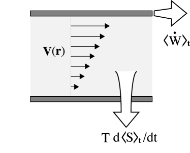
Figure 1: Schematic illustration of the power $\langle\dot{W}\rangle_{t}$ required to sustain the shear flow and the house-keeping heat $T[d\langle S\rangle_{t}/dt]$. In this illustration the power $\langle\dot{W}\rangle_{t}$ is represented as the power to move the upper boundary of the shearing system. This power supplies the energy to sustain the shear flow state, which is eliminated from the system as the house-keeping heat.

In steady flow systems, the energy added to the system by the work needed to sustain the flow must be eliminated from the system as heat Eva83 . This type of heat is called the ”house-keeping heat”, and its special role has been emphasized in the construction of a non-equilibrium steady state thermodynamics Ono98 ; Hat01 . Fig. 1 is a schematic illustration of the power $\langle\dot{W}\rangle_{t}$ required to sustain the shear flow and the house-keeping heat. Now we estimate this house-keeping heat from the non-equilibrium canonical distribution approach. For this purpose we introduce the non-equilibrium entropy $\langle S\rangle_{t}$ as the ensemble average of $S(\mbox{\boldmath$\bf\Gamma$})$ by the distribution $\tilde{f}(\mbox{\boldmath$\bf\Gamma$},t)$. Note that $S(\mbox{\boldmath$\bf\Gamma$})$ is defined by Eq. (21), and was already used as the observable corresponding to the entropy in Eq. (23). A similar kind of entropy to $\langle S\rangle_{t}$ was used in Refs. Mor56 ; Mor58 for a different form of the distribution $f(\mbox{\boldmath$\bf\Gamma$})$. Using Eq. (LABEL:GenerShearCanon2) the entropy $\langle S\rangle_{t}$ is represented as

$$\langle S\rangle_{t} = -\int d\mbox{\boldmath$\bf\Gamma$}f(\mbox{\boldmath$\bf\Gamma$})\ln\left\{\tilde{f}(\mbox{\boldmath$\bf\Gamma$},-t+2t_{0})\right\}$$ (54)

$$= \overline{S}+\beta\gamma\mathcal{V}\int_{t_{0}}^{-t+2t_{0}}ds\overline{\tilde{P}_{xy}(\mbox{\boldmath$\bf\Gamma$},-s+2t_{0})}$$

$$= \overline{S}-\beta\gamma\mathcal{V}\int_{t_{0}}^{t}ds\left\langle P_{xy}\right\rangle_{s}$$

Therefore the house-keeping heat $T[d\langle S\rangle_{t}/dt]$ at time $t$ is given by

$$T\frac{d\langle S\rangle_{t}}{dt} = -\gamma\mathcal{V}\left\langle P_{xy}\right\rangle_{t}$$ (55)

$$= \langle\dot{W}\rangle_{t}.$$ (56)

This is the balance equation to show that the power needed to sustain the shear flow must be equal to the house-keeping heat. Using Eqs. (50), (55) and (56), the house-keeping heat and the ensemble averaged power $\langle\dot{W}\rangle_{t}$ to sustain the shear flow is connected to the viscosity $\eta$ as $T[d\langle S\rangle_{t}/dt]=\langle\dot{W}\rangle_{t}=\mathcal{V}\eta\gamma^{2}+\mathcal{O}(\gamma^{3})$.

The entropy $\langle S\rangle_{t}$ satisfies the inequality

$$\langle S\rangle_{t}\geq\langle S\rangle_{t_{0}}=\overline{S}$$ (57)

at any time $t\;(>t_{0})$. The detail of the derivation of the inequality (57) is given in Appendix C. Noting that $\langle S\rangle_{t}-\langle S\rangle_{t_{0}}=\int_{t_{0}}^{t}dt[d\langle S\rangle_{t}/dt]$ and assuming that $d\langle S\rangle_{t}/dt$ is time-independent in a steady state, we obtain

$$\frac{d\langle S\rangle_{t}}{dt}\geq 0$$ (58)

This is the expression of the second law of thermodynamics in the non-equilibrium canonical distribution approach. The inequality (58) means simply that the shear flow system produces a positive house-keeping heat constantly in time. In this sense, the total entropy production $\langle S\rangle_{t}-\langle S\rangle_{t_{0}}$ diverges as time $t$ go to infinity, because the total amount of heat produced by the steady visco-elastic shear flow in the infinite time interval is infinite noteIV1 . In other words, the system is kept as a non-equilibrium steady state by discharging an amount of entropy constantly, which is transferred from the external work. Therefore the inequality (58) must be distinguished from another type of second law of thermodynamics meaning that an entropy increases in time and approaches to a stable value in a relaxation process. This type of the second law of thermodynamics, or the thermodynamical stability condition, will be discussed in Sec. V.2. By combining the inequality (58) and $T>0$ with Eqs. (55) and (56) we have

$$\frac{\langle\dot{W}\rangle_{\infty}}{\mathcal{V}}=-\gamma\left\langle P_{xy}(\mbox{\boldmath$\bf\Gamma$})\right\rangle_{\infty}\geq 0.$$ (59)

Namely the averaged power $\langle\dot{W}\rangle_{\infty}$ needed to sustain the shear flow must be positive (or zero). This is one of the results, which can be checked by numerical simulation, as will actually shown in Sec. VI.1. It may be noted that the inequality (59) implies the non-negativity of the viscosity $\eta$ as a special case.

V Thermodynamics for Shear Flow Systems

As discussed in Sec. IV.4, the factor $\exp\{\gamma\mathcal{V}\int_{t_{0}}^{t}ds\tilde{P}_{xy}(\mbox{\boldmath$\bf\Gamma$},-s+2t_{0})\}$, which gives the difference between the distribution $\tilde{f}(\mbox{\boldmath$\bf\Gamma$},t)$ and the canonical distribution $f(\mbox{\boldmath$\bf\Gamma$})$, includes the effect of the work needed to sustain the shear flow, or the house-keeping heat. On the other hand, the expression for the first law of thermodynamics proposed by Evans and Hanley does not include this effect (Otherwise it must include time-dependent terms for the sustaining work and the house-keeping heat.). Moreover, Ref. Hat01 emphasized that we must subtract the contribution of the house-keeping heat from the entropy in order to obtain an expression for the first law of thermodynamics for steady states. Equation (54) implies that the entropy minus the contribution from the house-keeping heat is given by $\langle S\rangle_{t}-\int_{t_{0}}^{t}ds[d\langle S\rangle_{s}/ds]=\langle S\rangle_{t}+\beta\gamma\mathcal{V}\int_{t_{0}}^{t}ds\langle P_{xy}(\mbox{\boldmath$\bf\Gamma$})\rangle_{s}=\overline{S}$, which is the entropy defined through the canonical distribution $f(\mbox{\boldmath$\bf\Gamma$})$, not through the distribution $\tilde{f}(\mbox{\boldmath$\bf\Gamma$},t)$. For these reasons, (although it may not be impossible to construct a non-equilibrium steady state thermodynamics explicitly including the effect of the house-keeping heat) in this section we construct a shear flow thermodynamics based on the canonical distribution $f(\mbox{\boldmath$\bf\Gamma$})$ excluding the effect of the house-keeping heat, and show that it is consistent with the Evans-Hanley thermodynamics.

V.1 First Law of Thermodynamics for Shear Flows

As the first thermodynamic property of the shear flow system, we consider the first law of thermodynamics. Its derivation is quite similar to that for the rotating system discussed in Sec. III.2, so it is given rather briefly.

In the shear flow system, the entropy $\overline{S}$ is given by Eq. (22) or

$$\overline{S}=\ln\Xi+\beta\left[\overline{H^{(ine)}}-\gamma\overline{Q}\right]$$ (60)

using the canonical distribution (42). As in the rotating system, the free energy $F^{(mov)}$ in the moving frame $\mathcal{F}^{(mov)}$ is defined by Eq. (24), and is connected to the partition function $\Xi$ by Eq. (25). (Here, it may be noted that the free energy $F^{(mov)}$ can also be expressed as $F^{(mov)}=\langle H^{(mov)}(\mbox{\boldmath$\bf\Gamma$})\rangle_{t}-T\langle S\rangle_{t}$ using the averaged energy $\langle H^{(mov)}(\mbox{\boldmath$\bf\Gamma$})\rangle_{t}$ and entropy $\langle S\rangle_{t}$ related to the distribution $\tilde{f}(\mbox{\boldmath$\bf\Gamma$},t)$ which includes information about the house-keeping heat.) Using this free energy $F^{(mov)}$ we obtain Eqs. (29) and

$$\frac{\partial\left[\beta F^{(mov)}\right]}{\partial\gamma}=-\frac{\partial\ln\Xi}{\partial\gamma}=-\beta\overline{Q}$$ (61)

which are equivalent to $d[\beta F^{(mov)}]=\overline{H^{(mov)}}d\beta-\beta\overline{Q}d\gamma$. Therefore we obtain

$$dF^{(mov)}=-\overline{S}dT-\overline{Q}d\gamma,$$ (62)

noting Eq. (24). Using the relations $F^{(ine)}=F^{(mov)}-\gamma\overline{Q}$, $\overline{H^{(mov)}}=F^{(mov)}+T\overline{S}$ and $\overline{H^{(ine)}}=F^{(ine)}+T\overline{S}$ we also obtain

$$dF^{(ine)}=-\overline{S}dT+\gamma d\overline{Q},$$ (63)

$$d\overline{H^{(mov)}}=Td\overline{S}-\overline{Q}d\gamma,$$ (64)

$$d\overline{H^{(ine)}}=Td\overline{S}+\gamma d\overline{Q}.$$ (65)

The two energies $\overline{H^{(ine)}}$ and $\overline{H^{(mov)}}$ in the different frames are connected by a Legendre transformation, namely $\overline{H^{(ine)}}=\overline{H^{(mov)}}-\gamma\;\partial\overline{H^{(mov)}}/\partial\gamma|_{\overline{S}}$, as well as the two free energies in the different frames. It is clear that the Evans-Hanley expression (1) for the first law of shear flow thermodynamics is the relation (64) where $\mathcal{E}=\overline{H^{(mov)}}$ and $\xi=-\overline{Q}$.

V.2 Thermodynamic Stability Conditions for Shear Flows

As the second thermodynamical property of the shear flow system, although we omitted to discuss it in Sec. III.2 for the rotating system, we consider a stability condition for shear flow note3 .

We consider a small part $\mathcal{A}$ of the macroscopic shear flow system, in which averages of energy, entropy and Helfand’s moment of viscosity in the inertial frame $\mathcal{F}^{(ine)}$ are given by $\overline{H^{(ine)}}$, $\overline{S}$ and $\overline{Q}$, respectively. The other part $\mathcal{R}$ of the system, which is much bigger than the system $\mathcal{A}$ and is called the ”environment” or ”reservoir”, has the thermodynamical values $T_{0}$, $\overline{S}_{0}$ and $\gamma_{0}$ of the temperature, the entropy and the shear rate, respectively. Now, we consider moving an infinitesimal amount of energy as heat $-T_{0}d\overline{S}_{0}$ from the reservoir $\mathcal{R}$ into the small system $\mathcal{A}$. In this process the total entropy must increase: $d\overline{S}+d\overline{S}_{0}\geq 0$. By combining this inequality with the first law of thermodynamics $d\overline{H^{(ine)}}=-T_{0}d\overline{S}_{0}+\gamma_{0}d\overline{Q}$ based on Eq. (65), we have $d\overline{H^{(ine)}}-T_{0}d\overline{S}-\gamma_{0}d\overline{Q}=d(\overline{H^{(ine)}}-T_{0}\overline{S}-\gamma_{0}\overline{Q})\leq 0$, using the fact that the reservoir $\mathcal{R}$ is so big that $T_{0}$ and $\gamma_{0}$ do not change in this process. This inequality means that the quantity $\overline{H^{(ine)}}-T_{0}\overline{S}-\gamma_{0}\overline{Q}$ always decreases and reaches a minimum at a stable state. In other words, if we force a change to the values of $\overline{H^{(ine)}}$, $\overline{S}$ and $\overline{Q}$ at the stable point by $\delta\overline{H^{(ine)}}$, $\delta\overline{S}$ and $\delta\overline{Q}$, respectively, then the inequality $\delta\overline{H^{(ine)}}-T_{0}\delta\overline{S}-\gamma_{0}\delta\overline{Q}\geq 0$ must be satisfied as the stability condition for the shear flow system. This simply leads to

$$\delta^{2}\overline{H^{(ine)}}\geq 0$$ (66)

for any infinitesimal deviations $\delta\overline{S}$ and $\delta\overline{Q}$. By a well known technique used in thermodynamics (See, for example, Ref. Lan59 or Appendix D.), the condition (66) is equivalent to

$$\left.\frac{\partial\overline{S}}{\partial T}\right|_{\overline{Q}}>0,$$ (67)

$$\left.\frac{\partial\overline{Q}}{\partial\gamma}\right|_{T}>0.$$ (68)

The condition (67) simply means that the specific heat at constant $\overline{Q}$ is always positive at a positive temperature $T$. To understand the condition (68) we note

$$\left.\frac{\partial\overline{Q}}{\partial\gamma}\right|_{T}=\beta\left(\overline{Q^{2}}-\overline{Q}^{2}\right)$$ (69)

as shown in Appendix D. Therefore, combining Eq. (69) with the inequality (68) we obtain

$$\overline{Q^{2}}-\overline{Q}^{2}>0.$$ (70)

Namely, the stability condition (69) means the positivity of the correlation function for Helfand’s moment $Q(\mbox{\boldmath$\bf\Gamma$})$ of viscosity.

Based on Eq. (1), Evans and Hanley claimed the inequality $\partial\xi/\partial\gamma|_{T}>0$ as a stability condition for shear flows Han82 ; Eva80b . This inequality is incompatible with the inequality (68) in the case of $\xi=-\overline{Q}$. This difference comes basically from the fact that they discussed a thermodynamic stability condition using the energy $\overline{H^{(mov)}}$, whereas we discussed it using the energy $\overline{H^{(ine)}}$. Obviously the correlation function of $Q$ cannot be negative because of $\overline{Q^{2}}-\overline{Q}^{2}=\overline{(Q-\overline{Q})^{2}}\geq 0$, so noting Eq. (69) we cannot justify the stability condition claimed by Evans and Hanley in the canonical distribution approach.

V.3 Relations Between Canonical Averages

So far we have introduced two types of canonical average $\overline{X}$ and $\langle X\rangle_{t}$, and in Sec. VI we introduce the usual time average. It is very important to distinguish between these averages. The thermodynamic relations discussed in Secs. V.1 and V.2 are the relations for the ensemble average $\overline{X}$ of observable $X(\mbox{\boldmath$\bf\Gamma$})$ using the canonical distribution $f(\mbox{\boldmath$\bf\Gamma$})$. On the other hand in numerical simulations using the Sllod equations with an isokinetic thermostat (as in Sec. VI), the values obtained are the mixed ensemble-time average $\langle X\rangle_{t}$ for the distribution $\tilde{f}(\mbox{\boldmath$\bf\Gamma$},t)$ in the limit $t\rightarrow\infty$. Therefore it is important to obtain an explicit relation between these two different ensemble averages.

For any function $X(\mbox{\boldmath$\bf\Gamma$})$ the relation between the two ensemble averages $\overline{X}$ and $\langle X\rangle_{\infty}$ is

$$\langle X\rangle_{\infty}$$

$$=\overline{X}-\beta\gamma\mathcal{V}\int_{t_{0}}^{\infty}dt\;\overline{\left[\tilde{X}(\mbox{\boldmath$\bf\Gamma$},t)-\overline{X}\right]\Bigl{[}P_{xy}(\mbox{\boldmath$\bf\Gamma$})-\overline{P_{xy}}\;\Bigr{]}}$$

(71)

where $\tilde{X}(\mbox{\boldmath$\bf\Gamma$},t)\equiv\exp\{i\hat{L}^{(ine)}(t-t_{0})\}X(\mbox{\boldmath$\bf\Gamma$})$. The derivation of Eq. (71) is given in Appendix E. A similar equation for the canonical distribution approach using the Sllod equations is shown in Ref. Eva87a .

From relation (71), if the fluctuation $\tilde{X}(\mbox{\boldmath$\bf\Gamma$},t)-\overline{X}$ of $X$ is weakly correlated to the shear stress $P_{xy}(\mbox{\boldmath$\bf\Gamma$})$, then the ensemble average $\overline{X}$ can be nicely approximated by the average $\langle X\rangle_{\infty}$. However one must notice that the justification for such an approximation strongly depends on the quantity $X$ we consider. A typical example is the case of $X=P_{xy}(\mbox{\boldmath$\bf\Gamma$})$, in which we must not neglect the second term on the right-hand side of Eq. (71), because in this case the first term on the right-hand side of Eq. (71) is zero, namely $\overline{P_{xy}}=0$, as shown in Appendix A. One should also notice that the second term in Eq. (71) is small near equilibrium, because it includes the non-equilibrium parameter $\gamma$ as a factor.

VI Numerical Simulations of Shear Flow

In this section we show numerical results for some quantities which have appeared in the preceding sections IV and V, and check the results obtained there.

For this numerical calculation we use a two-dimensional square system consisting of $N$ particles with a square shape and side length $L(=\sqrt{\mathcal{V}})$. The particle-particle interaction is given by the isotropic soft-core pair-potential

$$\phi(r)=\left\{\begin{array}[]{ll}\kappa\left(\frac{1}{r^{12}}-\frac{1}{r_{0}^{12}}\right)&\mbox{in}\;\;r<r_{0}\\ 0&\mbox{in}\;\;r\geq r_{0}\end{array}\right.$$ (74)

with a positive constants $r_{0}=1.5$ and $\kappa=1$. The particle number density $\rho\equiv N/\mathcal{V}$ is $0.8$. The mass $m$ of the particle and the kinetic temperature $T$ are both chosen as $1$. The number of particles is $N=450$, except in Sec. VI.4 in which the $N$-dependence of a quantity will be discussed. We use the Sllod equations with Lees-Edwards boundary conditions and the isokinetic thermostat so that the kinetic temperature (given by Eq. (45)) is kept constant Eva90a . (This dynamics is explained in Appendix B more explicitly.) A predictor-corrector method Gea71 of 4-th order is used to carry out these numerical simulations with time step of $\Delta t=0.001$. In this algorithm the sum of the ”thermal momentum” $\tilde{\mathbf{p}}_{j}\equiv\mathbf{p}_{j}-m\mathbf{V}(\mathbf{q}_{j})$ is zero in the both coordinate directions.

We use the notation $\langle X\rangle$ for the time-averaged value of any quantity $X$ given by this numerical simulation. To calculate this average we used data over more than $10^{6}$ time steps omitting the first $10^{4}$ time steps. (We checked that $10^{4}$ time steps is much longer than the relaxation time of the time-correlation function for the thermal momentum.) This should correspond to the ensemble average $\langle X\rangle_{\infty}$ used so far. This is supposed by the fact that we can calculate the viscosity from the time-average $\langle P_{xy}\rangle$ in this simulation, based on Eq. (50) assuming $\langle P_{xy}\rangle_{\infty}=\langle P_{xy}\rangle$. We calculate $\gamma$-dependences of three quantities: $\langle P_{xy}\rangle$, $\langle Q\rangle$ and $\langle Q^{2}\rangle$. We use $\langle P_{xy}\rangle$ to discuss the power to sustain the flow and the house-keeping heat given by Eq. (55). The quantities $\langle Q\rangle$ and $\langle Q^{2}\rangle$ are used to discuss the behavior of Helfand’s moment of viscosity and the thermodynamic stability condition (68). Here, it is assumed that the quantities $Q$ and $P_{xy}$ are not strongly correlated with each other because of the relation (41), and in the case of $X=Q$ or $Q^{2}$ the second term of the right-hand side of Eq. (71) may be small compared to the first term in the small shear rate case. This implies that the behavior of the time-averages of Helfand’s moment of viscosity and its correlation function are not so different from the ones for $\overline{Q}$ and $\overline{Q^{2}}-\overline{Q}^{2}$, respectively, near equilibrium.

VI.1 Work Needed to Sustain the Shear Flow

The first numerical result is for the power $\dot{W}/\mathcal{V}$ per unit volume ($\mathcal{V}=562.499\cdots$) for the work required to sustain the shear flow, or equivalently in a quantitative sense, the house-keeping heat per unit volume. It is given as the time-average of $\dot{W}/\mathcal{V}\equiv-\gamma P_{xy}(\mbox{\boldmath$\bf\Gamma$})$, based on Eqs. (55) and (56). Figure 2 shows the shear rate $\gamma$ dependence of the time-averaged power $\langle\dot{W}\rangle/\mathcal{V}$ per volume. The inset is the same graph except showing it in a wider shear rate region. (Note that we used a linear-log scale in this inset, whereas we use a linear-linear scale for the main figure.) Following from the inequality (59), the power to sustain the flow shown in Fig. 2 is always positive (or zero).

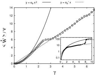
Figure 2: The averaged power $\langle\dot{W}\rangle/\mathcal{V}$ divided by volume $\mathcal{V}$ needed to sustain the shear flow, as a function of shear rate $\gamma$ as a linear-linear plot. The solid line is the fit to a quadratic function and the dashed line is the fit to a linear function (valid for $\gamma>3$). Inset: the same graph as a linear-log plot including a wider range of $\gamma$.

It may be noted that the averaged power $\langle\dot{W}\rangle$ needed to sustain the shear flow should be an even function of $\gamma$, because it should be invariant under a change of sign of the shear rate $\gamma$. In Fig. 2 we fitted the numerical data to a quadratic function $y=\alpha_{P}x^{2}$ with the fitting parameter $\alpha_{P}=1.51309$. Near equilibrium $\gamma<0.5$, the graph is nicely fitted by this quadratic function.

As the shear rate increases, a region in which the value of $\langle P_{xy}(\mbox{\boldmath$\bf\Gamma$})\rangle$ is almost independent of $\gamma$, (namely the region fitted by a linear function $y=\alpha_{P}^{\prime}x$ with the fitting parameter $\alpha_{P}^{\prime}=2.00005$), appears Woo84 , and after that the region the string phase appears Erp84 ; Woo84 ; Hey85 (the region $\gamma>8$ approximately in the inset to Fig. 2). The string phase can be checked not only by the string-type arrangement of particle positions but also by strong time-oscillating behavior of the time-correlation functions for quantities such as the potential energy, the shear stress and so on Hey85 .

For isokinetic thermostat, the house-keeping heat is also given as the time-average of the thermostat term (the term $-\alpha(t)\mathbf{p}^{\prime}_{j}(t)$ explained in Appendix B). We checked numerically that this quantity is equal to the time-average of $-\gamma P_{xy}(\mbox{\boldmath$\bf\Gamma$})$.

VI.2 Helfand’s Moment of Viscosity

As a second numerical result, Fig. 3 shows the graph of the time-average $\langle Q\rangle/\mathcal{V}$ of the Helfand’s moment of viscosity per unit volume $\mathcal{V}$ as a function of shear rate $\gamma$. It (almost) takes the value $0$ at the equilibrium $\gamma=0$, and increases linearly as a function of $\gamma$. In this figure we also give a fit to a linear function $y=\alpha_{Q}\gamma$, with the parameter value $\alpha_{Q}=150.043$.

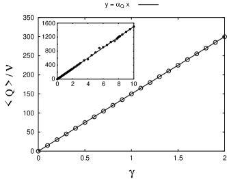
Figure 3: Time-average $\langle Q\rangle/\mathcal{V}$ of Helfand’s moment of viscosity divided by volume $\mathcal{V}$ as a function of shear rate $\gamma$. The solid line is the fit to a linear function. Inset: the same graph including a wider range of $\gamma$.

To explain this linear behavior for Helfand’s moment of viscosity as a function of shear rate, we simply note that

$$\left\langle Q\right\rangle=\sum_{j=1}^{N}\left\langle q_{jy}\tilde{p}_{jx}\right\rangle+\gamma\sum_{j=1}^{N}\left\langle q_{jy}^{2}\right\rangle$$ (75)

with the $x$-component $\tilde{p}_{jx}\equiv p_{jx}-\gamma q_{jy}$ of the thermal momentum of the $j$-th particle. Our numerical calculations show that the value of the first term of the right-hand side of Eq. (75) is extremely small (or zero) compared to the value of its second term, namely $\sum_{j=1}^{N}\langle q_{jy}\tilde{p}_{jx}\rangle\approx 0$. Moreover, using a homogeneous continuum assumption for the fluid, the value of the quantity $\sum_{j=1}^{N}\langle q_{jy}^{2}\rangle$ appearing in the second term of the right-hand side of Eq. (75) can be estimated as $\sum_{j=1}^{N}\langle q_{jy}^{2}\rangle\approx NL^{-1}\int_{0}^{L}dyy^{2}=NL^{2}/3$. These estimations lead to $\langle Q\rangle/\mathcal{V}\approx(N/3)\gamma=150\gamma$, which explains the value of the fitting parameter $\alpha_{Q}$.

The time-averaged Helfand’s moment $\langle Q\rangle$ of viscosity should be at least an odd function of shear rate $\gamma$, because the infinitesimal deviation $\gamma d\overline{Q}$ giving the energy change $d\overline{H^{(ine)}}$ in the inertial frame by Eq. (65) must be invariant under the change of sign of the shear rate. It may be noted that this linear dependence for the time-average of Helfand’s moment $Q$ of viscosity with respect to shear rate is satisfied not only in the near equilibrium region but also even in the string phase region, shown in the inset to Fig. 3, possibly because the Sllod equations are a homogenous shear algorithm.

It may be noted that in our simulations Helfand’s moment of viscosity can be generally changed discontinuously in time, when a particle steps over a boundary in the direction orthogonal to the global shear flow. However it should be a small boundary effect which can be neglected in the thermodynamic limit $N\rightarrow\infty$ and $\rho=const$, and our numerical calculations gave a good convergence for the long time-average of Helfand’s moment of viscosity.

VI.3 Correlation Function for Helfand’s Moment of Viscosity

As the last example, Fig. 4 shows the shear rate dependence of the correlation function $(\langle Q^{2}\rangle-\langle Q\rangle^{2})/\mathcal{V}$ of Helfand’s moment of viscosity divided by the volume $\mathcal{V}$. This figure shows that this correlation function is always positive at least for $\gamma<10$, following the thermodynamic stability condition (68).

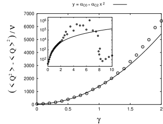
Figure 4: Correlation function $(\langle Q^{2}\rangle-\langle Q\rangle^{2})/\mathcal{V}$ of Helfand’s moment of viscosity divided by volume $\mathcal{V}$ as a function of shear rate $\gamma$ in a linear-linear plot. The solid line is the fit to a quadratic function. The inset: the same graph except for that it includes a wider region of $\gamma$ and is a linear-log plot.

The correlation function for Helfand’s moment of viscosity should be an even function of the shear rate. Noting this point, in the small shear rate region of Fig. 4 we give the fit of numerical data to the function $y=\alpha_{C0}+\alpha_{C2}x^{2}$ with the fitting parameter values $\alpha_{C0}=46.749$ and $\alpha_{C2}=1349.38$. The graph is nicely fitted by this quadratic function in the small shear rate region. This point may be explained by noting

$$\left\langle Q^{2}\right\rangle-\left\langle Q\right\rangle^{2} \approx \sum_{j=1}^{N}\sum_{k=1}^{N}\left\langle q_{jy}q_{ky}\tilde{p}_{jx}\tilde{p}_{kx}\right\rangle$$

$$+\gamma^{2}\sum_{j=1}^{N}\sum_{k=1}^{N}\left(\left\langle q_{jy}^{2}q_{ky}^{2}\right\rangle-\left\langle q_{jy}^{2}\right\rangle\left\langle q_{ky}^{2}\right\rangle\right)$$

using the thermal momentum component $\tilde{p}_{jx}$. Here we assumed that the time-average of the linearly dependent terms for the thermal momentum can be neglected. As the two terms $\sum_{j=1}^{N}\sum_{k=1}^{N}\langle q_{jy}q_{ky}\tilde{p}_{jx}\tilde{p}_{kx}\rangle$ and $\sum_{j=1}^{N}\sum_{k=1}^{N}\sum_{j=1}^{N}\langle q_{jy}^{2}q_{ky}^{2}\rangle$ can be considered $\gamma$-independent, the correlation $\langle Q^{2}\rangle-\langle Q\rangle^{2}$ can be fitted by a quadratic function of $\gamma$.

In the inset to Fig. 4, we give the shear rate dependence of the time-average of the correlation function for Helfand’s moment of viscosity per unit volume $\mathcal{V}$ in a much wider region of shear rate in a linear-log scale. (Note that we used a linear-linear scale in the main figure of Fig. 4.) It should be noted that a rapid drop of the value of this correlation function occurs in the string phase region. In the intermediate region, which is approximately the region $2.5<\gamma<8$ in Fig. 4, between the region fitted by the quadratic function of $\gamma$ and the string phase region, fluctuations in the value $\langle Q^{2}\rangle-\langle Q\rangle^{2}$ become much larger than in the other regions, and their values in Fig. 4 are less reliable.

VI.4 Remarks in Connection with the Isokinetic Thermostat Dynamics and the Canonical Distribution Approach

Sllod dynamics with the isokinetic thermostat used in this section has been used very frequently to simulate shear flows. It is supposed to reproduce the value of shear stress predicted by a canonical distribution approach Mor88 , and succeeded even to reproduce some real experimental values Mar01a . However one must notice that strictly speaking the time-average from Sllod dynamics with the isokinetic thermostat does not always reproduce the ensemble average for the non-equilibrium canonical distribution used in this paper, even in the equilibrium state where $\gamma=0$ after taking the thermodynamic limit $N\rightarrow\infty$ (and $\rho=const$). Now we discuss a couple of examples illustrating these ensemble differences.

First, in the numerical simulations used in this section the sum of the thermal momentum $\tilde{\mathbf{p}}_{j}\equiv(\tilde{p}_{jx},\tilde{p}_{jy})\equiv\mathbf{p}_{j}-m\mathbf{V}(\mathbf{q}_{j})$ over the particle number $j$ in each direction is zero at all time, meaning that there is a constraint on the values of the thermal momenta, that is $\sum_{j=1}^{N}\tilde{p}_{jx}=0$. On the other hand, in the canonical distribution approach all components of momenta can be treated as independent variables. This difference, for example, causes the different averaged values for $\sum_{j=1}^{N}\sum_{k=1}^{N}\langle\tilde{p}_{jx}\tilde{p}_{kx}\rangle$ and $\sum_{j=1}^{N}\sum_{k=1}^{N}\overline{\tilde{p}_{jx}\tilde{p}_{kx}}$. Actually the value of $\sum_{j=1}^{N}\sum_{k=1}^{N}\langle\tilde{p}_{jx}\tilde{p}_{kx}\rangle=\langle(\sum_{j=1}^{N}\tilde{p}_{jx})(\sum_{k=1}^{N}\tilde{p}_{kx})\rangle$ is zero as each bracketed sum is individually zero. The value of $\sum_{j=1}^{N}\sum_{k=1}^{N}\overline{\tilde{p}_{jx}\tilde{p}_{kx}}$ however, is given by $mNT$ in the canonical distribution because of $\overline{\tilde{p}_{jx}\tilde{p}_{kx}}=mT\delta_{jk}$.

Second, the isokinetic thermostat used in the simulations of this section keeps the kinetic energy constant so that the distribution function for the kinetic energy is given by a delta function. This is different from the distribution of kinetic energy derived from the canonical distribution, because there is always a non-zero fluctuation of the kinetic energy around its mean value in the canonical distribution. Refs. Eva83b ; Eva84 tried to modify the canonical distribution to give consistency with the isokinetic thermostat, but it is not obvious that we can justify the shear flow thermodynamics based on such a modified canonical distribution.

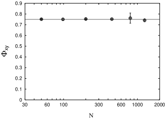
Figure 5: Time-averaged quantity $\Phi_{xy}\equiv|\tilde{\Psi}_{xy}-\bar{\Psi}_{xy}|/\bar{\Psi}_{xy}$ as a function of particle number $N$ for Sllod dynamics with an isokinetic thermostat in a square at equilibrium $\gamma=0$ with the particle density $\rho=0.8$ as a log-linear plot. Here $\tilde{\Psi}_{xy}$ and $\bar{\Psi}_{xy}$ are defined by $\tilde{\Psi}_{xy}\equiv\sum_{j=1}^{N}\sum_{k=1}^{N}\langle q_{jy}q_{ky}\tilde{p}_{jx}\tilde{p}_{kx}\rangle|_{\gamma=0}$ and $\bar{\Psi}_{xy}\equiv mT\sum_{j=1}^{N}\langle q_{jy}^{2}\rangle|_{\gamma=0}$, respectively. The length of error bars in this figure is given by $2|\Phi_{xy}-\Phi_{yx}|$. The solid line is the value $3/4$, which is explained in the text.

As a concrete example of these ensemble differences, let’s consider the first term $\tilde{\Psi}_{xy}\equiv\sum_{j=1}^{N}\sum_{k=1}^{N}\langle q_{jy}q_{ky}\tilde{p}_{jx}\tilde{p}_{kx}\rangle|_{\gamma=0}$ appearing on the right-hand side of Eq. (LABEL:HelfaCorri) at equilibrium $\gamma=0$. Assuming that the variables $q_{jy}$ and $\tilde{p}_{jx}$ are independent, and that $\langle q_{jy}q_{ky}\rangle$ only depends upon whether $j=k$ or $j\neq k$, then

$$\sum_{j=1}^{N}\sum_{k=1}^{N}\left\langle q_{jy}q_{ky}\tilde{p}_{jx}\tilde{p}_{kx}\right\rangle$$

$$\approx\left\langle q_{1y}^{2}\right\rangle\sum_{j=1}^{N}\left\langle\tilde{p}_{jx}^{2}\right\rangle+\left\langle q_{1y}q_{2y}\right\rangle\sum_{j=1}^{N}\sum_{k=1(k\neq j)}^{N}\left\langle\tilde{p}_{jx}\tilde{p}_{kx}\right\rangle$$ (77)

If $q_{1y}$ is uniformly distributed between $0$ and $L$ then $\langle q_{1y}^{2}\rangle\approx L^{2}/3$ and $\langle q_{1y}q_{2y}\rangle\approx L^{2}/4$. The difference between $\bar{\Psi}_{xy}$ and $\tilde{\Psi}_{xy}$ can be calculated as $\overline{\tilde{p}_{jx}\tilde{p}_{kx}}=0$ in $j\neq k$ for the canonical average, whereas for the time average $\sum_{j\neq k}\langle\tilde{p}_{jx}\tilde{p}_{kx}\rangle=-\sum_{j=1}^{N}\langle\tilde{p}_{jx}^{2}\rangle$. It follows that $\bar{\Psi}_{xy}\approx mNTL^{2}/3$ and $\tilde{\Psi}_{xy}\approx mNTL^{2}/12$, so $\Phi_{xy}\equiv|\tilde{\Psi}_{xy}-\bar{\Psi}_{xy}|/\bar{\Psi}_{xy}\approx 3/4$. Figure 5 is the graph of the normalized difference $\Phi_{xy}$ as a function of system size $N$ for square systems at fixed density $\rho=0.8$ in numerical simulations. The length of error bars in this figure is given by $2|\Phi_{xy}-\Phi_{yx}|$ which must be zero in the square cases. Figure 5 suggests that $\Phi_{xy}$ is in excellent agreement with the value of $3/4$ given above.

VII Conclusion and Remarks

In this paper we have discussed a canonical distribution approach to non-equilibrium steady flows for the purpose of constructing a steady state thermodynamics from solid statistical mechanical foundations. Using the Lagrangian technique of classical mechanics we introduced the energy in the moving frame by separating the velocity of the global steady flow. A canonical distribution based on this internal energy was introduced. As one application of this distribution, we showed that the well known thermodynamics of rotating systems can be derived from this canonical distribution. Our special concern in this canonical distribution approach was steady shear flows and their thermodynamics. Evans and Hanley proposed a first law of thermodynamics of the form $d\mathcal{E}=Td\mathcal{S}-\mathcal{Q}d\gamma$ relating energy $\mathcal{E}$, temperature $T$, entropy $\mathcal{S}$ and shear rate $\gamma$. Here we derived this shear flow thermodynamics based on our canonical distribution approach, and showed that the quantity $\mathcal{Q}$ is given by the average of Helfand’s moment of viscosity, the temperature $T$ is the kinetic temperature derived from the thermal kinetic energy, and $\mathcal{E}$ can be interpreted as an internal energy. The roles of the work required to sustain the shear flow and the heat removed to compensate it (the house-keeping heat) was emphasized in the justification of the linear response formula for viscosity, which is derived from our shear flow canonical distribution approach. We introduced a non-equilibrium entropy, and showed that it increases in time and the house-keeping heat based on this entropy has the same magnitude as the power needed to sustain the steady flow. This discussion led to the non-negativity of average of $-\gamma P_{xy}$ with the shear stress $P_{xy}$, meaning that the power needed to sustain the shear flow and the house-keeping heat is always non-negative. We discussed the thermodynamic stability condition for the shear flows, one of which is equivalent to the positivity of the correlation function of Helfand’s moment of viscosity. Our results were investigated in numerical simulations of two-dimensional many-particle systems with soft-core interactions, whose dynamics is determined by the Sllod equations with an isokinetic thermostat.

To construct the canonical distribution for shear flow, we used the analogy of shear flows and rotating systems. These two systems are steady flows whose magnitude is proportional to a component of position vector: the distance from the rotating axis in the rotating system, and the position component orthogonal to the flow in the shear system. Both systems also have clear parameters to characterize their currents: the angular velocity in the rotating system and the shear rate in the shear flow. On the other hand, we also emphasized some differences between these two systems. The biggest difference may be that the total angular momentum in the canonical distribution of the rotating system is time-independent, whereas Helfand’s moment of viscosity appearing the canonical distribution of the shear flow is not constant. This led to the necessity to consider the work needed to sustain the steady flow and the house-keeping heat in the shear flow system, and plays an essential role in the derivation of the response formula for viscosity.

One may easily notice that the canonical distribution approach discussed in this paper can be generalized to more general steady flows than the rotating system and the shear flow system. One of the restrictions in our canonical distribution approach is that we have to know the global velocity distribution $\mathbf{V}$ a priori. In this sense this approach is not appropriate to determine the global velocity distribution under some external constraints, etc. It is also crucial that we know a priori an external parameter that specifies the amount of the global flow, like the angular velocity or the the shear rate. This parameter is treated as a thermodynamic quantity in the expression for the first law of thermodynamics.

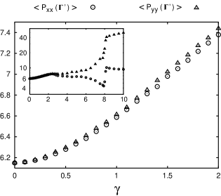
Figure 6: Time-averages of the diagonal components $\langle P_{xx}(\mbox{\boldmath$\bf\Gamma$}^{\prime})\rangle$ (circles) and $\langle P_{yy}(\mbox{\boldmath$\bf\Gamma$}^{\prime})\rangle$ (triangles) of the pressure tensor with the thermal phase space vector $\mbox{\boldmath$\bf\Gamma$}^{\prime}$ as functions of shear rate $\gamma$ in Sllod dynamics with an isokinetic thermostat in a linear-linear plot. The inset: the same graph except for including a wider region of shear rate and in a linear-log plot.

An important future problem in shear flow thermodynamics based on the canonical distribution approach is to discuss the pressure in this framework. Refs. Eva80a ; Eva80b ; Han82 ; Eva83 introduced the pressure $\mathcal{P}$ simply by adding the term $-\mathcal{P}d\mathcal{V}$ on the right-hand side of Eq. (1). For this term it was conjectured that the pressure $\mathcal{P}$ would be equal to the minimum eigenvalue of the pressure tensor Eva89 . However one should notice that non-equilibrium systems such as the shear flow system are not generally isotropic, so that the pressure defined by $-\partial\mathcal{E}/\partial\mathcal{V}$ may depend on which direction we change the volume $\mathcal{V}$. Actually, as shown in Fig. 6, the numerical simulations using Sllod dynamics in Sec. VI show that the time averages of $P_{xx}(\mbox{\boldmath$\bf\Gamma$}^{\prime})$ and $P_{yy}(\mbox{\boldmath$\bf\Gamma$}^{\prime})$ are different from each other at non-zero shear rate. (Here $\mbox{\boldmath$\bf\Gamma$}^{\prime}$ is the ”thermal phase space vector” introduced as the vector in which the momentum $\mathbf{p}_{j}$ in the phase space vector is replaced by the thermal momentum $\tilde{\mathbf{p}}_{j}\equiv\mathbf{p}_{j}-m\mathbf{V}(\mathbf{q}_{j})$.) Noting that usually the pressure is calculated by the arithmetic average of these time-averages (or ensemble averages), (See Ref. Eva90a , also Ref. Zub74 for its justification using the microcanonical distribution.), this suggests that if the pressures in the $x$ and the $y$-directions are given by averages of $P_{xx}(\mbox{\boldmath$\bf\Gamma$}^{\prime})$ and $P_{yy}(\mbox{\boldmath$\bf\Gamma$}^{\prime})$, respectively, then the pressure is direction-dependent in shear flow systems. The quantity $\langle P_{xx}(\mbox{\boldmath$\bf\Gamma$}^{\prime})\rangle-\langle P_{yy}(\mbox{\boldmath$\bf\Gamma$}^{\prime})\rangle$ is called the ”normal stress” and a non-zero value is one of the important properties of visco-elastic fluids Tsh89 ; Eva90a ; Que81 . Therefore it is important to understand whether such a property is compatible with the thermodynamical framework discussed in this paper, in other words, to discuss the first law of thermodynamics in which the averages $\overline{P_{xx}(\mbox{\boldmath$\bf\Gamma$}^{\prime})}$ and $\overline{P_{yy}(\mbox{\boldmath$\bf\Gamma$}^{\prime})}$ are included as the $x$ and $y$-components of the pressure, respectively. It may be noted that a similar question can be asked for rotating systems. We leave discussion of these points for the future.

As mentioned in Sec. V.3, the thermodynamic relations, (65) and (70) derived in this paper, are relations for the ensemble average (19) under the canonical distribution $f(\mbox{\boldmath$\bf\Gamma$})$. On the other hand the numerical calculations discussed in Sec. VI give the average (49) under the distribution $\tilde{f}(\mbox{\boldmath$\bf\Gamma$},\infty)$. Although these two averages are related by Eq. (71), it is still an open question to calculate the canonical average (19), required for the thermodynamic relations, from the dynamical evolved canonical average (49) in numerical calculations.

Originally, Evans and Hanley introduced their shear flow thermodynamics to discuss non-analytical properties of the pressure, viscosity and the internal energy as functions of the shear rate. Such non-analytical properties are predicted by mode-coupling theory Kaw73 ; Pom75 , and are supported by some numerical calculations Eva90a ; Eva80c ; Eva81 . However, recently some numerical works suggest that the shear rate dependence of the pressure is rather analytic near equilibrium, except at the triple point Mar01a ; Ge01 . Moreover, even at the triple point the non-analytic dependence of the pressure is not completely convincing Tra95 . It may also be noted that some theories, that predict an analytic dependence of the pressure and the viscosity with respect to the shear rate, have been proposed Jou01 ; Tra95 ; Que81 . In this sense it is still an interesting problem to discuss shear rate dependences of the pressure, the viscosity and so on using shear flow thermodynamics.

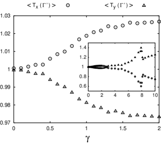
Figure 7: $x$-component $\langle T_{x}(\mbox{\boldmath$\bf\Gamma$}^{\prime})\rangle$ (circles) and $y$-component $\langle T_{y}(\mbox{\boldmath$\bf\Gamma$}^{\prime})\rangle$ (triangles) of the kinetic temperature with the thermal phase space vector $\mbox{\boldmath$\bf\Gamma$}^{\prime}$ as functions of shear rate $\gamma$ in the Sllod dynamics with the isokinetic thermostat. The inset: the same graph except for including a wider range of shear rate.

There are also questions about the numerical simulations of shear flow themselves, from the point of view of the canonical distribution approach. Some such problems were already mentioned in Sec. VI.4. As another potential problem, we mention the direction dependence of the thermal kinetic energy. To discuss this point we introduce the quantities $T_{x}(\mbox{\boldmath$\bf\Gamma$}^{\prime})$ and $T_{y}(\mbox{\boldmath$\bf\Gamma$}^{\prime})$ as $T_{k}(\mbox{\boldmath$\bf\Gamma$}^{\prime})\equiv(2/N)\sum_{j=1}^{N}\tilde{p}_{jk}^{2}/(2m)$ with the thermal momentum component $\tilde{p}_{jk}\equiv p_{jk}-mV_{k}(\textbf{q}_{j})$, where $V_{k}$ is the $k$-component of the global current density $\mathbf{V}$. The arithmetic average of ensemble averages of $\{T_{k}(\mbox{\boldmath$\bf\Gamma$}^{\prime})\}_{k}$ over the component $k$ gives the kinetic temperature, so we may interpret the quantity $T_{k}(\mbox{\boldmath$\bf\Gamma$}^{\prime})$ as the observable for the ”$k$-component of the temperature”. The canonical distribution approach discussed in this paper claims that the ensemble average $\overline{T_{k}(\mbox{\boldmath$\bf\Gamma$}^{\prime})}$ of the quantity $T_{k}(\mbox{\boldmath$\bf\Gamma$}^{\prime})$ is $k$-independent, in other words the kinetic temperature is direction-independent, although we should note a difference in the two averages $\overline{T_{k}(\mbox{\boldmath$\bf\Gamma$}^{\prime})}$ and $\langle T_{k}(\mbox{\boldmath$\bf\Gamma$}^{\prime})\rangle_{\infty}$. Figure 7 shows the graphs of $\langle T_{x}(\mbox{\boldmath$\bf\Gamma$}^{\prime})\rangle$ and $\langle T_{y}(\mbox{\boldmath$\bf\Gamma$}^{\prime})\rangle$ as functions of shear rate $\gamma$ from numerical simulations using the Sllod dynamics with an isokinetic thermostat, used in Sec. VI. This figure shows that the kinetic temperature is direction-dependent at least in large shear rate cases. As a topic related to this point, it may be noted that in the isokinetic thermostat the heat is removed from any component of kinetic energy of any particle uniformly. This gives great simplification in the formula and numerical calculations and keeps a similar dynamical structure to Hamiltonian dynamics leading to the numerical observation of the conjugate pairing rule for the Lyapunov spectrum Mor01 , but its physical justification as a mechanical thermostat is not completely convincing. For example, one may use other types of thermostats in which the heat is removed from the particles near the walls or from the kinetic energy component orthogonal to the walls Tro84 ; Pos89 . These different thermostats might give, for example, different values of $\langle T_{x}(\mbox{\boldmath$\bf\Gamma$}^{\prime})\rangle$ and $\langle T_{y}(\mbox{\boldmath$\bf\Gamma$}^{\prime})\rangle$ from the isokinetic thermostat. To check the shear flow thermodynamics for such types of thermostat remains an open problem.

Appendix A Response Formula for the Viscosity from the Canonical Distribution Approach

In this appendix we give a derivation of the linear response formula (51) for viscosity from the definition (50), as well as a derivation of Eq. (52). We also discuss the two kinds of nonlinear response formulas for $\left\langle P_{xy}(\mbox{\boldmath$\bf\Gamma$})\right\rangle_{\infty}$ with respect to the shear rate $\gamma$, one of which is a simple generalization of the formula (51).

First we note that the partition function $\Xi$ can be rewritten as

$$\Xi \equiv \int d\mbox{\boldmath$\bf\Gamma$}\exp\left\{-\beta H^{(mov)}(\mbox{\boldmath$\bf\Gamma$})\right\}$$ (78)

$$= \int d\mbox{\boldmath$\bf\Gamma$}\exp\left\{-i\hat{L}^{(ine)}(t-t_{0})\right\}$$

$$\hskip 14.22636pt\times\exp\left\{-\beta H^{(mov)}(\mbox{\boldmath$\bf\Gamma$})\right\}$$

$$= \int d\mbox{\boldmath$\bf\Gamma$}\exp\left\{-\beta H^{(mov)}(\mbox{\boldmath$\bf\Gamma$})\right\}$$

$$\hskip 14.22636pt\times\exp\left\{-\beta\gamma\mathcal{V}\int_{t_{0}}^{t}ds\tilde{P}_{xy}(\mbox{\boldmath$\bf\Gamma$},-s+2t_{0})\right\}\;\;\;$$

where we used the relations $\exp\{-i\hat{L}^{(ine)}(t-t_{0})\}1=1$, $(i\hat{L}^{(ine)})^{\dagger}=-i\hat{L}^{(ine)}$ ($\dagger$ meaning to take its Hermitian conjugate) and a similar derivation to that in Eq. (LABEL:GenerShearCanon2). Equation (78) means that both the distributions $f(\mbox{\boldmath$\bf\Gamma$})$ and $\tilde{f}(\mbox{\boldmath$\bf\Gamma$},t)$ are normalized with the same partition function $\Xi$. The partition function $\Xi$ given by Eq. (78) must be time-independent, so that we obtain

$$0 = \frac{\partial\Xi}{\partial t}$$ (79)

$$= -\beta\gamma\mathcal{V}\int d\mbox{\boldmath$\bf\Gamma$}\tilde{P}_{xy}(\mbox{\boldmath$\bf\Gamma$},-t+2t_{0})$$

$$\hskip 14.22636pt\times\exp\left\{-\beta H^{(mov)}(\mbox{\boldmath$\bf\Gamma$})\right\}$$

$$\hskip 14.22636pt\times\exp\left\{-\beta\gamma\mathcal{V}\int_{t_{0}}^{t}ds\tilde{P}_{xy}(\mbox{\boldmath$\bf\Gamma$},-s+2t_{0})\right\}$$

$$= -\beta\gamma\mathcal{V}\Xi\int d\mbox{\boldmath$\bf\Gamma$}\tilde{P}_{xy}(\mbox{\boldmath$\bf\Gamma$},-t+2t_{0})$$

$$\hskip 14.22636pt\times\exp\left\{-i\hat{L}^{(ine)}(t-t_{0})\right\}f(\mbox{\boldmath$\bf\Gamma$})$$

$$= -\beta\gamma\mathcal{V}\Xi\int d\mbox{\boldmath$\bf\Gamma$}\exp\left\{-i\hat{L}^{(ine)}(t-t_{0})\right\}$$

$$\hskip 14.22636pt\times P_{xy}(\mbox{\boldmath$\bf\Gamma$})f(\mbox{\boldmath$\bf\Gamma$})$$

$$= -\beta\gamma\mathcal{V}\Xi\overline{P_{xy}(\mbox{\boldmath$\bf\Gamma$})}$$

noting the definition of the average (19). From Eq. (79) we obtain Eq. (52), implying that the viscosity calculated from the canonical distribution $f(\mbox{\boldmath$\bf\Gamma$})$ is zero.

On the other hand, using the average (49) by the distribution $\tilde{f}(\mbox{\boldmath$\bf\Gamma$},t)$ given by Eq. (LABEL:GenerShearCanon2) we have

$$\left\langle P_{xy}(\mbox{\boldmath$\bf\Gamma$})\right\rangle_{\infty} = \lim_{t\rightarrow\infty}\int d\mbox{\boldmath$\bf\Gamma$}P_{xy}(\mbox{\boldmath$\bf\Gamma$})f(\mbox{\boldmath$\bf\Gamma$})\exp\left\{-\beta\gamma\mathcal{V}\int_{t_{0}}^{t}ds\tilde{P}_{xy}(\mbox{\boldmath$\bf\Gamma$},-s+2t_{0})\right\}$$ (80)

$$= \int d\mbox{\boldmath$\bf\Gamma$}P_{xy}(\mbox{\boldmath$\bf\Gamma$})f(\mbox{\boldmath$\bf\Gamma$})-\beta\gamma\mathcal{V}\int_{t_{0}}^{\infty}ds\int d\mbox{\boldmath$\bf\Gamma$}P_{xy}(\mbox{\boldmath$\bf\Gamma$})f(\mbox{\boldmath$\bf\Gamma$})\tilde{P}_{xy}(\mbox{\boldmath$\bf\Gamma$},-s+2t_{0})+\mathcal{O}(\gamma^{2})$$

$$= \overline{P_{xy}(\mbox{\boldmath$\bf\Gamma$})}-\beta\gamma\mathcal{V}\int_{t_{0}}^{\infty}ds\int d\mbox{\boldmath$\bf\Gamma$}P_{xy}(\mbox{\boldmath$\bf\Gamma$})f^{(eq)}(\mbox{\boldmath$\bf\Gamma$})\tilde{P}_{xy}(\mbox{\boldmath$\bf\Gamma$},-s+2t_{0})+\mathcal{O}(\gamma^{2})$$

$$= -\beta\gamma\mathcal{V}\int_{t_{0}}^{\infty}ds\int d\mbox{\boldmath$\bf\Gamma$}P_{xy}(\mbox{\boldmath$\bf\Gamma$})f^{(eq)}(\mbox{\boldmath$\bf\Gamma$})\exp\left\{-i\hat{L}^{(ine)}(s-t_{0})\right\}P_{xy}(\mbox{\boldmath$\bf\Gamma$})+\mathcal{O}(\gamma^{2})$$

$$= -\beta\gamma\mathcal{V}\int_{t_{0}}^{\infty}ds\int d\mbox{\boldmath$\bf\Gamma$}\left[\exp\left\{i\hat{L}^{(ine)}(s-t_{0})\right\}P_{xy}(\mbox{\boldmath$\bf\Gamma$})f^{(eq)}(\mbox{\boldmath$\bf\Gamma$})\right]P_{xy}(\mbox{\boldmath$\bf\Gamma$})+\mathcal{O}(\gamma^{2})$$

$$= -\beta\gamma\mathcal{V}\int_{t_{0}}^{\infty}ds\left\langle\tilde{P}_{xy}(\mbox{\boldmath$\bf\Gamma$},s)P_{xy}(\mbox{\boldmath$\bf\Gamma$})\right\rangle^{(eq)}+\mathcal{O}(\gamma^{2})$$

with the notation $f^{(eq)}(\mbox{\boldmath$\bf\Gamma$})\equiv\lim_{\gamma\rightarrow 0}f(\mbox{\boldmath$\bf\Gamma$})$, where we used Eq. (52), the relation $(i\hat{L}^{(ine)})^{\dagger}=-i\hat{L}^{(ine)}$, and $\exp\{i\hat{L}^{(ine)}(s-t_{0})\}f^{(eq)}(\mbox{\boldmath$\bf\Gamma$})=f^{(eq)}(\mbox{\boldmath$\bf\Gamma$})$. Equation (80) leads to the linear response formula (51) for viscosity.

Next, using Eq. (LABEL:GenerShearCanon2) we have

$$\frac{\partial\tilde{f}(\mbox{\boldmath$\bf\Gamma$},t)}{\partial t}=-\beta\gamma\mathcal{V}\tilde{P}_{xy}(\mbox{\boldmath$\bf\Gamma$},-t+2t_{0})\tilde{f}(\mbox{\boldmath$\bf\Gamma$},t)$$ (81)

The solution of the time-differential equation (81) of the function $\tilde{f}(\mbox{\boldmath$\bf\Gamma$},t)$ with the initial condition

$$\tilde{f}(\mbox{\boldmath$\bf\Gamma$},t_{0})=f(\mbox{\boldmath$\bf\Gamma$})$$ (82)

is represented as

$$\tilde{f}(\mbox{\boldmath$\bf\Gamma$},t) = f(\mbox{\boldmath$\bf\Gamma$})+\sum_{n=1}^{\infty}\left(-\beta\gamma\mathcal{V}\right)^{n}\int_{t_{0}}^{t}ds_{1}\int_{t_{0}}^{s_{1}}ds_{2}\int_{t_{0}}^{s_{2}}ds_{3}\cdots\int_{t_{0}}^{s_{n-1}}ds_{n}$$ (83)

$$\hskip 56.9055pt\times\tilde{P}_{xy}(\mbox{\boldmath$\bf\Gamma$},-s_{1}+2t_{0})\tilde{P}_{xy}(\mbox{\boldmath$\bf\Gamma$},-s_{2}+2t_{0})\cdots\tilde{P}_{xy}(\mbox{\boldmath$\bf\Gamma$},-s_{n}+2t_{0})f(\mbox{\boldmath$\bf\Gamma$}).$$

From Eqs. (52) and (83) we derive

$$\left\langle P_{xy}(\mbox{\boldmath$\bf\Gamma$})\right\rangle_{\infty} = \sum_{n=1}^{\infty}\left(-\beta\gamma\mathcal{V}\right)^{n}\int_{t_{0}}^{\infty}ds_{1}\int_{t_{0}}^{s_{1}}ds_{2}\int_{t_{0}}^{s_{2}}ds_{3}\cdots\int_{t_{0}}^{s_{n-1}}ds_{n}$$ (84)

$$\hskip 56.9055pt\times\overline{P_{xy}(\mbox{\boldmath$\bf\Gamma$})\tilde{P}_{xy}(\mbox{\boldmath$\bf\Gamma$},-s_{1}+2t_{0})\tilde{P}_{xy}(\mbox{\boldmath$\bf\Gamma$},-s_{2}+2t_{0})\cdots\tilde{P}_{xy}(\mbox{\boldmath$\bf\Gamma$},-s_{n}+2t_{0})}.$$

This expresses a nonlinear response formula for an average of the shear stress $P_{xy}(\mbox{\boldmath$\bf\Gamma$})$ with respect to the shear rate $\gamma$ in the form of its multiple time-correlation function. The formula (51) can be derived directly from Eq. (84), using the relations $\overline{X(\Gamma)}|_{\gamma=0}=\langle X(\Gamma)|_{\gamma=0}\rangle^{(eq)}$ in any function $X(\Gamma)$ of $\Gamma$ and $(i\hat{L}^{(ine)})^{\dagger}=-i\hat{L}^{(ine)}$. It may be noted that the multi-time integral functions on the right-hand side of Eq. (84) can be $\gamma$-dependent because of the $\gamma$-dependence of the function $f(\mbox{\boldmath$\bf\Gamma$})$, so strictly speaking Eq. (84) is not an expansion formula for $\left\langle P_{xy}(\mbox{\boldmath$\bf\Gamma$})\right\rangle_{\infty}$ with respect to the shear rate $\gamma$.

It may be meaningful to show another type of nonlinear response formula for the average of the quantity $P_{xy}(\mbox{\boldmath$\bf\Gamma$})$ with respect to the shear rate $\gamma$, using a Green’s function $\hat{G}$ defined by

$$\hat{G}\equiv\lim_{\epsilon\rightarrow+0}\left[\hat{L}^{(ine)}+i\epsilon\right]^{-1}.$$ (85)

For this purpose, first we note a formal identity

$$\lim_{t\rightarrow+\infty}\exp\left\{i\hat{L}^{(ine)}t\right\}$$

$$\hskip 14.22636pt=\lim_{\epsilon\rightarrow+0}\epsilon\int_{0}^{+\infty}dt\exp\left\{-\epsilon t\right\}\cdot\exp\left\{i\hat{L}^{(ine)}t\right\}$$

$$\hskip 14.22636pt=\lim_{\epsilon\rightarrow+0}\epsilon\left[\epsilon-i\hat{L}^{(ine)}\right]^{-1}$$

$$\hskip 14.22636pt=1-\hat{G}\hat{L}^{(ine)},$$ (86)

where we used Eqs. (85) and $\epsilon[\epsilon-i\hat{L}^{(ine)}]^{-1}=[\epsilon-i\hat{L}^{(ine)}]^{-1}[\epsilon-i\hat{L}^{(ine)}+i\hat{L}^{(ine)}]=1-\hat{G}\hat{L}^{(ine)}$. Equation (86) is an analogous technique to that used in quantum scattering theory Joa75 in which the Hamiltonian operator instead of the Liouville operator $\hat{L}^{(ine)}$ is used. Using Eq. (86) we have

$$\left\langle P_{xy}(\mbox{\boldmath$\bf\Gamma$})\right\rangle_{\infty}$$

$$\hskip 14.22636pt=\lim_{t-t_{0}\rightarrow\infty}\int d\mbox{\boldmath$\bf\Gamma$}f(\mbox{\boldmath$\bf\Gamma$})\exp\left\{i\hat{L}^{(ine)}(t-t_{0})\right\}P_{xy}(\mbox{\boldmath$\bf\Gamma$})$$

$$\hskip 14.22636pt=\int d\mbox{\boldmath$\bf\Gamma$}f(\mbox{\boldmath$\bf\Gamma$})\left[1-\hat{G}\hat{L}^{(ine)}\right]P_{xy}(\mbox{\boldmath$\bf\Gamma$})$$

$$\hskip 14.22636pt=\sum_{n=0}^{\infty}\frac{(\beta\gamma)^{n}}{n!}\left\langle\left[Q(\mbox{\boldmath$\bf\Gamma$})\right]^{n}\left[1-\hat{G}\hat{L}^{(ine)}\right]P_{xy}(\mbox{\boldmath$\bf\Gamma$})\right\rangle^{(eq)}.$$

(87)

This is the formula which we wanted to derive. It may be noted that the quantity $\langle[Q(\mbox{\boldmath$\bf\Gamma$})]^{n}[1-\hat{G}\hat{L}^{(ine)}]P_{xy}(\mbox{\boldmath$\bf\Gamma$})\rangle^{(eq)}$ appearing on the right-hand side of Eq. (87) is $\gamma$-independent, so Eq. (87) can be regarded as a real expansion of $\left\langle P_{xy}(\mbox{\boldmath$\bf\Gamma$})\right\rangle_{\infty}$ with respect to the shear rate $\gamma$, different from the formula (84). Another merit of the formula (87) is that we do not have to calculate a time-integral in the interval $[0,\infty]$, which is required in the formula (84). As a special case of the formula (87), using Eq. (50) and the fact that zero-th order of the quantity $\left\langle P_{xy}(\mbox{\boldmath$\bf\Gamma$})\right\rangle_{\infty}$ must be zero, we obtain

$$\left\langle\left[1-\hat{G}\hat{L}^{(ine)}\right]P_{xy}(\mbox{\boldmath$\bf\Gamma$})\right\rangle^{(eq)}=0,$$ (88)

$$\eta=-\beta\left\langle Q(\mbox{\boldmath$\bf\Gamma$})\left[1-\hat{G}\hat{L}^{(ine)}\right]P_{xy}(\mbox{\boldmath$\bf\Gamma$})\right\rangle^{(eq)}.$$ (89)

Eq. (89) is another type of the linear response formula for the viscosity.

Appendix B Canonical Distribution Approach using the Sllod Equation

In this appendix we discuss briefly the non-equilibrium canonical distribution approach using the Sllod equation for shear flows, and the relation of this approach to that discussed in the text of this paper.

The Sllod equation of shear flows is introduced as the equations for $\tilde{d}$-dimensional vectors $\mathbf{q}^{\prime}_{j}(t)$ and $\mathbf{p}^{\prime}_{j}(t)$ Eva90a

$$\frac{d\mathbf{q}^{\prime}_{j}(t)}{dt}=\frac{1}{m}\mathbf{p}^{\prime}_{j}(t)+\gamma\Theta\mathbf{q}^{\prime}_{j}(t)$$ (90)

$$\frac{d\mathbf{p}^{\prime}_{j}(t)}{dt}=-\frac{\partial U(\mathbf{q}^{\prime}(t))}{\partial\mathbf{q}^{\prime}_{j}(t)}-\gamma\Theta\mathbf{p}^{\prime}_{j}(t)$$ (91)

where $U(\mathbf{q}^{\prime}(t))$ is the potential energy as a function of the position $\mathbf{q}^{\prime}(t)=(\mathbf{q}^{\prime}_{1}(t),\mathbf{q}^{\prime}_{2}(t),\cdots,\mathbf{q}^{\prime}_{N}(t))$, and the $\tilde{d}\times\tilde{d}$ matrix $\Theta\equiv(\Theta_{jk})$ is defined by

$$\Theta_{jk}\equiv\left\{\begin{array}[]{ll}1&\mbox{in $j=1$ and $k=2$}\\ 0&\mbox{otherwise}\end{array}\right.$$ (94)

for $j=1,2,\cdots,\tilde{d}$ and $k=1,2,\cdots,\tilde{d}$.

The second term on the right-hand side of Eq. (90) is added so that the quantity $\mathbf{p}^{\prime}\equiv(\mathbf{p}^{\prime}_{1},\mathbf{p}^{\prime}_{2},\cdots,\mathbf{p}^{\prime}_{N})$ means the mass times the velocity in the moving frame by the velocity of the global shear flow, the so called thermal momentum. The second term on the right-hand side of Eq. (91) is added so that we derive the equation $md^{2}\mathbf{q}^{\prime}_{j}(t)/dt^{2}=-\partial U(\mathbf{q}^{\prime}(t))/\partial\mathbf{q}^{\prime}_{j}(t)$ of the position $\mathbf{q}^{\prime}(t)$ from Eqs. (90), (91) and $\Theta^{2}=0$. Therefore the parameter $\gamma$ dependence does not appear in the equation of $\mathbf{q}^{\prime}(t)$ only.

Usually the Sllod equation is used with a thermostat, such as the isokinetic thermostat Eva90a , in order to make a model for the system driven by a shear rate with an attached heat reservoir which removes (as the house-keeping heat) the energy generated inside the system by the shear and maintains the temperature of the system constant in time. The isokinetic thermostat is expressed by the term $-\alpha(t)\mathbf{p}^{\prime}_{j}(t)$, which is added in the right-hand side of Eq. (91). Here $\alpha(t)$ is defined by

$$\alpha(t)\equiv-\frac{\sum_{j=1}^{N}\mathbf{p}^{\prime}_{j}(t)^{T}\left(\frac{\partial U(\mathbf{q}^{\prime}(t))}{\partial\mathbf{q}^{\prime}_{j}(t)}+\gamma\Theta\mathbf{p}^{\prime}_{j}(t)\right)}{\sum_{j=1}^{N}|\mathbf{p}^{\prime}_{j}(t)|^{2}}$$ (95)

as a function of $\mathbf{q}^{\prime}_{j}(t)$ and $\mathbf{p}^{\prime}_{j}(t)$ so that the total kinetic energy is constant in time: $d\bigl{[}\sum_{j=1}^{N}|\mathbf{p}^{\prime}_{j}(t)|^{2}$ $/(2m)\bigr{]}/dt=0$. Note that adding the thermostated term $-\alpha(t)\mathbf{p}^{\prime}_{j}(t)$ we ignore Galilean invariance of the dynamics. Therefore the Sllod dynamics with the isokinetic thermostat is usually formulated in the center of mass frame and $\sum_{j=1}^{N}\mathbf{p}^{\prime}_{j}(t)=0$.

Now, we introduce $q^{\prime}_{jx}$ ($q^{\prime}_{jy}$) as the 1st component (2nd component) of the coordinate variable $\mathbf{q}^{\prime}_{j}$ of the $j$-th particle, and $p^{\prime}_{jx}$ ($p^{\prime}_{jy}$) as the 1st component (2nd component) of the variable $\mathbf{p}^{\prime}_{j}$ of the $j$-th particle. We define the operator $\hat{L}^{\prime}$ by

$$i\hat{L}^{\prime}X^{\prime}(\mbox{\boldmath$\bf\Gamma$}^{\prime})$$

$$\hskip 14.22636pt=\sum_{j=1}^{N}\left[\frac{\partial X^{\prime}(\mbox{\boldmath$\bf\Gamma$}^{\prime})}{\partial\mathbf{q}^{\prime}_{j}}\cdot\frac{\partial H^{\prime}(\mbox{\boldmath$\bf\Gamma$}^{\prime})}{\partial\mathbf{p}^{\prime}_{j}}-\frac{\partial X^{\prime}(\mbox{\boldmath$\bf\Gamma$}^{\prime})}{\partial\mathbf{p}^{\prime}_{j}}\cdot\frac{\partial H^{\prime}(\mbox{\boldmath$\bf\Gamma$}^{\prime})}{\partial\mathbf{q}^{\prime}_{j}}\right]$$

$$\hskip 14.22636pt\hskip 14.22636pt+\gamma\sum_{j=1}^{N}\left[\frac{\partial X^{\prime}(\mbox{\boldmath$\bf\Gamma$}^{\prime})}{\partial q^{\prime}_{jx}}q^{\prime}_{jy}-\frac{\partial X^{\prime}(\mbox{\boldmath$\bf\Gamma$}^{\prime})}{\partial p^{\prime}_{jx}}p^{\prime}_{jy}\right]$$ (96)

for any function $X^{\prime}(\mbox{\boldmath$\bf\Gamma$}^{\prime})$ of $\mbox{\boldmath$\bf\Gamma$}^{\prime}(\equiv(\mathbf{p}^{\prime},\mathbf{q}^{\prime}))$. Here $H^{\prime}(\mbox{\boldmath$\bf\Gamma$}^{\prime})$ is introduced as

$$H^{\prime}(\mbox{\boldmath$\bf\Gamma$}^{\prime})\equiv\sum_{j=1}^{N}\frac{|\mathbf{p}^{\prime}|^{2}}{2m}+U(\mathbf{q}^{\prime}).$$ (97)

As an important feature of the operator $i\hat{L}^{\prime}$ we have

$$i\hat{L}^{\prime}H^{\prime}(\mbox{\boldmath$\bf\Gamma$}^{\prime})=-\gamma\mathcal{V}P_{xy}(\mbox{\boldmath$\bf\Gamma$}^{\prime})$$ (98)

using the function $P_{xy}(\mbox{\boldmath$\bf\Gamma$})$ defined by Eq. (37). Using the operator $i\hat{L}^{\prime}$ defined by Eq. (96), the Sllod dynamics (90) and (91) is simply represented as $d\mbox{\boldmath$\bf\Gamma$}^{\prime}(t)/dt=i\hat{L}^{\prime}\mbox{\boldmath$\bf\Gamma$}^{\prime}(t)$ for $\mbox{\boldmath$\bf\Gamma$}^{\prime}(t)\equiv\exp\{i\hat{L}^{\prime}(t-t_{0})\}\mbox{\boldmath$\bf\Gamma$}^{\prime}=(\mathbf{p}^{\prime}(t),\mathbf{q}^{\prime}(t))$, which is equivalent to the equation

$$\frac{dg^{\prime}(\mbox{\boldmath$\bf\Gamma$}^{\prime},t)}{dt}=-i\hat{L}^{\prime}g^{\prime}(\mbox{\boldmath$\bf\Gamma$}^{\prime},t)$$ (99)

for the distribution $g^{\prime}(\mbox{\boldmath$\bf\Gamma$}^{\prime},t)$ of $\mbox{\boldmath$\bf\Gamma$}^{\prime}$ at time $t$, because of the relation $\int d\mbox{\boldmath$\bf\Gamma$}^{\prime}X(\mbox{\boldmath$\bf\Gamma$}^{\prime})g^{\prime}(\mbox{\boldmath$\bf\Gamma$}^{\prime},t)=\int d\mbox{\boldmath$\bf\Gamma$}^{\prime}X(\mbox{\boldmath$\bf\Gamma$}^{\prime}(t))$ $g^{\prime}(\mbox{\boldmath$\bf\Gamma$}^{\prime},t_{0})$ for any function $X(\mbox{\boldmath$\bf\Gamma$}^{\prime})$ of $\mbox{\boldmath$\bf\Gamma$}^{\prime}$. In other words, Eq. (99) is the Liouville equation corresponding to the Sllod equation (90) and (91).

We define the distribution functions $g^{\prime}_{0}(\mbox{\boldmath$\bf\Gamma$})$ and $\tilde{g}^{\prime}(\mbox{\boldmath$\bf\Gamma$},t)$ as

$$g^{\prime}_{0}(\mbox{\boldmath$\bf\Gamma$}^{\prime})\equiv\Xi^{\prime}{}^{-1}\exp\left\{-\beta H^{\prime}(\mbox{\boldmath$\bf\Gamma$}^{\prime})\right\}$$ (100)

$$\tilde{g}^{\prime}(\mbox{\boldmath$\bf\Gamma$}^{\prime},t) \equiv \exp\left\{-i\hat{L}^{\prime}(t-t_{0})\right\}g^{\prime}_{0}(\mbox{\boldmath$\bf\Gamma$}^{\prime})$$

$$= \Xi^{\prime}\exp\left\{-\beta\left[H^{\prime}(\mbox{\boldmath$\bf\Gamma$}^{\prime})+\int_{t_{0}}^{t}ds\right.\right.$$

$$\left.\left.\times\frac{\partial\exp\left\{-i\hat{L}^{\prime}(s-t_{0})\right\}H^{\prime}(\mbox{\boldmath$\bf\Gamma$}^{\prime})}{\partial s}\right]\right\}$$

$$= g^{\prime}_{0}(\mbox{\boldmath$\bf\Gamma$}^{\prime})\exp\left\{-\beta\gamma\mathcal{V}\int_{t_{0}}^{t}ds\tilde{P}^{\prime}_{xy}(\mbox{\boldmath$\bf\Gamma$}^{\prime},-s+2t_{0})\right\}.$$

where $\tilde{P}^{\prime}_{xy}(\mbox{\boldmath$\bf\Gamma$}^{\prime},t)$ is defined by by $\tilde{P}^{\prime}_{xy}(\mbox{\boldmath$\bf\Gamma$}^{\prime},t)\equiv\exp\{i\hat{L}^{\prime}(t-t_{0})\}P_{xy}(\mbox{\boldmath$\bf\Gamma$}^{\prime})$ and $\Xi^{\prime}$ is a normalization constant $\Xi^{\prime}\equiv\int d\mbox{\boldmath$\bf\Gamma$}^{\prime}\exp\{-\beta H^{\prime}(\mbox{\boldmath$\bf\Gamma$}^{\prime})\}$. Here we used the relation (98) to derive Eq. (LABEL:SllodGenerShearCanon2). Using the distribution $\tilde{f}(\mbox{\boldmath$\bf\Gamma$},t)$ we define the average $\langle X(\mbox{\boldmath$\bf\Gamma$}^{\prime})\rangle_{t}^{\prime}$ by

$$\langle X(\mbox{\boldmath$\bf\Gamma$}^{\prime})\rangle_{t}^{\prime}\equiv\int d\mbox{\boldmath$\bf\Gamma$}X(\mbox{\boldmath$\bf\Gamma$}^{\prime})\tilde{g}^{\prime}(\mbox{\boldmath$\bf\Gamma$}^{\prime},t)$$ (103)

for any function $X(\mbox{\boldmath$\bf\Gamma$}^{\prime})$ of $\mbox{\boldmath$\bf\Gamma$}^{\prime}$.

Now we discuss a relation between the above Sllod dynamics approach and the Hamiltonian dynamics approach of the text of this paper. First, in the introduction of the Sllod equation we notice correspondences of the spatial coordinate and the velocity as

$$\mathbf{p}^{\prime} \longleftrightarrow m\mathbf{v}^{(mov)}$$ (104)

$$\mathbf{q}^{\prime} \longleftrightarrow \mathbf{q}$$ (105)

where the quantities on the left-hand side are for the Sllod dynamics approach, and the ones on the right-hand side are for the Hamiltonian approach of the text. Second, it is clear that Eqs. (100) and (LABEL:SllodGenerShearCanon2) correspond to Eqs. (42) and (LABEL:GenerShearCanon2), respectively, therefore we also have correspondences as

$$g^{\prime}_{0}(\mbox{\boldmath$\bf\Gamma$}^{\prime}) \longleftrightarrow f(\mbox{\boldmath$\bf\Gamma$})$$ (106)

$$i\hat{L}^{\prime} \longleftrightarrow i\hat{L}^{(ine)}$$ (107)

$$\tilde{g}^{\prime}(\mbox{\boldmath$\bf\Gamma$}^{\prime},t) \longleftrightarrow \tilde{f}(\mbox{\boldmath$\bf\Gamma$},t)$$ (108)

$$\langle\cdots\rangle_{t}^{\prime} \longleftrightarrow \langle\cdots\rangle_{t}$$ (109)

These correspondences are not mathematical equivalences, but we can discuss some physical meanings in them. As an example, let’s consider the correspondence (106) more concretely. We introduce the new variables $\tilde{\mathbf{p}}^{\prime}_{j}\equiv\mathbf{p}^{\prime}_{j}+\gamma\Theta\mathbf{q}^{\prime}_{j}$, and $\tilde{\mbox{\boldmath$\bf\Gamma$}}^{\prime}\equiv(\tilde{\mathbf{p}}^{\prime},\mathbf{q}^{\prime})$ with $\tilde{\mathbf{p}}^{\prime}\equiv(\tilde{\mathbf{p}}^{\prime}_{1},\tilde{\mathbf{p}}^{\prime}_{2},\cdots,\tilde{\mathbf{p}}^{\prime}_{N})$. Here, $\tilde{\mbox{\boldmath$\bf\Gamma$}}^{\prime}$ is the vector for the Sllod equation, which corresponds to $\bf\Gamma$ for the approach of the text: $\tilde{\mbox{\boldmath$\bf\Gamma$}}^{\prime}\longleftrightarrow\mbox{\boldmath$\bf\Gamma$}$. Using this vector $\tilde{\mbox{\boldmath$\bf\Gamma$}}^{\prime}$ we rewrite the distribution $g^{\prime}_{0}(\mbox{\boldmath$\bf\Gamma$}^{\prime})$ as

$$g^{\prime}_{0}(\mbox{\boldmath$\bf\Gamma$}^{\prime})$$

$$=\Xi^{\prime}{}^{-1}\exp\left\{-\beta\left[H^{(mov)}(\tilde{\mbox{\boldmath$\bf\Gamma$}}^{\prime})+\sum_{j=1}^{N}\frac{1}{2}m(\gamma q^{\prime}_{jy})^{2}\right]\right\}$$

(110)

where we used the function form $H^{(mov)}(\mbox{\boldmath$\bf\Gamma$})$ of $\bf\Gamma$ given by Eq. (39). The Sllod dynamics approach does not take into account the inertial force, as same as the approach using the distribution (13), and this is the reason why the second term $\sum_{j=1}^{N}m(\gamma q^{\prime}_{jy})^{2}/2$ in the square bracket of the right-hand side of Eq. (110), which make a difference of $g^{\prime}_{0}(\mbox{\boldmath$\bf\Gamma$}^{\prime})$ from $f(\mbox{\boldmath$\bf\Gamma$})=\Xi^{-1}\exp[-\beta H^{(mov)}(\mbox{\boldmath$\bf\Gamma$})]$, appears. However as far as we can neglect the effect of the inertial force, the distribution $g^{\prime}_{0}(\mbox{\boldmath$\bf\Gamma$}^{\prime})$ can correspond to the distribution $f(\mbox{\boldmath$\bf\Gamma$})$ in the shear flow system, namely we obtain the correspondence (106).

It should be noted that the vector $\mbox{\boldmath$\bf\Gamma$}^{\prime}$ used in the Sllod equation does not correspond to the phase space vector $\bf\Gamma$, so the quantity $P_{xy}(\mbox{\boldmath$\bf\Gamma$}^{\prime})$ on the right-hand side of Eq. (98) does not generally correspond to the quantity $P_{xy}(\mbox{\boldmath$\bf\Gamma$})$ on the right-hand side of Eq. (41). Actually, noting the corresponding (104) we notice

$$P_{xy}(\mbox{\boldmath$\bf\Gamma$}^{\prime})+\frac{\gamma}{\mathcal{V}}\sum_{j=1}^{N}q^{\prime}_{jy}p^{\prime}_{jy} \longleftrightarrow P_{xy}(\mbox{\boldmath$\bf\Gamma$}).$$ (111)

However, if the two quantities $q^{\prime}_{jy}$ and $p^{\prime}_{jy}$ are decoupled, namely $\langle q^{\prime}_{jy}p^{\prime}_{jy}\rangle_{\infty}^{\prime}\approx\langle q^{\prime}_{jy}\rangle_{\infty}^{\prime}\langle p^{\prime}_{jy}\rangle_{\infty}^{\prime}$, and the average $\langle p^{\prime}_{jy}\rangle_{\infty}^{\prime}$ is zero, then we can have an approximate correspondence $\langle P_{xy}(\mbox{\boldmath$\bf\Gamma$}^{\prime})\rangle_{\infty}^{\prime}\longleftrightarrow\langle P_{xy}(\mbox{\boldmath$\bf\Gamma$})\rangle_{\infty}$.

We can also show that using the distribution $\tilde{g}^{\prime}(\mbox{\boldmath$\bf\Gamma$}^{\prime},t)$ based on the Sllod equation, we can calculate the viscosity $\eta$ as

$$\eta = -\lim_{\gamma\rightarrow 0}\frac{\left\langle P_{xy}(\mbox{\boldmath$\bf\Gamma$}^{\prime})\right\rangle_{\infty}^{\prime}}{\gamma}$$ (112)

$$= -\lim_{\gamma\rightarrow 0}\frac{\int d\mbox{\boldmath$\bf\Gamma$}^{\prime}P_{xy}(\mbox{\boldmath$\bf\Gamma$}^{\prime})g^{\prime}_{0}(\mbox{\boldmath$\bf\Gamma$}^{\prime})}{\gamma}$$

$$\hskip 14.22636pt+\lim_{\gamma\rightarrow 0}\beta\mathcal{V}\int_{t_{0}}^{\infty}ds\int d\mbox{\boldmath$\bf\Gamma$}^{\prime}P_{xy}(\mbox{\boldmath$\bf\Gamma$}^{\prime})$$

$$\hskip 14.22636pt\hskip 14.22636pt\times\tilde{P}^{\prime}_{xy}(\mbox{\boldmath$\bf\Gamma$}^{\prime},-s+2t_{0})g^{\prime}_{0}(\mbox{\boldmath$\bf\Gamma$}^{\prime})$$

$$= \beta\mathcal{V}\int_{t_{0}}^{\infty}dt\;\;\left\langle\tilde{P}_{xy}(\mbox{\boldmath$\bf\Gamma$},t)P_{xy}(\mbox{\boldmath$\bf\Gamma$})\right\rangle^{(eq)}.$$

where we used

$$\int d\mbox{\boldmath$\bf\Gamma$}^{\prime}P_{xy}(\mbox{\boldmath$\bf\Gamma$}^{\prime})g^{\prime}_{0}(\mbox{\boldmath$\bf\Gamma$}^{\prime})=0$$ (113)

whose derivation is similar to that of Eq. (52), noting the correspondences (106) and (107). Therefore, using the Sllod dynamics approach we obtain the same linear response formula for viscosity as Eq. (51).

Appendix C Second Law of Thermodynamics in the Non-Equilibrium Canonical Distribution approach

In this appendix we give a derivation of the inequality (57) satisfied at any time $t\;(>t_{0})$.

We start our derivation from the inequality

$$x\ln x-x+1\geq 0$$ (114)

satisfied by any positive real number $x\;(>0)$. The equality in (114) is satisfied only when $x=1$. Using the inequality (114) in the case $x=\tilde{f}(\mbox{\boldmath$\bf\Gamma$},t)/f(\mbox{\boldmath$\bf\Gamma$})$ we have

$$\frac{\tilde{f}(\mbox{\boldmath$\bf\Gamma$},t)}{f(\mbox{\boldmath$\bf\Gamma$})}\ln\frac{\tilde{f}(\mbox{\boldmath$\bf\Gamma$},t)}{f(\mbox{\boldmath$\bf\Gamma$})}-\frac{\tilde{f}(\mbox{\boldmath$\bf\Gamma$},t)}{f(\mbox{\boldmath$\bf\Gamma$})}+1\geq 0,$$ (115)

which is equivalent to

$$\tilde{f}(\mbox{\boldmath$\bf\Gamma$},t)\ln\tilde{f}(\mbox{\boldmath$\bf\Gamma$},t)-\tilde{f}(\mbox{\boldmath$\bf\Gamma$},t)\ln f(\mbox{\boldmath$\bf\Gamma$})\geq\tilde{f}(\mbox{\boldmath$\bf\Gamma$},t)-f(\mbox{\boldmath$\bf\Gamma$}).$$

(116)

Now we note

$$\int d\mbox{\boldmath$\bf\Gamma$}\tilde{f}(\mbox{\boldmath$\bf\Gamma$},t)=\int d\mbox{\boldmath$\bf\Gamma$}f(\mbox{\boldmath$\bf\Gamma$})\;(=1),$$ (117)

$$\int d\mbox{\boldmath$\bf\Gamma$}\tilde{f}(\mbox{\boldmath$\bf\Gamma$},t)\ln\tilde{f}(\mbox{\boldmath$\bf\Gamma$},t)$$

$$\hskip 14.22636pt=\int d\mbox{\boldmath$\bf\Gamma$}e^{-i\hat{L}^{(ine)}(t-t_{0})}\left[f(\mbox{\boldmath$\bf\Gamma$})\ln f(\mbox{\boldmath$\bf\Gamma$})\right]$$

$$\hskip 14.22636pt=\int d\mbox{\boldmath$\bf\Gamma$}f(\mbox{\boldmath$\bf\Gamma$})\ln f(\mbox{\boldmath$\bf\Gamma$}).$$ (118)

By taking integral with respect to $\bf\Gamma$ on both sides of the inequality (116), and by using Eqs. (21), (117) and (118) we obtain

$$\int d\mbox{\boldmath$\bf\Gamma$}\tilde{f}(\mbox{\boldmath$\bf\Gamma$},t)S(\mbox{\boldmath$\bf\Gamma$})\geq\int d\mbox{\boldmath$\bf\Gamma$}f(\mbox{\boldmath$\bf\Gamma$})S(\mbox{\boldmath$\bf\Gamma$}).$$ (119)

Using the equation $\overline{S}=\int d\mbox{\boldmath$\bf\Gamma$}f(\mbox{\boldmath$\bf\Gamma$})S(\mbox{\boldmath$\bf\Gamma$})=\langle S\rangle_{t_{0}}$ in the inequality (119), we obtain the inequality (57).

Appendix D Stability Condition for the Shear Flow

In this appendix we show the equivalence between the condition (66) and the conditions (67) and (68). We also give a derivation of Eq. (69).

Noting that the energy $\overline{H^{(ine)}}$ is the function of $\overline{S}$ and $\overline{Q}$ by Eq. (65), we have

$$\delta T=\delta\frac{\partial\overline{H^{(ine)}}}{\partial\overline{S}}=\frac{\partial^{2}\overline{H^{(ine)}}}{\partial\overline{S}^{2}}\delta\overline{S}+\frac{\partial^{2}\overline{H^{(ine)}}}{\partial\overline{S}\partial\overline{Q}}\delta\overline{Q}$$ (120)

Using Eq. (120) we also have

$$\delta\gamma = \delta\frac{\partial\overline{H^{(ine)}}}{\partial\overline{Q}}$$

$$= \frac{\partial^{2}\overline{H^{(ine)}}}{\partial\overline{S}\partial\overline{Q}}\delta\overline{S}+\frac{\partial^{2}\overline{H^{(ine)}}}{\partial\overline{Q}^{2}}\delta\overline{Q}$$

$$= \frac{\partial^{2}\overline{H^{(ine)}}}{\partial\overline{S}\partial\overline{Q}}\left(\frac{\partial^{2}\overline{H^{(ine)}}}{\partial\overline{S}^{2}}\right)^{-1}\left[\delta T-\frac{\partial^{2}\overline{H^{(ine)}}}{\partial\overline{S}\partial\overline{Q}}\delta\overline{Q}\right]$$

$$\hskip 14.22636pt\hskip 14.22636pt+\frac{\partial^{2}\overline{H^{(ine)}}}{\partial\overline{Q}^{2}}\delta\overline{Q}$$

$$= \left(\frac{\partial^{2}\overline{H^{(ine)}}}{\partial\overline{S}^{2}}\right)^{-1}\frac{\partial^{2}\overline{H^{(ine)}}}{\partial\overline{S}\partial\overline{Q}}\delta T$$

$$+\left[\frac{\partial^{2}\overline{H^{(ine)}}}{\partial\overline{Q}^{2}}-\left(\frac{\partial^{2}\overline{H^{(ine)}}}{\partial\overline{S}^{2}}\right)^{-1}\left(\frac{\partial^{2}\overline{H^{(ine)}}}{\partial\overline{S}\partial\overline{Q}}\right)^{2}\right]\delta\overline{Q},$$

which leads to

$$\left.\frac{\partial\gamma}{\partial\overline{Q}}\right|_{T}=\frac{\partial^{2}\overline{H^{(ine)}}}{\partial\overline{Q}^{2}}-\left(\frac{\partial^{2}\overline{H^{(ine)}}}{\partial\overline{S}^{2}}\right)^{-1}\left(\frac{\partial^{2}\overline{H^{(ine)}}}{\partial\overline{S}\partial\overline{Q}}\right)^{2}.$$

(122)

Using Eq. (120) and (122) we obtain

$$\delta^{2}\overline{H^{(ine)}} = \frac{\partial^{2}\overline{H^{(ine)}}}{\partial\overline{S}^{2}}(\delta\overline{S})^{2}+2\frac{\partial^{2}\overline{H^{(ine)}}}{\partial\overline{S}\partial\overline{Q}}\delta\overline{S}\delta\overline{Q}$$ (123)

$$\hskip 14.22636pt\hskip 14.22636pt+\frac{\partial^{2}\overline{H^{(ine)}}}{\partial\overline{Q}^{2}}(\delta\overline{Q})^{2}$$

$$= \left(\delta T+\frac{\partial^{2}\overline{H^{(ine)}}}{\partial\overline{S}\partial\overline{Q}}\delta\overline{Q}\right)\delta\overline{S}+\frac{\partial^{2}\overline{H^{(ine)}}}{\partial\overline{Q}^{2}}(\delta\overline{Q})^{2}$$

$$= \left(\frac{\partial^{2}\overline{H^{(ine)}}}{\partial\overline{S}^{2}}\right)^{-1}(\delta T)^{2}+\left[\frac{\partial^{2}\overline{H^{(ine)}}}{\partial\overline{Q}^{2}}\right.$$

$$\hskip 14.22636pt\left.-\left(\frac{\partial^{2}\overline{H^{(ine)}}}{\partial\overline{S}^{2}}\right)^{-1}\left(\frac{\partial^{2}\overline{H^{(ine)}}}{\partial\overline{S}\partial\overline{Q}}\right)^{2}\right](\delta\overline{Q})^{2}$$

$$= \left(\left.\frac{\partial T}{\partial\overline{S}}\right|_{\overline{Q}}\right)^{-1}(\delta T)^{2}+\left.\frac{\partial\gamma}{\partial\overline{Q}}\right|_{T}(\delta\overline{Q})^{2}.$$

The inequality (66) must be satisfied by any infinitesimal deviations $\delta T$ and $\delta\overline{Q}$, so using Eq. (123) we obtain the conditions (67) and (68).

Now, using the canonical distribution (42), we calculate the derivative of $\overline{Q}$ with respect to $\gamma$ at constant temperature $T$.

$$\left.\frac{\partial\overline{Q}}{\partial\gamma}\right|_{T} = \frac{\partial}{\partial\gamma}\Xi^{-1}\int d\mbox{\boldmath$\bf\Gamma$}Q(\mbox{\boldmath$\bf\Gamma$})$$ (124)

$$\hskip 14.22636pt\hskip 14.22636pt\times\exp\left\{-\beta\left[H^{(ine)}(\mbox{\boldmath$\bf\Gamma$})-\gamma Q(\mbox{\boldmath$\bf\Gamma$})\right]\right\}$$

$$= \beta\Xi^{-1}\int d\mbox{\boldmath$\bf\Gamma$}\left[Q(\mbox{\boldmath$\bf\Gamma$})\right]^{2}$$

$$\hskip 14.22636pt\hskip 14.22636pt\times\exp\left\{-\beta\left[H^{(ine)}(\mbox{\boldmath$\bf\Gamma$})-\gamma Q(\mbox{\boldmath$\bf\Gamma$})\right]\right\}$$

$$\hskip 14.22636pt-\Xi^{-2}\frac{\partial\Xi}{\partial\gamma}\int d\mbox{\boldmath$\bf\Gamma$}Q(\mbox{\boldmath$\bf\Gamma$})$$

$$\hskip 14.22636pt\hskip 14.22636pt\times\exp\left\{-\beta\left[H^{(ine)}(\mbox{\boldmath$\bf\Gamma$})-\gamma Q(\mbox{\boldmath$\bf\Gamma$})\right]\right\}$$

$$= \beta\left(\overline{Q^{2}}-\overline{Q}^{2}\right)$$

where we used $\Xi^{-1}\partial\Xi/\partial\gamma=\beta\overline{Q}$. Therefore we obtain Eq. (69).

Appendix E Relation Between the Two Averages

In this appendix we give a derivation of Eq. (71).

Using the expression (LABEL:GenerShearCanon2) for the distribution $\tilde{f}(\mbox{\boldmath$\bf\Gamma$},t)$ used in the average $\langle X(\mbox{\boldmath$\bf\Gamma$})\rangle_{t}$ for any function $X(\mbox{\boldmath$\bf\Gamma$})$, we have

$$\langle X\rangle_{t}$$

$$=\overline{X}+\left\langle\left(X-\overline{X}\right)\right\rangle_{t}$$

$$=\overline{X}+\int_{t_{0}}^{t}ds\frac{\partial\left\langle\left(X-\overline{X}\right)\right\rangle_{s}}{\partial s}$$

$$=\overline{X}-\beta\gamma\mathcal{V}\int_{t_{0}}^{t}ds\left\langle\left[X(\mbox{\boldmath$\bf\Gamma$})-\overline{X}\right]\tilde{P}_{xy}(\mbox{\boldmath$\bf\Gamma$},-s+2t_{0})\right\rangle_{s}$$

$$=\overline{X}-\beta\gamma\mathcal{V}\int_{t_{0}}^{t}ds\overline{\left[\tilde{X}(\mbox{\boldmath$\bf\Gamma$},s)-\overline{X}\right]P_{xy}(\mbox{\boldmath$\bf\Gamma$})}$$

$$=\overline{X}-\beta\gamma\mathcal{V}\int_{t_{0}}^{t}ds\overline{\left[\tilde{X}(\mbox{\boldmath$\bf\Gamma$},s)-\overline{X}\right]\Bigl{[}P_{xy}(\mbox{\boldmath$\bf\Gamma$})-\overline{P_{xy}}\;\Bigr{]}},$$

(125)

where we used Eqs. (52), $\langle(X-\overline{X})\rangle_{t_{0}}=0$ and $(i\hat{L}^{(ine)})^{\dagger}=-i\hat{L}^{(ine)}$. By taking the limit $t\rightarrow\infty$ in Eq. (125), we obtain Eq. (71). Concerning Eq. (125) one may notice

$$\overline{\left[\tilde{X}(\mbox{\boldmath$\bf\Gamma$},s)-\overline{X}\right]\Bigl{[}P_{xy}(\mbox{\boldmath$\bf\Gamma$})-\overline{P_{xy}}\;\Bigr{]}}=\overline{\tilde{X}(\mbox{\boldmath$\bf\Gamma$},s)P_{xy}(\mbox{\boldmath$\bf\Gamma$})}$$

(126)

because of Eq. (52), so the integral function in the second tem of the right-hand side of Eq. (125) can be replaced by the right-hand side of Eq. (126).

References

- (1) S. R. de Groot and P. Mazur, Non-equilibrium thermodynamics (Dover Publications, New York, 1984).
- (2) C. Truesdell, Rational thermodynamics (Springer-Verlag, New York, 1984).
- (3) B. H. Lavenda, Thermodynamics of irreversible processes (Dover Publications, New York, 1993).
- (4) D. Jou, J. Casas-Vázquez, and G. Lebon, Extended irreversible thermodynamics (Springer-Verlag, Berlin Heidelberg, 2001).
- (5) Y. Oono and M. Paniconi, Prog. Theor. Phys. Suppl. 130, 29 (1998).
- (6) T. Hatano and S. Sasa, Phys. Rev. Lett. 86, 3463 (2001).
- (7) S. Sasa and H. Tasaki, e-print cond-mat/0108365.
- (8) H. A. Barnes, J. F. Hutton, and K. Walters, An introduction to rheology (Elsevier, Amsterdam-London-New York-Tokyo, 1989).
- (9) N. W. Tschoegl, The phenomenological theory of linear viscoelastic behavior (Springer-Verlag, Berlin Heidelberg, 1989).
- (10) K. P. Travis, D. J. Searles, and D. J. Evans, Mol. Phys. 95, 195 (1998).
- (11) M. L. Matin, P. J. Daivis, and B. D. Todd, J. Chem. Phys. 113, 9122 (2000); J. Chem. Phys. 115, 5338 (2001) as errata.
- (12) G. Marcelli, B. D. Todd, and R. J. Sadus, Phys. Rev. E 63, 021204 (2001).
- (13) J. Ge, G. Marcelli, B. D. Todd, and R. J. Sadus, Phys. Rev. E 64, 021201 (2001).
- (14) J. J. Erpenbeck, Phys. Rev. Lett. 52, 1333 (1984).
- (15) L. V. Woodcock, Chem. Phys. Lett. 111, 455 (1984).
- (16) D. M. Heyes, G. P. Morriss, and D. J. Evans, J. Chem. Phys. 83, 4760 (1985).
- (17) D. J. Evans and G. P. Morriss, Statistical mechanics of nonequilibrium liquids (Academic Press, 1990).
- (18) U. Dressler, Phys. Rev. A 38, 2103 (1988).
- (19) D. J. Evans, E. G. D. Cohen, and G. P. Morriss, Phys. Rev. A 42, 5990 (1990).
- (20) C. P. Dettmann and G. P. Morriss, Phys. Rev. E 53, R5545 (1996).
- (21) T. Taniguchi and G. P. Morriss, Phys. Rev. E 66, 066203 (2002).
- (22) D. J. Evans, E. G. D. Cohen, and G. P. Morriss, Phys. Rev. Lett. 71, 2401 (1993).
- (23) G. Gallavotti and E. G. D. Cohen, Phys. Rev. Lett. 74, 2694 (1995).
- (24) R. Zwanzig, J. Chem. Phys. 71, 4416 (1979).
- (25) A. Santos and J. J. Brey, Physica A 174, 355 (1991).
- (26) M. Lee and J. W. Dufty, Phys. Rev. E 56, 1733 (1997).
- (27) D. J. Evans and H. J. M. Hanley, Phys. Lett. A 79, 178 (1980).
- (28) D. J. Evans and H. J. M. Hanley, Phys. Lett. A 80, 175 (1980).
- (29) H. J. M. Hanley and D. J. Evans, J. Chem. Phys. 76, 3225 (1982).
- (30) D. J. Evans, J. Chem. Phys. 78, 3297 (1983).
- (31) Evans and Hanley also added the term on the right-hand side of Eq. (1) to discuss the pressure as an energy response to a change of the volume in shear flow, by analogy with equilibrium thermodynamics. However it is not evident that we can justify such a term in non-equilibrium steady states at the level of the theory presented here. We mention some problems with the discussion of the pressure briefly in Sec. VII. In this paper we mainly concentrate on the fixed volume case where .
- (32) D. J. Evans, J. Stat. Phys. 57, 745 (1989).
- (33) P. J. Daivis and M. L. Matin, J. Chem. Phys. 118, 11111 (2003).
- (34) H. Mori, J. Phys. Soc. Jap. 11, 1029 (1956).
- (35) R. Kubo, M. Yokota, and S. Nakajima, J. Phys. Soc. Jap. 12, 1203 (1957).
- (36) H. Mori, Phys. Rev. 112, 1829 (1958).
- (37) T. Yamada and K. Kawasaki, Prog. Theor. Phys. 38, 1031 (1967).
- (38) K. Kawasaki and J. D. Gunton, Phys. Rev. A 8, 2048 (1973).
- (39) D. N. Zubarev, Nonequilibrium statistical thermodynamics, translated from Russian by P. J. Shepherd (Consultants Bureau New York - London, 1974).
- (40) R. Zwanzig, Phys. Rev. 124, 983 (1961).
- (41) H. Mori, Prog. Theor. Phys. 33, 423 (1965).
- (42) B. Robertson, Phys. Rev. 144, 151 (1965).
- (43) B. Robertson, Phys. Rev. 160, 175 (1967); Phys. Rev. 166, 206 (1968) as errata.
- (44) H. Grabert, Projection operator techniques in nonequilibrium statistical mechanics (Springer-Verlag, Berlin Heidelberg, 1982).
- (45) T. Taniguchi, Physica A 236, 448 (1997).
- (46) R. Kubo, M. Toda, and H. Hashitsume, Statistical physics II, Nonequilibrium statistical mechanics (Springer-Verlag, Berlin Heidelberg, 1985).
- (47) G. P. Morriss and D. J. Evans, Mol. Phys. 54, 629 (1985).
- (48) G. P. Morriss and D. J. Evans, Phys. Rev. A 37, 3605 (1988).
- (49) S. S. Sarman, D. J. Evans, and P. T. Cummings, Phys. Rep. 305, 1 (1998).
- (50) D. J. Evans and G. P. Morriss, Mol. Phys. 61, 1151 (1987).
- (51) D. J. Evans, Phys. Rev. A 36, 4515 (1987).
- (52) A. W. Lees and S. F. Edwards, J. Phys. C 5, 1921 (1972).
- (53) A non-equilibrium molecular algorithm derived from a Hamiltonian, like the one derived from the Hamiltonian of Eq. (39), is the so-called Dolls tensor algorithm Eva90a . However we should notice some differences between the dynamics derived from and from the Dolls tensor Hamiltonian. For example, the momentum used in the dynamics derived from is the phase space momentum justified by the Lagrangian formalism, while the momentum used in the Dolls tensor dynamics is the thermal momentum, namely the mass times the velocity in the moving frame (defined by the global velocity profile).
- (54) L. D. Landau and E. M. Lifshitz, Statistical physics, translated from the Russian by J. B. Sykes and M. J. Kearsley (Pergamon Press, 1968).
- (55) E. Helfand, Phys. Rev. 119, 1 (1960).
- (56) P. Gaspard, Chaos, scattering and statistical mechanics (Cambridge University press, 1998).
- (57) B. J. Alder, D. M. Gass, and T. E. Wainwright, J. Chem. Phys. 53, 3813 (1970).
- (58) S. Viscardy and P. Gaspard, Phys. Rev. E 68, 041204 (2003).
- (59) Eq. (45) is a well known relation in equilibrium thermodynamics, but it is not obvious in non-equilibrium states such as shear flows. This is the reason why the definition of the temperature is still important in the statistical mechanics. For example, see Refs. Rug97 ; Mor99 ; Tep00 for other attempts to define a temperature dynamically. Evans and Hanley used Eq. (45) as the definition of the temperature to discuss their shear flow thermodynamics Han82 , whereas Eq. (45) is the result obtained from the canonical distribution approach in this paper.
- (60) The divergence of a non-equilibrium entropy in a steady shear flow in thermostated dynamics, has been considered for example see Ref. Eva89 . However, note that the explanation for the entropy divergence in that case is different from that used here.
- (61) As a related point, one can notice that the canonical distribution can be derived from a local minimum condition for the entropy under the constraints of , and . Actually, using the method of Lagrange’s undetermined multipliers with constants , we have , namely . In the case where , and we obtain the form (42) for the canonical distribution for shear flow.
- (62) C. W. Gear, Numerical initial value problems in ordinary differential equations (Prentice-Hall, Englewood Cliffs, New Jersey, 1971).
- (63) D. J. Evans and G. P. Morriss, Phys. Lett. A 98, 433 (1983).
- (64) D. J. Evans and G. P. Morriss, Chem. Phys. 87, 451 (1984).
- (65) Y. Pomeau and P. Résibois, Phys. Rep. 19, 63 (1975).
- (66) D. J. Evans, Phys. Rev. A 22, 290 (1980).
- (67) D. J. Evans, Phys. Rev. A 23, 1988 (1981).
- (68) B. Quentrec, J. de Mécanique, 20, 449 (1981).
- (69) G. P. Morriss, Phys. Rev. E 65, 017201 (2001).
- (70) C. Trozzi and G. Ciccotti, Phys. Rev. A 29, 916 (1984).
- (71) H. A. Posch and W. G. Hoover, Phys. Rev. A 39, 2175 (1989).
- (72) C. J. Joachain, Quantum collision theory (North-Holland Publishing Company, 1975).
- (73) H. H. Rugh, Phys. Rev. Lett. 78, 772 (1997).
- (74) G. P. Morriss and L. Rondoni, Phys. Rev. E 59, R5 (1999).
- (75) O. G. Jepps, G. Ayton, and D. J. Evans, Phys. Rev. E 62, 4757 (2000).