Weak antilocalization in quantum wells in tilted magnetic fields

Abstract

Weak antilocalization is studied in an InGaAs quantum well. Anomalous magnetoresistance is measured and described theoretically in fields perpendicular, tilted and parallel to the quantum well plane. Spin and phase relaxation times are found as functions of temperature and parallel field. It is demonstrated that spin dephasing is due to the Dresselhaus spin-orbit interaction. The values of electron spin splittings and spin relaxation times are found in the wide range of 2D density. Application of in-plane field is shown to destroy weak antilocalization due to competition of Zeeman and microroughness effects. Their relative contributions are separated, and the values of the in-plane electron $g$-factor and characteristic size of interface imperfections are found.

I Introduction

The spin properties of carriers have attracted much attention in recent years due to rapidly developed spintronics dealing with the manipulation of spin in electronic devices. spintronicbook02 Particular attention is paid to semiconductor quantum wells (QWs) and other heterostructures, whose spin properties can be controlled by advanced technology. A very powerful method of study of the spin properties are magnetotransport investigations. Starting with the very first experiments SdHh ; SdHe entailing theoretical explanations Bychkov84p78 and up to now, spin-related phenomena have been considering in a large number of papers. Performing studies in magnetic fields tilted in respect to the QW plane opens new possibilities in comparison to bulk structures because the perpendicular field component, $B_{\perp}$, affects mostly orbital motion while the in-plane magnetic field, $B_{\parallel}$, couples only with the carrier spins.

One of the magnetotransport tools for study spin effects is known to be measurements of anomalous low-field magnetoresistance. It is caused by weak localization phenomenon that consists in interference of paths passing by a scattered particle forward and back, i.e. of time-reversed paths. AA It has been established that particles with spin behave differently: the anomalous magnetoresistance is caused by competition of weak localization with so-called weak antilocalization. HLN Spin relaxation processes change its sign from negative to positive that has been measured in three-dimensional (3D) systems and metal films. Bergmann

In semiconductor QWs, positive magnetoresistance measurements in a field perpendicular to the 2D structure has been first reported a decade ago. Dress ; InAsWAL However attempts to describe the data by the old theory HLN failed. The reason was in the nature of spin-orbit interaction in semiconductor heterostructures. It has the form of odd in the 2D wavevector spin-dependent terms in the Hamiltonian that are caused by structure inversion asymmetry (the Rashba term) and by the bulk or interface inversion asymmetry (the Dresselhaus term). A new theory taking into account both Rashba and Dresselhaus spin-orbit interactions has been developed in Ref. ILP, . It has been shown that effect of the spin-orbit interaction on weak localization does not reduced to only spin relaxation but also manifests itself as a spin precession in the effective magnetic field caused by Rashba or Dresselhaus terms. The correct expressions for the anomalous magnetoresistance have been derived. This allowed to describe successfully the experimental data of Ref. Dress, and reliably extract the spin-orbit, spin-relaxation and dephasing parameters. PikusPikus Soon afterwards the new experiments have been performed and the results occurred to be in excellent agreement with the new theory. Knap ; 110 Similar studies have been performed during all the recent decade allowing to investigate the carrier spin properties in 2D systems hitherto. WAL&SIA

In a magnetic field parallel to QW interfaces, the anomalous magnetoresistance also takes place due to weak localization effects. It has been shown theoretically that the Zeeman interaction destructs weak antilocalization that results in suppressing positive magnetoresistance. Malsh1 ; Malsh2 Another effect of $B_{\parallel}$ is due to microroughness present in QW structures. Malsh1 ; Malsh2 ; Rough The parallel field leads to an additional dephasing that also reveals itself in negative magnetoresistance. Experiments on weak localization in parallel fields have been performed however only on quantum dots.Dots

In this paper we investigate effects of spin-orbit and Zeeman interactions on weak antilocalization in semiconductor QWs. We perform anomalous magnetoresistance measurements in magnetic fields tilted in respect to the 2D plane. We show that weak antilocalization is suppressed by $B_{\parallel}$. The effects of Zeeman splitting and microroughness on anomalous magnetoresistance are separated.

II Experimental details

The quantum well GaAs/In_xGa_1-xAs/GaAs heterostructure was grown by metal-organic vapor phase epitaxy on semi-insulator GaAs substrate. It consists of a 0.3 $\mu$m-thick undoped GaAs buffer layer, a 30 nm In_xGa_1-xAs QW, a 15 nm spacer of undoped GaAs, a Si $\delta$-layer, and 200 nm cap layer of undoped GaAs. The concentration of In within the QW varies from $0.1$ to $0.6$ from the buffer to cap as $0.6/[6-0.17(z+245)]$, where $z$ is the coordinate perpendicular to the quantum well plane, measured in nanometers [upper panel in Fig. 1]. The energy diagram calculated self-consistentlyslfcn for this structure is presented in the lower panel in Fig. 1. The electron density $n$ and mobility $\mu$ are the following: $n=8\times 10^{15}$ m^-2, $\mu=2.4$ m²/(Vs).

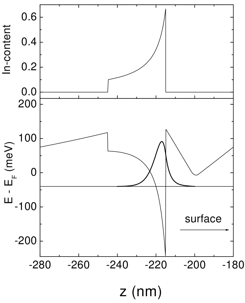
Figure 1: Calculated energy diagram and squared wave function for the investigated structure.

The samples were mesa etched into Hall bars with tree potential probes along each side and then an Ag or Al gate electrode was deposited by thermal evaporation onto the cap layer through a mask. The width of the bars and distance between the potential probes were 0.5 mm and 1 mm, respectively. Although varying the gate voltage $V_{g}$ we were able to change the density of electron gas in the QW from $4\times 10^{15}$ to $8.5\times 10^{15}$ m^-2, the most part of results presented here relate to $V_{g}=0$ (exception is Fig. 5). The parameters of electron gas for $V_{g}=0$ are the following: $n=8\times 10^{15}$ m^-2, $\sigma\simeq 3.1\times 10^{-3}$ $\Omega^{-1}\Box$ at $T=1.4$ K, the mean free path $l=370$ nm, the effective electron mass obtained from the Shubnikov-de Haas experiment is $(0.053\pm 0.005)m_{0}$, the diffusion coefficient $D$ is approximately equal to $0.09$ m²/s.

The transverse magnetoresistance was measured in perpendicular magnetic field up to 2 mT with step $0.01$ mT within the temperature range $0.45-5.0$ K. In order to apply tesla-scale in-plane magnetic field while sweeping subgauss control of perpendicular field, we mount the sample with 2D electrons aligned to the axis of primary solenoid (accurate to $\sim 1^{\circ}$) and use an independent split-coil solenoid to provide $B_{\perp}$ as well as to compensate for sample misalignment. The two calibrated Hall probes were used to measure $B_{\perp}$ and $B_{\parallel}$. Since antilocalization behavior of the magnetoresistance is observed at perpendicular field less than $0.2$ mT it is very important that the gradient of the perpendicular component of the tesla-scale in-plane magnetic field $B_{\perp}^{\parallel}$ was less than 0.01 mT/mm. To assure that this condition is fulfilled the magnetoresistance was measured simultaneously on two neighbor potential pairs placed along one side of the bar (see inset in Fig. 2).

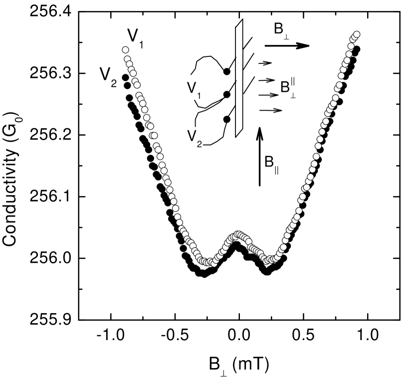
Figure 2: The conductivity as a function of perpendicular magnetic field measured at $B_{\parallel}=0.3$ T and $T=1.4$ K for two neighbor pairs of potential probes as shown in inset. Arrows in inset marked as $B_{\perp}^{\parallel}$ show perpendicular component of in-plane magnetic field which varies along the sample due to imperfection of magnet system.

The shift of these magnetoresistance curves relative to each other in $B_{\perp}$-direction is proportional to the gradient. To decrease the gradient along the structure there was needed to remove all, even slight, magnetic details and find an optimal position of the sample in primary solenoid. Fig. 2 shows that as a result of such procedures we have reduced the gradient of perpendicular component of in-plane magnetic field down to $1.6~{}10^{-4}B_{\parallel}/$mm.

III Magnetoresistance in a perpendicular field

Let us discuss the low-field magnetoresistance at zero in-plane field. The expression for the magnetoconductivity in a perpendicular field has the form

$$\sigma(B_{\perp})-\sigma(0)={G_{0}\over 2}\left[F_{t}\left(b_{\phi},b_{s}\right)-F_{s}\left(b_{\phi}\right)\right],$$ (1)

where $G_{0}=e^{2}/2\pi^{2}\hbar$, $b_{\phi}=B_{\phi}/B_{\perp}$, and $b_{s}=B_{s}/B_{\perp}$. The first term in Eq. (1) is the interference contribution of scattered electrons with the total momentum equal to one, i.e. being in the triplet state, and the second term is the singlet part. The latter depends only on one parameter $B_{\phi}=\hbar/4eD\tau_{\phi}$, where $\tau_{\phi}$ is the phase relaxation time. The triplet contribution depends not only on the dephasing rate but also on the spin relaxation time $\tau_{s}$ via the parameter $B_{s}=\hbar/4eD\tau_{s}$.

Spin relaxation in InGaAs QWs with low In content is caused by spin splitting of electron spectrum (the D’yakonov-Perel’ mechanism). The Hamiltonian of corresponding spin-orbit interaction is given by

$$H_{SO}(\bm{k})=\hbar{\bm{\sigma}}\cdot{\bm{\Omega}}({\bm{k}}),$$ (2)

where $\bm{\sigma}$ is the vector of Pauli matrices and the 2D vector in the plane of QW, $\bm{\Omega}$, is an odd function of ${\bm{k}}$. There are the Rashba ($\bm{\Omega}_{R}$) and Dresselhaus ($\bm{\Omega}_{D}$, $\bm{\Omega}_{3}$) contributions to $\bm{\Omega}$. The Rashba term for Fermi electrons has the form

$$\hbar\bm{\Omega}_{R}=\alpha k_{\rm F}(\sin{\varphi},-\cos{\varphi}),$$ (3)

where $\varphi$ is the angle between $\bm{k}$ and the [100] axis, $k_{\rm F}$ is the Fermi wavevector, and the constant $\alpha$ is given byalpha1 ; alpha2 ; alpha3

$$\alpha={P^{2}\over 3}\int dz\,\psi^{*}{d\over dz}\left[{1\over E_{\rm F}-E_{\Gamma_{7}}(z)}-{1\over E_{\rm F}-E_{\Gamma_{8}}(z)}\right]\psi.$$ (4)

Here, $\psi$ is the wave function of 2D electrons, $P$ is the Kane matrix element, $E_{\rm F}$ is the Fermi energy, and $E_{\Gamma_{7}}(z)$ and $E_{\Gamma_{8}}(z)$ are the band edge energies for $\Gamma_{7}$ and $\Gamma_{8}$ valence bands, respectively, at position $z$.

The Dresselhaus term $\bm{\Omega}_{D}$ also being the first Fourier-harmonic of $\varphi$, has the following form in [001]-grown QWs

$$\hbar\bm{\Omega}_{D}=\gamma k_{\rm F}\left(\langle k_{z}^{2}\rangle-{k_{\rm F}^{2}\over 4}\right)(\cos{\varphi},-\sin{\varphi}),$$ (5)

where $\gamma$ is the bulk constant of spin-orbit interaction, and $\langle k_{z}^{2}\rangle$ is the mean square of electron momentum in the growth direction

$$\langle k_{z}^{2}\rangle=\int dz\,\psi^{*}\left(-{d^{2}\over dz^{2}}\right)\psi.$$ (6)

The third harmonic of the Dresselhaus term, $\bm{\Omega}_{3}$, is given by

$$\hbar\bm{\Omega}_{3}=\gamma{k_{\rm F}^{3}\over 4}\>(\cos{3\varphi},-\sin{3\varphi}).$$ (7)

The theory of interference induced magnetoresistance in 2D systems with spin-orbit interaction Eq. (2) has been developed in Ref. ILP, . The authors derived an analytical expression for the magnetic field dependence of the conductivity when only $\Omega_{D}$ and $\Omega_{3}$ (or $\Omega_{R}$ and $\Omega_{3}$) contribute to the interference correction. Below we show that the magnetoresistance curves for the studied sample are well described with taking into account only $\Omega_{D}$. In this case, the spin relaxation time for the parameter $B_{s}$ is given by the expression

$${1\over\tau_{s}}=2\Omega_{D}^{2}\tau_{p},$$ (8)

where $\tau_{p}$ is the momentum scattering time. It is worth to mention that $\tau_{s}$ in the above expression coincides with the D’yakonov-Perel’ relaxation time for a spin lying in the QW plane.

The expressions for the functions $F_{s}$ and $F_{t}$ are derived in Ref. ILP, in a so-called diffusion approximation. It is valid for magnetic fields $B_{\perp}\ll B_{tr}$, where $B_{tr}=\hbar/4eD\tau_{p}$ is the “transport” field. A theory for high fields is developed in Ref. WAL_Yulik_PRL, accounting for the presence of all three terms in $\bm{\Omega}$. The obtained expressions, however, are valid for $B_{\perp}\gg B_{s}$. In our samples with moderate mobility, the transport field is strong enough ($B_{tr}=2.4$ T) so that the antilocalization minimum in magnetoconductivity takes place at $B_{\perp}\sim B_{s}<B_{tr}$. This allows us to extract the dephasing times $\tau_{s}$, $\tau_{\phi}$ from the low-field range where the diffusion approximation is valid.

Under these circumstances, the function $F_{s}(b_{\phi})$ is given by

$$F_{s}(b_{\phi})=\Psi(1/2+b_{\phi})-\ln{b_{\phi}},$$ (9)

where $\Psi$ is the digamma-function. The expression for $F_{t}(b_{\phi},b_{s})$ is as followsILP ; Lenya

$$F_{t}(b_{\phi},b_{s}) = \sum_{n=1}^{\infty}\left\{{3\over n}-{3a_{n}^{2}+2a_{n}b_{s}-1-2(2n+1)b_{s}\over(a_{n}+b_{s})a_{n-1}a_{n+1}-2b_{s}[(2n+1)a_{n}-1]}\right\}-{1\over a_{0}}-{2a_{0}+1+b_{s}\over a_{1}(a_{0}+b_{s})-2{b_{s}}}$$ (10)

$$- 2\ln{(b_{\phi}+b_{s})}-\ln{(b_{\phi}+2b_{s})}-3C-S(b_{\phi}/b_{s})$$

with $C\approx 0.57721$ as the Euler constant, $a_{n}=n+1/2+b_{\phi}+b_{s}$, and the $B_{\perp}$-independent function $S(b_{\phi}/b_{s})$ is given by

$$S(x)={8\over\sqrt{7+16x}}\left[\arctan{\left({\sqrt{7+16x}\over 1-2x}\right)}-\pi\Theta(1-2x)\right],$$ (11)

where $\Theta(y)$ is the Heaviside step function.

The experimental curves $\Delta\sigma(B_{\perp})=\rho_{xx}^{-1}(B_{\perp})-\rho_{xx}^{-1}(0)$ measured at $V_{g}=0$ for different temperatures and the fit by Eq. (1) with $\tau_{\phi}$ and $\tau_{s}$ as fitting parameters are presented in Fig. 3.

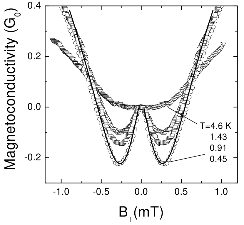
Figure 3: The low-field magnetoconductivity at different temperatures for $B_{\parallel}=0$ (symbols). Solid line is the best fit by Eq. (1) with the parameters $\tau_{\phi}=72$ ps and $\tau_{s}=8.8$ ps.

The fit was carried out within magnetic field range $0<B_{\perp}<0.3\,B_{tr}$. The temperature dependences of the phase and spin relaxation times found by this way are presented in Fig. 4.

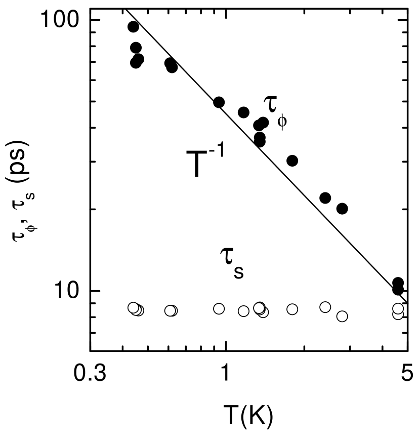
Figure 4: The temperature dependences of the phase and spin relaxation times for $V_{g}=0$ and $B_{\parallel}=0$.

It is evident that the behavior of $\tau_{\phi}$ is close to $T^{-1}$-law predicted theoretically, AA whereas $\tau_{s}$ is temperature independent that corresponds to the D’yakonov-Perel’ mechanism of spin relaxation in a degenerate electron gas.

The good agreement allows us to find the value of spin-orbit splitting $\hbar\Omega$. Such analysis has been carried out for wide range of electron density and final results are presented in Fig. 5.

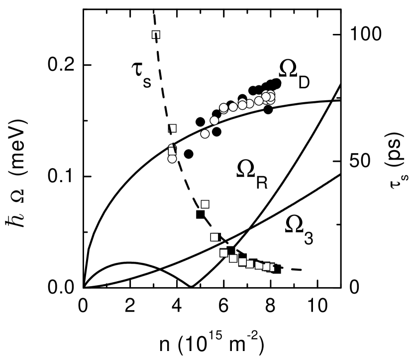
Figure 5: The values of $\hbar\Omega_{R}$, $\hbar\Omega_{D}$, $\hbar\Omega_{3}$ (circles) and $\tau_{s}$ (squares) as functions of electron density for the investigated structures. Open and solid symbols are the experimental data for $T=0.45$ K and $1.5$ K, respectively. The lines are the result of self-consistent calculationsOur1 in which we used $\gamma=18$ eV ų.

In the same figure, the electron density dependence is shown for all three terms $\Omega_{D}$, $\Omega_{R}$, and $\Omega_{3}$ found from self-consistent calculations for the studied structure by using Eqs. (3)-(7). One can see that the experimental data are close to the Dresselhaus term $\Omega_{D}$ which dominates both $\Omega_{3}$ and the Rashba term $\Omega_{R}$ within actual range of electron density.

IV Transverse magnetoresistance in the presence of in-plane magnetic field

Now let us discuss the effect of an in-plane magnetic field. The magnetoconductance versus perpendicular magnetic field measured for different $B_{\parallel}$ is presented in Fig. 6.

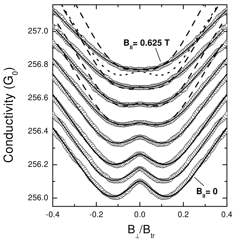
Figure 6: The conductivity as a function of $B_{\perp}$, measured at $T=1.4$ K for different in-plane magnetic fields $B_{\parallel}$: $0$, $0.075$, $0.125$, $0.225$, $0.325$, $0.425$, $0.525$ and $0.625$ T. The dashed curves are the best fit with only Zeeman contribution for some values of $B_{\parallel}$. Dotted curve illustrates the result of the fit with only Zeeman contribution carried out in the range of $B_{\perp}/B_{tr}$ from $0$ to $0.3$. The solid curves are the best fit when both roughness and Zeeman splitting are taken into account carried out with $B_{\phi}=0.0625$ mT and $B_{s}=0.28$ mT found at $B_{\parallel}=0$ and $\Delta_{s}$ and $\Delta_{r}$ presented in Fig. 7. For clarity, the plots are separated in vertical direction by the value of 0.1$G_{0}$.

It is seen that application of in-plane magnetic field decreases the depth of antilocalization minimum which disappears at $B\simeq(0.5-0.6)$ T.

The influence of in-plane magnetic field on the interference induced magnetoconductance is due to Zeeman splitting and interface microroughness. We start our consideration with Zeeman effect. The in-plane magnetic field couples the triplet and singlet states of interfering carriers. This makes Eq. (1) incorrect. However the applied magnetic fields are not too strong in our experiments: the condition

$$g\mu_{\rm B}B_{\parallel}<\hbar/\tau_{s}$$

is met up to the highest $B_{\parallel}=0.625$ T. Here $g$ is the in-plane electron $g$-factor and $\mu_{\rm B}$ is the Bohr magneton. In such low parallel field, dephasing of the triplet state is still determined by zero-field values of $\tau_{s}$ and $\tau_{\phi}$. The Zeeman interaction affects only the singlet contribution resulting in its additional depasing. Malsh1 ; Malsh2 The corresponding correction to $B_{\phi}$ in the second term of Eq. (1), $\Delta_{s}$, has the form

$$\Delta_{s}={\tau_{s}\over 4e\hbar D}\left(g\mu_{\rm B}B_{\parallel}\right)^{2}.$$ (12)

As a result, we get the expression for the interference induced transverse magnetoresistance in the presence of an in-plane magnetic field is given by

$$\sigma(B_{\perp},B_{\parallel})-\sigma(0,B_{\parallel})={G_{0}\over 2}\biggl{[}F_{t}\left(b_{\phi},b_{s}\right)-F_{s}\left(b^{\prime}_{\phi}\right)\biggr{]},$$ (13)

where

$$b^{\prime}_{\phi}={B_{\phi}+\Delta_{s}(B_{\parallel})\over B_{\perp}},$$

and the functions $F_{s}$, $F_{t}$ are given by Eqs. (8) and (10).

Results of the fit of experimental data by Eq. (13) with $\tau_{\phi}$, $\tau_{s}$ found at $B_{\parallel}=0$ and with $\Delta_{s}$ as fitting parameter are presented in Fig. 6 by dashed lines. As seen the range of $B_{\perp}$ in which a good fit can be achieved, narrows rapidly with increasing of $B_{\parallel}$. If the fitting range is kept constant, it is impossible to describe the transverse magnetoconductivity in the presence of in-plane magnetic field even qualitatively (dotted curve in Fig. 6). Thus, taking into account only Zeeman splitting does not give an agreement with experimental data. The reason for such discrepancy is the effect of microroughness.

Imperfections of the QW interfaces results in that an electron moving over QW shifts in the perpendicular direction also. This means that carriers in real 2D systems effectively feel random perpendicular magnetic field. This effect gives rise to the longitudinal magnetoresistance (considered in the next Section) and changes the transverse magnetoresistance in the presence of an in-plane field.

The effect of short-range roughness with $L\ll l$, where $L$ is the correlation length of the QW width fluctuations, on the shape of magnetoresistance is that application of an in-plane magnetic field also leads to additional dephasing. In areas with short-range fluctuations normal to the QW plane, carriers move transversely to the magnetic field $B_{\parallel}$. Their weak localization on these fluctuations is destroyed by $B_{\parallel}$. Quantitatively, in the presence of parallel magnetic field, the phase relaxation parameter $B_{\phi}$ acquires an addition Malsh2 ; Rough

$$B_{\phi}(B_{\parallel})=B_{\phi}(0)+\Delta_{r}(B_{\parallel}),$$ (14)

where

$$\Delta_{r}(B_{\parallel})\simeq{\sqrt{\pi}\over 2}{e\over\hbar}{d^{2}L\over l}B_{\parallel}^{2}.$$ (15)

Here, $d$ is the root-mean-square height of the fluctuations. Note, this effect manifests itself in the both singlet and triplet contributions in contrast to Zeeman splitting.

Thus, the final expression for $\sigma(B_{\perp},B_{\parallel})-\sigma(0,B_{\parallel})$ when both mechanisms are taken into account is

$$\sigma(B_{\perp},B_{\parallel})-\sigma(0,B_{\parallel})={G_{0}\over 2}\biggl{[}F_{t}\left(b_{\phi},b_{s}\right)-F_{s}\left(\widetilde{b}_{\phi}\right)\biggr{]},$$ (16)

where

$$\widetilde{b}_{\phi}={B_{\phi}+\Delta_{s}(B_{\parallel})+\Delta_{r}(B_{\parallel})\over B_{\perp}}$$

and

$$b_{\phi}={B_{\phi}+\Delta_{r}(B_{\parallel})\over B_{\perp}}.$$

The results of the fit by Eq. (16) with $\tau_{\phi}$, $\tau_{s}$ found at $B_{\parallel}=0$ and with $\Delta_{s}$ and $\Delta_{r}$ as fitting parameters are presented in Fig. 6 by solid lines. It is clearly seen that an excellent agreement occurs for all values of in-plane magnetic field.

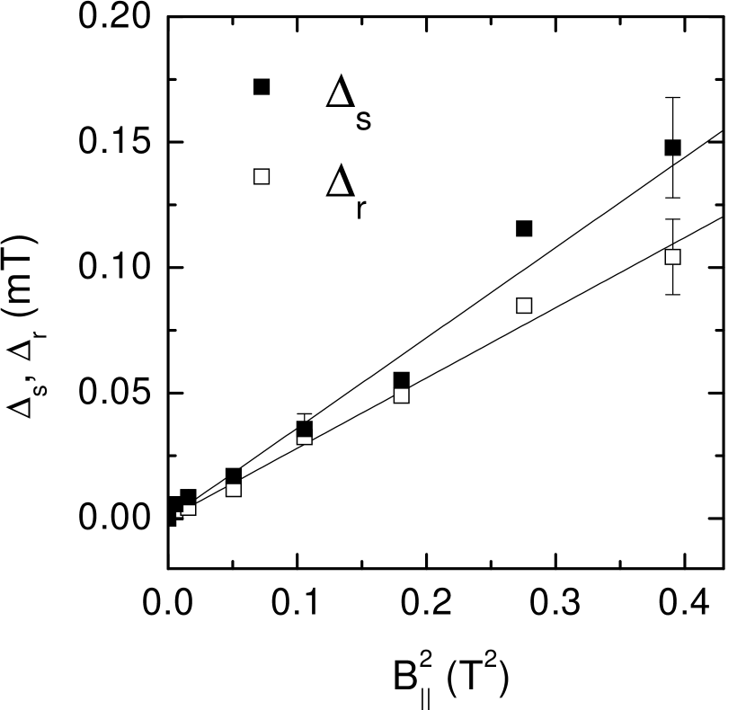
Figure 7: The value of the fitting parameters $\Delta_{s}$ and $\Delta_{r}$ corresponding to solid lines in Fig. 6 as a function of $B^{2}_{\parallel}$ (symbols). Upper line is Eq. (12) with $\tau_{s}=8.8$ ps, $D=0.09$ m²/s and $g=1.7$, lower one is Eq. (15) with $l=370$ nm and $d^{2}L=75$ nm³.

The used model predicts that the parameters $\Delta_{s}$ and $\Delta_{r}$ have to depend on $B_{\parallel}$ quadratically [see Eqs. (12) and (15), respectively]. Therefore in Fig. 7 we have presented the values of $\Delta_{s}$ and $\Delta_{r}$ as functions of $B_{\parallel}^{2}$. It is seen that these dependences are really close to quadratical ones within an experimental error. It allows us to determine the values of in-plane $g$-factor and parameter of roughness $d^{2}L$. We obtain $g=1.7\pm 0.3$ and $d^{2}L=(75\pm 15)$ nm³. This value of $g$-factor corresponds to that for bulk In_xGa_1-xAs with $x\simeq 0.35$, g-factor that in its turn agrees with average indium content within the QW (see Fig. 1). The value of $d^{2}L$ occurs several times larger than that obtained in Ref. ourProd, for analogous structures with In_0.2Ga_0.8As quantum well. We can explain this discrepancy by mechanical strain arising in heterostructures In_xGa_1-xAs/GaAs with sufficiently high indium content due to lattice mismatch.

Thus we successively described the anomalous magnetoresistance in a tilted field. The effects of the in-plane field component are shown to be important at $B_{\parallel}\sim 1/(g\mu_{\rm B}\sqrt{\tau_{s}\tau_{\phi}})\gg B_{\perp}$. This explains the observed resistance independence of a weak in-plane field $B_{\parallel}\sim B_{\perp}$.Stud

V Longitudinal magnetoresistance

Let turn now to the effects of pure in-plane field. Longitudinal magnetoresistance measured at T=1.4 K is shown by points in Fig. 8. As mentioned above the in-plane magnetic field does not destroy the electron interference of absolutely flat 2D gas of spinless particle and does not result in longitudinal magnetoresistance. However, in real systems this effect should be evident due to roughness of interface. Its magnitude can be easily estimated asRough

$$\sigma(B_{\parallel})-\sigma(0)=G_{0}\ln\left[1+{\Delta_{r}(B_{\parallel})\over B_{\phi}}\right].$$

Using $B_{\phi}=0.06$ mT and $\Delta_{r}(B_{\parallel})$ presented in Fig. 7 we obtain that the conductivity raising at $B_{\parallel}=0.6$ T has to be about $1\,G_{0}$ — see the dotted line in Fig. 8. In contrast to that, the measured longitudinal magnetoconductance does not exhibit strong $B_{\parallel}$-dependence. This points to importance of spin effects in weak localization for our structure once again.

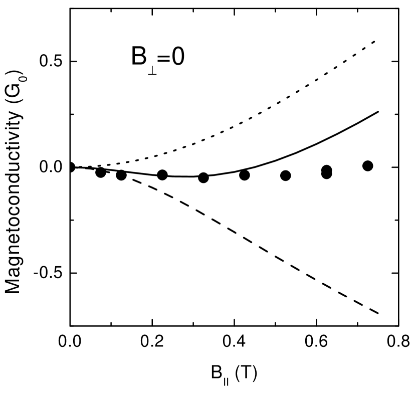
Figure 8: The longitudinal magnetoconductivity for $T=1.4$ K (symbols). Solid line is Eq. (17) with $B_{\phi}=0.0625$ mT, $B_{s}=0.28$ mT, and $\Delta_{r}(B_{\parallel})$ and $\Delta_{s}(B_{\parallel})$ shown in Fig. 7 by solid lines. Dotted and dashed lines are calculation results when only roughness ($\Delta_{s}=0$) or Zeeman effect ($\Delta_{r}=0$) is taken into account, respectively.

The expression for longitudinal magnetoresistance in the presence of both roughness and Zeeman splitting can be obtained from Eq. (16) in the limit $B_{\perp}\to 0$. As a result we have explicitly

$$\sigma(B_{\parallel})-\sigma(0)={G_{0}\over 2}\Biggl{[}2\ln\left({B_{\phi}+B_{s}+\Delta_{r}\over B_{\phi}+B_{s}}\right)$$ (17)

$$+ \ln\left({B_{\phi}+2B_{s}+\Delta_{r}\over B_{\phi}+2B_{s}}\right)-\ln\left({B_{\phi}+\Delta_{r}+\Delta_{s}\over B_{\phi}}\right)\Biggr{]}$$

$$+ S(B_{\phi}/B_{s}+\Delta_{r}/B_{s})-S(B_{\phi}/B_{s}),$$

where the function $S(x)$ is given by Eq. (11). Solid line in Fig. 8 is the longitudinal magnetoresistance calculated according to Eq. (17) with $\Delta_{r}(B_{\parallel})$ and $\Delta_{s}(B_{\parallel})$ parabolic dependences shown in Fig. 7 by solid lines. One can see satisfactory agreement between experimental and calculated results. The dotted and dashed line illustrate separate contributions of microroughness and Zeeman effect in longitudinal magnetoconductance. One can see that they are of opposite sign and compensate each other to a large extent. It should be noted that such a compensation is not universal. The sign and relative contribution of the considered effects is determined by the parameters of concrete system entering into Eq. (17).

VI Conclusion

In conclusion, we have measured the anomalous magnetoresistance in a field perpendicular, tilted and parallel to the QW plane. Weak-antilocalization theory describes the data very well allowing to obtain the spin and phase relaxation times. Our study demonstrates that spin dephasing leading to weak antilocalization is due to the Dresselhaus spin-orbit interaction which dominates the Rashba term in our structures.

Application of an in-plane magnetic field is shown to destroy weak antilocalization due to competition of Zeeman and microroughness effects. From the analysis of longitudinal magnetoconductivity we extracted the characteristics of short-range interface imperfections and the value of the in-plane electron $g$-factor.

References

- (1) Semiconductor Spintronics and Quantum Computation, eds. D.D. Awschalom, D.Loss, and N. Samarth (Springer, Berlin, 2002).
- (2) H.L. Stormer, Z. Schlesinger, A. Chang, D.C. Tsui, A.C. Gossard, and W. Wiegmann, Phys. Rev. Lett. 51, 126 (1983).
- (3) D. Stein, K. von Klitzing, and G. Weimann, Phys. Rev. Lett. 51, 130 (1983).
- (4) Yu.L. Bychkov and É.I. Rashba, Pis’ma Zh. Eksp. Teor. Fiz. 39, 66 (1984) [JETP Lett. 39, 78 (1984)]; J. Phys. C 17, 6039 (1984).
- (5) B.L. Altshuler and A.G. Aronov, in Electron-electron interactions in disordered systems, edited by A.L. Efros and M. Pollak, (Elsevier, Amsterdam, 1985).
- (6) S. Hikami, A. Larkin, and Y. Nagaoka, Progr. Theor. Phys. 63, 707 (1980).
- (7) G. Bergmann, Phys. Rep. 107, 1 (1984).
- (8) P.D. Dresselhaus, C.M.M. Papavassiliou, R.G. Wheeler and R.N. Sacks, Phys. Rev. Lett. 68, 106 (1992).
- (9) G.L. Chen, J. Han, T.T. Huang, S. Datta, and D.B. Janes, Phys. Rev. B 47, 4084 (1993).
- (10) S.V. Iordanskii, Yu.B. Lyanda-Geller and G.E. Pikus, Pis’ma Zh. Eksp. Teor. Fiz. 60, 199 (1994) [JETP Lett. 60, 206 (1994)].
- (11) F.G. Pikus and G.E. Pikus, Phys. Rev. B 51, 16928 (1995).
- (12) W. Knap, C. Skierbiszewski, A. Zduniak, E. Litvin-Staszevska, D. Bertho, F. Kobbi, J.L. Robert, G.E. Pikus, F.G. Pikus, S.V. Iordanskii, V. Moser, K. Zekentes, and Yu.B. Lyanda-Geller, Phys. Rev. B53, 3912 (1996).
- (13) T. Hassenkam, S. Pedersen, K. Baklanov, A. Kristensen, C.B. Sorensen, P.E. Lindelof, F. G. Pikus, and G.E. Pikus, Phys. Rev. B 55, 9298 (1997).
- (14) T. Koga, J. Nitta, T. Akazaki, and H. Takayanagi, Phys. Rev. Lett. 89, 46801 (2002).
- (15) A.G. Mal’shukov, K.A. Chao, and M. Willander, Phys. Rev. B 56, 6436 (1997).
- (16) A.G. Mal’shukov, V.A. Froltsov, and K.A. Chao, Phys. Rev. B 59, 5702 (1999).
- (17) H. Mathur and H.U. Baranger, Phys. Rev. B 64, 235325 (2001).
- (18) D.M. Zumbühl, J.B. Miller, C.M. Marcus, K. Campman, and A.C. Gossard, Phys. Rev. Lett. 89, 276803 (2002).
- (19) The energy spectrum and electron charge distribution in the growth direction have been obtained as a result of simultaneous solution of the Schrödinger and Poisson equations.
- (20) J.B. Miller, D.M. Zumbühl, C.M. Marcus, Y.B. Lyanda-Geller, D. Goldhaber-Gordon, K. Campman, and A.C. Gossard, Phys. Rev. Lett. 90, 076807 (2003).
- (21) L.G. Gerchikov and A.V. Subashiev, Fiz. Techn. Poluprov. 26, 131 (1992) [Sov. Phys. Semicond. 26, 73 (1992)].
- (22) E. A. de Andrada e Silva, G.C. La Rocca, and F. Bassani, Phys. Rev. B50, 8523 (1994).
- (23) P. Pfeffer, Phys. Rev. B59, 5312 (1999).
- (24) G.M. Minkov, A.V. Germanenko, O.E. Rut, A.A. Sherstobitov, B.N. Zvonkov, cond-mat/0311238, to appear in Int. J. Nanoscience.
- (25) In Ref. ILP, the expression for the weak-localization contribution to the conductivity is given. We have calculated the limit and arrived at the Eq. (1).
- (26) C. Hermann and C. Weisbuch, Phys. Rev. B 15, 823 (1977).
- (27) G.M. Minkov, O.E. Rut, A.V. Germanenko, A.A. Sherstobitov, B.N. Zvonkov, and D.O. Filatov, cond-mat/0311124.
- (28) S.A. Studenikin, P.T. Coleridge, N. Ahmed, P.J. Poole, and A. Sachrajda Phys. Rev. B 68, 035317 (2003).