Zero Temperature Glass Transition in the Two-Dimensional Gauge Glass Model

Abstract

We investigate dynamic scaling properties of the two-dimensional gauge glass model for the vortex glass phase in superconductors with quenched disorder. From extensive Monte Carlo simulations we obtain static and dynamic finite size scaling behavior, where the static simulations use a temperature exchange method to ensure convergence at low temperatures. Both static and dynamic scaling of Monte Carlo data is consistent with a glass transition at zero temperature, with correlation length exponent given by $1/\nu=0.36\pm 0.03$. We study a dynamic correlation function for the superconducting order parameter, as well as the phase slip resistance. From the scaling of these two functions, we find evidence for two distinct diverging correlation times at the zero temperature glass transition. The longer of these time scales is associated with phase slip fluctuations across the system that lead to finite resistance at any finite temperature. The shorter time scale can be described by the form $\tau\sim\xi^{z}$, with a dynamic exponent $z=2.7\pm 0.2$, and corresponds to local phase fluctuations.

I Introduction

Despite intense studies of the superconducting glass transition in vortex systems, the precise nature of the transition remains controversial. The presence of quenched disorder in a strongly type II superconductor in an applied magnetic field may create a superconducting vortex glass phase with zero linear resistance, where the vortices are localized in random positions given by the disorder and interactions Fisher (1989). Considerable theoretical and simulation efforts have been focused on whether a superconducting glass state exists at finite temperature, or alternatively, only at zero temperature. In particular the situation in two dimensions still remains debated. In this paper we present results from Monte Carlo simulation and finite size scaling analysis for the glass transition in two dimensions. We focus mainly on the dynamic scaling properties, which have not been studied in detail before, using a dynamic scaling ansatz for a zero temperature transition. From our static and dynamic scaling analysis, we find evidence for a zero temperature glass transition, and present various predictions for the physical properties at the transitions.

The gauge glass (GG) model is an XY model with a random quenched vector potential on the links of the lattice; see Eq. (1) below. The GG model contains important aspects of order parameter symmetry, interactions, and quenched disorder, and has been frequently studied as a model for a vortex glass transition. In a real glass, the system may fall out of equilibrium at the transition, but here we focus on the equilibrium critical behavior of the model. This enables the study of universal scaling laws at the transition, that depend only on the universality class. It has not been settled if the GG model represents the correct universality class of the vortex glass transition, and it is thus motivated to obtain the precise critical behavior of the GG model. The GG model is not realistic in a few important aspects: disorder is included only in terms of a random vector potential, instead of a random pinning energy for the vortex cores, and it has zero applied magnetic field. Alternatively, a suitable modification of the GG model as a model for the elastic energy of a dislocated vortex lattice is discussed in Ref. Lidmar, 2003. Another worry is the use of a classical model for a zero temperature transition, where quantum effects may be important. However, since vortices localize in the glass phase, their quantum fluctuations are small and can be neglected, and a classical treatment is a reasonable starting point, also at $T=0$. This neglects the possibility of quantum tunneling of vortices, which may actually be important.

Considerable simulation efforts have been invested in trying to locate the lower critical dimension $d_{c}$ of the vortex glass transition, i.e., the limiting dimensionality such that a glass phase exists at finite temperature only for $d>d_{c}$. In the 3D case, several simulations Reger et al. (1991); Olson and Young (2000); Katzgraber and Young (2002) show that a vortex glass phase does exist at finite temperatures in the absence of magnetic screening. In 2D the situation is less clear. It has been shown rigorously that there can be no vortex-glass order in 2D for $T>0$ Nishimori (1994). For a finite screening length it is expected that no glass phase can exist at $T>0$ Bokil and Young (1995). Akino and Kosterlitz computed the domain wall stiffness exponent $\theta$ at zero temperature, and obtained a negative value, $\theta=-0.36$, indicating that $T_{c}=0$ Akino and Kosterlitz (2002). Holme and Olsson computed the energy barrier for vortex motion across the system and argue that $T_{c}>0$ Holme and Olsson (2002). Katzgraber and Young recently obtained $T_{c}=0$ and $\theta=-1/\nu=-0.39\pm 0.03$ from finite temperature simulations Katzgraber and Young (2002); Katzgraber (2003). In contrast, several other studies of static quantities obtained $T_{c}\approx 0.2$ Holme et al. (2003); Choi and Park (1999). Dynamic scaling in the 2D GG model has been studied in several papers Li (1992); Kim (2000); Choi and Park (1999); Hyman et al. (1995); Wengel and Young (1996); Katzgraber and Campbell (2004), with conflicting results. It is important to consider dynamic scaling in order to obtain information about physically measurable quantities like the resistance. Previous studies of zero temperature scaling of dynamic properties considered nonlinear $I-V$ characteristics Hyman et al. (1995), and in addition the linear resistance was found to be roughly consistent with a simple Arrhenius form Hyman et al. (1995); Wengel and Young (1996), $R\sim e^{-K/T}$, but no further support for zero temperature dynamic scaling has been obtained. In contrast, Refs. Li, 1992; Kim, 2000; Choi and Park, 1999 obtained $T_{c}>0$ from vortex dynamics simulations. Hence the behavior of the GG model remain controversial, in particular for the dynamic properties.

In this paper we study critical scaling properties at the glass transition for both dynamic and static quantities, assuming a zero temperature transition. Our simulations are motivated in part by new methods that have recently been developed. At low temperature the correlation times in the simulation grow very long and efficient convergence acceleration methods become highly desirable. The temperature exchange method Hukushima and Nemoto (1996); Marinari (1998) has proven very useful for such problems, where configurations are exchanged between different temperatures, in order to avoid getting stuck in metastable states. This considerably speeds up the convergence of the simulation, and thereby enables simulation at larger system sizes and lower temperatures. Our scaling results for static quantities are in good agreement with some of the previous results in the literature for the correlation length exponent and the domain wall energy exponent $\theta$ Hyman et al. (1995); Wengel and Young (1996); Katzgraber and Young (2002); Katzgraber (2003); Akino and Kosterlitz (2002). For our dynamics simulations we also get valuable input from the exchange method, even though exchange is not directly applicable for dynamics, by using typical equilibrium configurations from the exchange runs as input to the dynamics runs. This considerably extends the regime of temperatures and system sizes accessible for the dynamics simulation. The main new results of our work are for the dynamic finite size scaling analysis of the linear resistance and of the dynamic correlation function for the order parameter at the zero temperature glass transition. We obtain correlation times from finite size scaling of our dynamic MC data that show novel behavior. We find evidence for two distinct diverging correlation times, one associated with phase slip fluctuations, and the other associated with local phase fluctuations that are independent of the phase slip processes.

The organization of the paper is as follows: In Sec. II we introduce the GG model and describe our simulation methods. In Sec. III we discuss the quantities calculated in the simulation and the finite size scaling methods. In Sec. IV the static results are presented, and Sec. V contains the results for the dynamic quantities. Section VI contains discussion and conclusions.

II Model and Monte Carlo simulation details

The gauge glass (GG) model Shih et al. (1984); Huse and Seung (1990); Fisher et al. (1991) is defined by the Hamiltonian

$$H=-\sum_{{\langle}i,j{\rangle}}\cos(\theta_{i}-\theta_{j}-A_{ij})$$ (1)

where $\theta_{i}$ is the phase of the superconducting order parameter on site $i$ of a square lattice, and $\sum_{{\langle}i,j{\rangle}}$ denotes summation over all nearest-neighbor pairs in the lattice. The vector potential enters through $A_{ij}=\frac{2\pi}{\phi_{0}}\int_{i}^{j}d{\bf r}\cdot{\bf A}$, which is a quenched random variable on each link in the lattice, with a uniform probability distribution in $[0,2\pi)$, corresponding to fixed random magnetic induction ${\bf B}=\nabla\times{\bf A}$ through the plaquettes of the lattice. The partition function is $Z=\left(\prod_{j}\int_{0}^{2\pi}d\theta_{j}\right)\exp(-H/T)$, where $T$ is the temperature. The simulation uses square lattices of size $L\times L$ with periodic boundary conditions (PBC) in both the $x$ and $y$-directions.

We also consider the GG model with different boundary conditions, where the system repeats periodically, but with fluctuating phase twist variables $\Delta_{x},\Delta_{y}$ added to the respective phase differences across the boundary of the system. This allows for phase twist fluctuations across the system, and enables calculation of the resistance of the model, as is discussed below. In this case the Hamiltonian is

$$H=-\sum_{{\langle}i,j{\rangle}}\cos(\theta_{i}-\theta_{j}-A_{ij}-\delta_{x_{i},L}\Delta_{x}-\delta_{y_{i},L}\Delta_{y})$$ (2)

where $\Delta_{x},\Delta_{y}$ are integrated over $(-\infty,\infty)$ in the partition function. In a static simulation, the partition function is invariant if the the phase twist at the boundary is spread out in the bulk as a constant extra phase difference $\Delta/L$ on each link. However, dynamically these both prescriptions are different. We define the phase twist fluctuations located at the boundary in order to maintain local dynamics.

In the Monte Carlo simulations the trial moves are attempts to assign the phase, at a randomly chosen site, a random value from a uniform distribution in $[0,2\pi)$. The moves are accepted with probability $1/(1+\exp\Delta E/T)$, where $\Delta E$ is the energy difference for the trial move. One sweep is defined as on average one attempt to update each phase. In the simulations of static quantities we use a temperature exchange method Hukushima and Nemoto (1996); Marinari (1998), that considerably enhances the convergence of the simulations at low temperature and big system sizes. We use ten sweeps of local MC moves, followed by one exchange sweep. In the exchange sweep the trial moves are attempts to exchange configurations between neighboring temperatures, where up to 39 closely spaced temperatures, with $T_{n}=T_{n-1}(1-1/L)$, are simulated in parallel, sharing the same disorder realization. The exchange moves are accepted with probability $\exp[-(\beta_{n}-\beta_{n+1})(E_{n+1}-E_{n})]$, where $\beta=1/T$. To reach equilibrium we discard up to $6\cdot 10^{4}$ MC sweeps, followed by equally many sweeps where data is collected. The results are averaged over up to $10^{4}$ realizations of the random vector potential $A_{ij}$. To avoid systematic errors in the calculation of squares of expectation values, two replicas of the system with the same disorder are used. We use various tests to verify that sufficient equilibration is achieved, which will be presented in the results section below. In this paper we denote thermal averages by ${\langle}\cdots{\rangle}$, and disorder averages by $[\cdots]$.

In the simulation of dynamic quantities the exchange MC method does not apply directly, since we must use a method that respects the local nature of the dynamics of the system. Instead we use the usual Monte Carlo scheme with local updates of the phase. However, also for the dynamics runs we take advantage of the exchange algorithm in two ways. First, we use equilibrium configurations from an exchange run as initial configurations for the dynamics runs. Second, during the dynamics simulation we also recalculate the static quantities, and compare to the same quantities from the exchange runs. This gives an additional test of convergence for the dynamics simulation. We define one time step to be one MC sweep through the system with local updates. In the simulation with fluctuating twists, one time step corresponds to one sweep with local phase updates, followed by one update of $\Delta_{x}$ and of $\Delta_{y}$. The phase twist updates are attempts to add a uniformly distributed random number in $(-\pi,\pi)$. As initial configurations in the dynamics runs, we use configurations generated in an exchange run, followed by up to $4\cdot 10^{5}$ sweeps of local MC moves where data is taken. Occasional runs with even more sweeps were also used to test convergence. Disorder averages are formed over up to $10^{4}$ realizations of the disorder. We stress that there are many dynamic universality classes, and here we only consider that of local relaxation of the phase, which has proven useful in previous studies of the superconducting phase transition Hyman et al. (1995); Lidmar et al. (1998).

III Calculated quantities and finite size scaling relations

The basic quantity in our analysis of thermodynamic properties of the glass transition is the root mean square (RMS) current Reger et al. (1991); Olson and Young (2000). The current in the $x$-direction is defined as the derivative of the free energy $F$ with respect to a phase twist $\Delta_{x}$ on the boundary in the $x$-direction, for $\Delta_{x}=0$:

$$I=\left.\frac{\partial F}{\partial\Delta_{x}}\right|_{\Delta_{x}=0}=\frac{1}{L}\sum_{j}{\langle}\sin(\theta_{j+\hat{x}}-\theta_{j}-A_{j,j+\hat{x}}){\rangle}$$ (3)

where $j+\hat{x}$ denotes the nearest neighbor (NN) site next to $j$ in the $x$-direction. Here the phase twist $\Delta_{x}$ at the boundary has been absorbed into the bulk by adding a uniform phase twist $A=\Delta_{x}/L$ on each link in the $x$-direction, which gives the $1/L$ factor in the last equation. The RMS current is defined as

$$I_{\rm rms}=[I^{a}I^{b}]^{1/2}$$ (4)

where $a,b$ denote two replicas of the system sharing identical disorder.

In order to use the scaling properties of MC data to discriminate between the possibilities that $T_{c}=0$ and $T_{c}>0$, we must formulate suitable scaling assumptions for each case Hyman et al. (1995); Katzgraber and Young (2002). At the glass transition the correlation length is assumed to diverge as $\xi\sim|T-T_{c}|^{-\nu}$ if $T_{c}>0$, and as $\xi\sim T^{-\nu}$ if $T_{c}=0$. In the case $T_{c}>0$, we assume that close to $T_{c}$ the RMS current obeys the finite size scaling relation Olson and Young (2000)

$$I_{\rm rms}(T,L)=\tilde{I}(L^{1/\nu}(T-T_{c}))$$ (5)

where $\tilde{I}$ is a universal scaling function. This scaling form implies that the RMS current is independent of system size $L$ at $T=T_{c}$, which gives a convenient criterion for locating $T_{c}$. In contrast, if $T_{c}=0$, the scaling relation becomes modified, since for $T_{c}=0$ we have $\xi\sim T^{-\nu}=\beta^{\nu}$, and hence $\beta\sim\xi^{1/\nu}$, which must be included in the scaling relation. This gives $\beta I=\partial\beta F/\partial\Delta\sim\xi^{0}$. The scaling ansatz for the RMS current valid for the case $T_{c}=0$ becomes

$$I_{\rm rms}(T,L)=L^{-1/\nu}\tilde{I}(L^{1/\nu}T)$$ (6)

Below we will compare both these scaling forms to our data, and find that the scaling form with $T_{c}>0$ is not fulfilled by our MC data, while the scaling form with $T_{c}=0$ works well.

Next we discuss the quantities that we calculate in the dynamic simulation, and their respective scaling relations. The aim of our analysis is to obtain scaling relations from a dynamic scaling ansatz that assumes $T_{c}=0$, and here we will only formulate the scaling relations for this case. The scaling relations will first be formulated in terms of the correlation time, $\tau$, whose scaling will in turn be discussed below.

The resistance can be calculated by using fluctuating twist boundary conditions instead of PBC. It is obtained from the Kubo formula for the voltage-voltage correlation function. We define a time dependent resistance function as

$$R(t,T,L)=\frac{1}{2T}\sum_{t^{\prime}=-t}^{t}\Delta t^{\prime}\left[{\langle}V(t^{\prime})V(0){\rangle}\right]$$ (7)

where the voltage at MC timestep $t$ is given by the Josephson relation $V(t)=\frac{\hbar}{2e}\frac{d\Delta_{x}}{dt}$ (we henceforth assume units such that $\hbar/2e=1$). Here $d\Delta_{x}/dt$ is the rate of change of the phase shift across the system in the $x$-direction, which gives the resistance in the $x$-direction. The usual Kubo formula Young (1994) for the resistance is obtained from this function in the limit when the summation over MC timesteps $t\to\infty$. In practice this limit means that the summation time has to be long enough that the resistance is independent of $t$. However, since this time is going to be very long in the simulation, it is quite useful to consider $R$ as a function of $t$ and study the scaling properties as function of $t$. Since the voltage scales as $V\sim 1/\tau$, we make the finite size scaling ansatz

$$R(t,T,L)=\frac{1}{\tau T}\tilde{R}(L^{1/\nu}T,t/\tau)$$ (8)

where $\tilde{R}$ is a scaling function.

Another useful quantity is the dynamic correlation function for the real part of the superconducting order parameter, $\Psi^{\prime}=\sum_{j}\cos\theta_{j}$, which is gauge dependent and hence not directly observable in a superconductor, but gives a convenient measure of the dynamic correlations of the local order in the system. We define the time dependent summed autocorrelation function

$$G(t,T,L)=\sum_{t^{\prime}=-t}^{t}\Delta t^{\prime}\left[\frac{{\langle}\Psi^{\prime}(t^{\prime})\Psi^{\prime}(0){\rangle}}{{\langle}\Psi^{\prime 2}{\rangle}}\right]$$ (9)

For $t\to\infty$, $G$ measures the correlation time $\tau$ of the fluctuations in $\Psi^{\prime}$, and we have

$$G(t,T,L)=\tau\tilde{G}(L^{1/\nu}T,t/\tau)$$ (10)

Note that all the (unknown) dynamic scaling functions contain two arguments, which complicates their analysis. We will make use of two possible ways to obtain a function of one variable only, and this function can then be conveniently analyzed. One way is to obtain data for $t\gg\tau$, and the second way is to fix the first argument to a constant value by using different temperatures for each system size so that $L^{1/\nu}T=const$ Hyman et al. (1995), which then permits scaling analysis of the entire $t/\tau$ dependence.

In order to quantitatively fit the dynamic scaling formulas to MC data, we need an ansatz for the form of $\tau$. This is related to the divergence of the free energy barriers at the glass transition. The thermodynamic free energy barrier exponent $\theta$ is defined from the interfacial free energy RMS difference, $U_{L}$, for changing the boundary condition in one direction from PBC to anti-PBC. For a system of size $L$ we have $U_{L}=KL^{\theta}$, where $K$ is a constant. Now, a change in free energy from a change in the boundary conditions must scale in the same way as the current in Eqs. (3) and (6), which gives $\theta=-1/\nu$. Thus $\theta$ can be obtained from analysis of $I$ at finite temperatures.

A dynamic barrier exponent $\psi$ can be defined by $V_{L}=KL^{\psi}$, which is the free energy cost to move a vortex a distance $L$ using only local moves. In general $V_{L}$ and $U_{L}$ do not need to coincide, and the dynamic barrier for vortex motion across the system can be very big. We assume that the correlation time scales in an activated form given by

$$\tau\sim\exp(V_{L}/T)\sim\exp(C/T^{1+\nu\psi})$$ (11)

where $C$ is a constant. If $\psi=0$ this reduces to a simple Arrhenius form, $\tau\sim\exp C/T$. We also consider a few other possibilities. The usual finite temperature form of the critical slowing down is $\tau\sim L^{z}$. Another possible form is a logarithmic barrier, $\tau\sim\exp K(\ln L)/T$.

IV Results for static quantities

We first study the approach to equilibration of the exchange MC simulation. This is necessary in order to avoid systematic errors due to insufficient equilibration. We consider the RMS current, $I_{\rm rms}$, defined in Eq. (4). Figure 1 shows some of our data for the RMS current as a function of simulation warmup time. The data points in the figure are calculated by first discarding $t$ MC sweeps, and then forming averages over equally many sweeps. In Fig. 1 we see that the equilibration time, where the curves become independent of $t$, becomes very long already for moderate system sizes $L$, despite the considerable convergence speed-up due to the exchange method.

Figure 1: Test of equilibration of MC data for the RMS current at $T=0.1$. Here $t$ sweeps are taken without any measurements, followed by another $t$ sweeps where data is collected. The saturation time in the plot gives an estimate of the necessary equilibration times for the different system sizes.

Next we consider finite size scaling properties of the RMS current. Figure 2 shows MC data for the RMS current vs. temperature. According to Eq. (5) data curves for $I_{\rm rms}$ should become system size independent and thus intersect at $T=T_{c}$, if $T_{c}>0$. The absence of any such intersection in the figure indicates that $T_{c}$ is much smaller than the temperatures where we have data, i.e., $T_{c}\ll 0.1$. Henceforth we will therefore assume that $T_{c}=0$.

Figure 2: MC data for the RMS current vs. temperature for different system sizes $L$. Finite size scaling arguments valid for $T_{c}>0$ (see text) show that data curves for different system sizes become independent of $L$ at $T=T_{c}$, and hence intersect. The absence of any intersection in the plot implies that $T_{c}\ll 0.1$. The data points connected by lines are produced by the temperature exchange method. The circles mark data points obtained without the exchange method, to allow calculation of dynamic quantities, and are in good agreement with the data points obtained from the exchange method, indicating that ensemble averages and dynamic averages tend to coincide.

To scale MC data for $I_{\rm rms}$ assuming that $T_{c}=0$, Eq. (6) shows that a plot of $L^{1/\nu}I_{\rm rms}$ vs. $L^{1/\nu}T$ for different $T,L$ should collapse onto a system size independent curve, for the correct value of $1/\nu$. Scaling plots are shown in Fig. 3 for the choices (a) $1/\nu=0.39$ and (b) $1/\nu=0.36$. In (a) we see that $1/\nu=0.39$ gives the best overall data collapse, but the fit is somewhat poor for the smallest values of $L^{1/\nu}T$, which for $T_{c}=0$ is expected to be the most significant part of the data collapse. We therefore drop data points for large $L^{1/\nu}T$ and only fit the value of $\nu$ to the data points with smallest $L^{1/\nu}T$. Fitting the data points at the two lowest temperatures for sizes $L=10,12,16$ to a straight line, and minimizing the RMS fit error, gives $\nu=0.36\pm 0.03$. The error bar is obtained by the bootstrap method Newman and Barkema (1999). The resulting data collapse is shown in Fig. 3 (b), and we see that, for small $L^{1/\nu}T$, a better fit is obtained than in (a). The estimate $\nu=0.36\pm 0.03$ is insensitive within the error bar to varying the precise details of the fit, such as including the three lowest temperatures for each $L$.

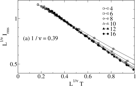
Figure 3: Finite size scaling plot of the MC data in Fig. 2 using Eq. (6) with $T_{c}=0$. In (a) $1/\nu=0.39$, which gives a data collapse except for the lowest temperatures and smallest system sizes. In (b) $1/\nu=0.36$, which gives a better data collapse at the smallest temperatures.

V Results for dynamic quantities

The dynamics simulations contain only local MC moves, and the averages computed in the dynamics runs correspond to time integration of the observables. The statics simulation contains both local MC moves and nonlocal temperature exchange moves that take big steps in configuration space, which corresponds to ensemble averaging. If ergodicity is broken these different averages may disagree Holme and Olsson (2002). To investigate this issue we plot the RMS current calculated in a dynamics run in Fig. 2, together with the corresponding result from the static simulation. The figure shows that the results from static and dynamic runs coincide within error bars.

We will make use of the following input from the statics simulations. The static scaling results gives the value of the correlation length exponent, which is needed also in the dynamic scaling analysis. We will assume the value $1/\nu=0.39$, but make occasional comparison with the corresponding results for $1/\nu=0.36$. Furthermore, the static scaling results also give an indication of the range of system sizes and temperatures where we can expect dynamic scaling of the data to hold. From Fig. 3 we estimate that dynamic scaling can be expected when $L^{1/\nu}T$ is smaller than about 0.8.

We expect that the longest emergent time scale comes from phase slip events corresponding to vortex motion across the sample. An illustration of these long correlation times is seen in Fig. 4, which shows phase slip events in a dynamic simulation where fluctuations in the boundary conditions are included, for a few different realizations of the quenched disorder. Phase slip events are often as far as about $10^{5}$ sweeps apart.

Figure 4: Examples from our simulation of the time evolution of MC data for the phase twist variable for a few different disorder realizations. The characteristic time scale for big fluctuations in the twist variable can be $>10^{5}$ sweeps. We identify such fluctuations as phase slips corresponding to vortex motion across the sample.

Figure 5 shows the time dependent resistance function given by Eq. (7) for $L^{0.39}T=0.8$. The data curves show unexpectedly complicated behavior, with a power-law regime at short times, and a time-independent limit at long times, with various crossover times in between. We will now analyze the scaling behavior of these different time scales.

Figure 5: MC data for the resistance function $R(t,T,L)$ vs. time $t$ for different system sizes for $A=L^{1/0.39}T=0.8$. The resistance curves have different characteristic regimes, one for $t>\tau$ where $R$ becomes independent of $t$, and one power-law regime for shorter times.

We first consider the long time limit, $t\gg\tau$, of the data curves in Fig. 5, which gives the resistance $R$. According to Eq. (8), the correct value of $\tau$ for each system size and temperature, such that $L^{1/\nu}T=A$ is a constant, should make data curves for $RT\tau$ plotted vs. $t/\tau$ collapse onto a common curve for $t\gg\tau$. Thus we adjust $\tau$ for each data curve to the value that gives the best collapse. The result is shown in Fig. 6. We obtain a data collapse to a common curve at large $t$, for each set of data curves belonging to the same value for $A=L^{1/\nu}T$. At shorter times the collapse breaks down, indicating a different short time behavior. By this procedure we determine an estimate of the correlation time $\tau(T,L)$, up to an unknown multiplicative constant that depends on $A=L^{1/\nu}T$. The scaling result shown in this figure demonstrates that, up to the level of statistical accuracy of the simulation data, the resistance obeys a dynamic scaling relation which assumes $T_{c}=0$. This result is independent of any assumption about the functional form of $\tau(L,T)$.

To proceed further, we need to fit the values for $\tau$ and we then need an assumption of a functional form for $\tau$. All the functional forms $\tau\sim\exp K(\ln L)/T$, $\tau\sim\exp KL^{\psi}/T$, and $\tau\sim L^{z}$ approximately fit the data, and our present data is therefore not sufficient to clearly distinguish between these functional forms. Larger system sizes and lower temperatures are necessary in order to discriminate between them. The form $\tau\sim\exp K(\ln L)/T$ gives a good fit to the data, with $K\approx 0.56$ independent of $T$ and $L$, shown in Fig. 7. However, this should only be considered as one possible parameterization of the correlation time.

Figure 6: MC data for $RT\tau$ vs. $t/\tau$ for different temperatures and system sizes with $A=L^{0.39}T=0.4$ and $A=0.8$. For each value of $T,L$ the correlation time $\tau$ has been tuned until an optimal data collapse is obtained in the large $t$ limit.

Figure 7: MC data for the correlation time $\tau$, determined in Fig. 6, vs. $(\ln L)/T$ for different temperatures and system sizes with $A=L^{0.39}T=0.4$ and $A=0.8$. The dashed lines correspond to $\tau\sim\exp K(\ln L)/T$, with $K=0.56$ independent of $T,L$.

Next we consider the scaling behavior of $R(t,T,L)$ for intermediate times. Surprisingly the scaling found for long times in Fig. 6 is not obeyed for intermediate times where the data collapse breaks up. We therefore attempt another scaling relation to apply in this regime. According to Eq. (8), we again set $L^{1/\nu}T=A$ to a constant value, and plot $RT\tau$ vs. $t/\tau$. We can then obtain an approximate data collapse in the intermediate power-law regime in the figure for $\tau\sim L^{z}$ with $z=2.7\pm 0.2$, where the error bar is estimated from the interval outside of which a significantly worse fit is obtained. We can also fit the same data with other functional forms for $\tau$, but we get the best fit with $\tau\sim L^{z}$. These results show that the resistance has two separate dynamic scaling regimes, characterized by two separate diverging correlation times. It is natural to associate the longest of these correlation times with the phase slip processes that make the resistance finite at any finite temperature, since the correlation time roughly matches the time between phase slips in Fig. 4. We will now study these different dynamic scaling regimes in more detail.

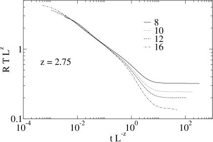
Figure 8: Finite size scaling collapse of MC data for the time dependent resistance function $R(t,T,L)$ with system sizes $L$ and temperatures $T$ related by $A=L^{1/\nu}T=0.8$. The data collapse is obtained for $\tau\sim L^{z}$ with $z=2.75$. Data for other values of $A$ scale with nearly the same value of $z$.

To reach further insight into the scaling properties at intermediate times we consider the order parameter autocorrelation function $G(t,T,L)$, defined in Eq. (9). Figure 9 shows MC data for $G(t,T,L)$ scaled according to Eq. (10) with $\tau\sim L^{z}$. The data in the figure has $L^{1/\nu}T=0.8$, and the data collapse is obtained for $z=2.74$. The data in the figure is for the case of fluctuating phase twists at the boundaries. We also calculated the same quantity with periodic boundary conditions, and obtained an equally good fit with the same exponent. Approximately the same exponent also gives a collapse for other values of $A$, but a slight drift in $z$ is noticeable, just as the data collapse in Fig. 3 for the RMS current is somewhat dependent on $A$. Including this uncertainty we estimate $z=2.7\pm 0.2$. We conclude that the dynamics measured by $G$ is independent of the phase twist fluctuations. The dynamic scaling relation $\tau\sim L^{2.7}$, instead comes from local dynamic fluctuations other than the global phase slips. This means that we can interpret the intermediate resistance scaling regime in Fig. 6 as coming from local fluctuations rather than global phase slips.

Figure 9: Finite size scaling data collapse of MC data for the dynamic correlation function $G(t,T,L)$ defined in Eq. (9).

VI Discussion and conclusions

This paper considers finite size scaling properties of Monte Carlo data for the glass transition in the two-dimensional gauge glass model. Equilibration of our simulations at low temperatures is achieved by a temperature exchange simulation method. Up to the level of statistical uncertainty, system sizes and temperatures reached in the simulations, our finite size scaling results for both static and dynamic properties show scaling properties that are clearly consistent with a glass transition occurring only at zero temperature, and thus indicates the absence of a superconducting glass state at any finite temperature in 2D.

Our results for static scaling properties reproduces, and adds some details to, some of the results of Refs. Katzgraber and Young, 2002; Katzgraber, 2003, in addition to providing a useful starting point for our dynamics simulations. From the scaling of the RMS current we find the correlation length exponent given by $1/\nu\approx 0.39$, obtained by optimizing the quality of a finite size scaling data collapse over a finite temperature interval close to $T=0$. This value agrees with that of Refs. Katzgraber and Young, 2002; Katzgraber, 2003. If we instead optimize the fit at the lowest temperatures where we have data, where scaling is also expected to work best, we obtain $1/\nu=0.36\pm 0.03$. It is interesting to note that this is in very good agreement with the result for the ground state domain wall exponent $\theta=-1/\nu$ in Ref. Akino and Kosterlitz, 2002. To obtain an even more accurate estimate of $\nu$, data for lower temperatures and bigger system sizes is necessary. To converge such data would require a considerable increase in simulation efforts.

For the dynamic properties, we consider the linear resistance computed from the diffusion of the phase slip across the boundary of the system. Since the correlation times grow very long at low temperature, it is not possible to converge the simulation at as low temperature as for the static data where the temperature exchange algorithm helps considerably, which makes it more difficult to study dynamic scaling than static scaling. A further complication is that our data for the linear resistance shows more than one characteristic time scale. We identify the longest correlation time as the characteristic time scale for phase slip fluctuations across the sample. Unfortunately it is not possible to determine the correlation time uniquely from the data, since the interval of sizes and temperatures where we have data is too limited. All the forms $\tau\sim\exp KL^{\psi}/T$, $\tau\sim\exp K\ln L/T$, and $\tau\sim L^{z}$ can be made to approximately fit the data. To discriminate between the possible forms, data at lower $T$ and larger $L$ is needed, which is beyond the present calculation. However, a logarithmically growing phase slip barrier, with $\tau\sim\exp K\ln L/T$, gives a good fit to the data with $K\approx 0.56$. A qualitatively similar result was obtained in a zero temperature calculation of the phase slip barrier energy in Ref. Holme and Olsson, 2002. Since $R\sim\exp-KL^{\psi}/T$, of which the logarithmic barrier is a special case with $\psi=0$, a superconducting glass with zero resistance is obtained only for $T=0$. In other words the dynamic glass transition occurs at zero temperature.

Surprisingly, data for the time dependent resistance function $R(t,T,L)$ does not scale with the longest correlation time for intermediate times. Instead, in this regime scaling is obtained by assuming a new correlation time of the form $\tau\sim L^{z}$ with $z=2.7\pm 0.2$. Hence the scaling behavior of our data implies two different diverging correlation times with quite different properties at the zero temperature glass transition. A further indication of the smaller correlation time is given by the scaling of the order parameter autocorrelation function, which scales over the entire time interval where we have data, including the longest times, quite in contrast to the resistance. The interpretation of this shorter correlation time is that it gives the characteristic time scale for fluctuations other than the global phase slip fluctuations that lead to a finite resistance. Similar results showing different dynamics for local fluctuations and phase twist fluctuations have been obtained previously at the finite temperature transition in XY models without disorder Jensen et al. (2000). We also note that the scaling relation $\tau\sim L^{z}$ can be written $\tau\sim\exp z\ln L\sim\exp zL^{0}\sim\exp C/T^{1+\psi\nu}$, which means that $\psi=\theta=-1/\nu$. Hence the relation $\tau\sim L^{z}$ suggests that the static and dynamic free energy barrier exponents are the same for the local fluctuations of the order parameter.

The two different diverging correlation times suggested here may explain why signatures of a glass phase with zero resistance at finite temperatures can easily be obtained in simulations. For the shorter correlation time we have $\psi=\theta=-1/\nu$, which gives $R(T)\sim\exp-C/T^{1+\psi\nu}=const$, for the resistance at small temperatures, i.e.  the resistance stays at the $T=0$ value $R=0$ for small $T$. This shows that in a regime of intermediate time scales, zero resistance can be obtained at finite temperature. However, at much longer time scales that may be hard to reach in a simulation, phase slip fluctuation set in, and qualitatively different behavior follows with a superconducting glass transition only at zero temperature.

In summary, from finite size scaling of a time dependent resistance function and an order parameter autocorrelation function, we constructed two different diverging correlation times from the $T_{c}=0$ scaling behavior of Monte Carlo data. For further work, it would be of interest to further clarify the precise details of dynamic scaling at the zero temperature glass transition, and to include quantum fluctuations in the model. It would furthermore be interesting to search for the proposed novel dynamic scaling behavior in experiments.

We acknowledge very helpful discussions with Petter Minnhagen, Helmut Katzgraber, Peter Olsson, Stephen Teitel, and Peter Young. This work was supported by the Swedish Research Council, PDC, NSC, and the Göran Gustafsson foundation.

References

- Fisher (1989) M. P. A. Fisher, Phys. Rev. Lett. 62, 1415 (1989).
- Lidmar (2003) J. Lidmar, Phys. Rev. Lett. 91, 097001 (2003).
- Katzgraber and Young (2002) H. Katzgraber and A. P. Young, Phys. Rev. B 66, 224507 (2002).
- Reger et al. (1991) J. D. Reger, T. A. Tokuyasu, A. P. Young, and M. P. A. Fisher, Phys. Rev. B 44, 7147 (1991).
- Olson and Young (2000) T. Olson and A. P. Young, Phys. Rev. B 61, 12467 (2000).
- Nishimori (1994) H. Nishimori, Physica A 205, 1 (1994).
- Bokil and Young (1995) H. S. Bokil and A. P. Young, Phys. Rev. Lett. 74, 3021 (1995).
- Akino and Kosterlitz (2002) N. Akino and J. M. Kosterlitz, Phys. Rev. B 66, 054536 (2002).
- Holme and Olsson (2002) P. Holme and P. Olsson, Europhys. Lett. 60, 439 (2002).
- Katzgraber (2003) H. G. Katzgraber, Phys. Rev. B 67, 180402(R) (2003).
- Holme et al. (2003) P. Holme, P. Minnhagen, and B. J. Kim, Phys. Rev. B 67, 104510 (2003).
- Choi and Park (1999) M. Y. Choi and S. Y. Park, Phys. Rev. B 60, 4070 (1999).
- Hyman et al. (1995) R. A. Hyman, M. Wallin, M. P. A. Fisher, S. M. Girvin, and A. P. Young, Phys. Rev. B 51, 15304 (1995).
- Wengel and Young (1996) C. Wengel and A. P. Young, Phys. Rev. B 54, 6869(R) (1996).
- Li (1992) Y.-H. Li, Phys. Rev. Lett. 69, 1819 (1992).
- Kim (2000) B. J. Kim, Phys. Rev. B 62, 644 (2000).
- Katzgraber and Campbell (2004) H. G. Katzgraber and I. A. Campbell, Phys. Rev. B 69, xxxx (2004).
- Hukushima and Nemoto (1996) K. Hukushima and K. Nemoto, J. Phys. Soc. Jpn. 65, 1604 (1996).
- Marinari (1998) E. Marinari, in Advances in Computer Simulation, edited by J. Kertész and I. Kondor (Springer-Verlag, 1998), p. 50.
- Shih et al. (1984) W. Y. Shih, C. Ebner, and D. Stroud, Phys. Rev. B 30, 134 (1984).
- Huse and Seung (1990) D. A. Huse and H. S. Seung, Phys. Rev. B 42, 1059 (1990).
- Fisher et al. (1991) D. S. Fisher, M. P. A. Fisher, and D. A. Huse, Phys. Rev. B 43, 130 (1991).
- Lidmar et al. (1998) J. Lidmar, M. Wallin, C. Wengel, S. Girvin, and A. Young, Phys. Rev. B 58, 2827 (1998).
- Young (1994) A. P. Young, in Random Magnetism, High-Temperature Superconductivity, edited by W. P. Beyermann, N. L. Huang-Liu, and D. E. MacLaughlin (World Scientific, Singapore, 1994), p. 113.
- Newman and Barkema (1999) M. E. J. Newman and G. T. Barkema, Monte Carlo Methods in Statistical Physics (Oxford University Press, 1999).
- Jensen et al. (2000) L. M. Jensen, B. J. Kim, and P. Minnhagen, Phys. Rev. B 61, 15412 (2000).