Weak localization in multiterminal networks of diffusive wires

Abstract

We study the quantum transport through networks of diffusive wires connected to reservoirs in the Landauer-Büttiker formalism. The elements of the conductance matrix are computed by the diagrammatic method. We recover the combination of classical resistances and obtain the weak localization corrections. For arbitrary networks, we show how the cooperon must be properly weighted over the different wires. Its nonlocality is clearly analyzed. We predict a new geometrical effect that may change the sign of the weak localization correction in multiterminal geometries.

^(a)Laboratoire de Physique Théorique et Modèles Statistiques. Université Paris-Sud, Bât. 100, F-91405 Orsay Cedex, France.

^(b)Laboratoire de Physique des Solides. Université Paris-Sud, Bât. 510, F-91405 Orsay Cedex, France.

PACS : 73.23.-b ; 73.20.Fz ; 72.15.Rn

How to increase transmission with weak localization ? This is one the question addressed in this letter devoted to a general description of transport in networks of quasi-one-dimensional weakly disordered wires. At the classical level, the network is equivalent to a network of classical resistances, which gives the dominant contribution to the conductances. Additionally, there exists a small correction, the “weak localization” correction, originating from quantum interferences. For the conductivity, it reads [2, 3] : $\Delta\sigma(\vec{r})=-\frac{e^{2}}{\pi}P_{c}(\vec{r},\vec{r})$ (with $\hbar=1$, without spin factor), where the cooperon $P_{c}$ is the contribution from pairs of time reversed trajectories to the return probability. Networks are particularly well suited to study interference effects and the first experimental studies of weak localization in such systems, performed on honeycomb lattices [4], showed the oscillations predicted by Altshuler-Aronov-Spivak (AAS) [5]. These experimental results were well fitted by the theory of Douçot & Rammal (DR) [6] whose starting point is a uniform integration of $\Delta\sigma(\vec{r})$ over the wires of the network [7]. However, although this procedure is meaningful for a translation invariant system, it is not valid in general for networks. In this letter we demonstrate that the correct expression of the weak localization correction to the resistance ${\cal R}$ of a network of wires $(\mu\nu)$ of lengths $l_{\mu\nu}$ and section $s$ is instead :

$$\Delta{\cal R}=\sum_{(\mu\nu)}\frac{\partial{\cal R}^{\rm cl}}{\partial R_{\mu\nu}^{\rm cl}}\Delta R_{\mu\nu}\mbox{ with }\frac{\Delta R_{\mu\nu}}{R^{\rm cl}_{\mu\nu}}=\int_{(\mu\nu)}{{\rm d}\vec{r}}\,\frac{-\Delta\sigma(\vec{r})}{s\,l_{\mu\nu}\,\sigma_{0}}$$ (1)

where ${\cal R}^{\rm cl}$ is the classical resistance obtained from the classical laws of combination of resistances $R^{\rm cl}_{\mu\nu}$. The sum runs over all wires $(\mu\nu)$. $\sigma_{0}$ is the Drude conductivity. This result has a simple structure : it could be obtained from small variations $\Delta R_{\mu\nu}$ in the classical expression ${\cal R}^{\rm cl}$ of the resistance. However it is highly non trivial since, due to nonlocality, it is not possible to get a quantum formula for the resistance of the network as a function of quantum resistances of the wires. It is in fact not even possible to define a quantum resistance for a wire, independently of the whole network. Eq. (1) shows that a uniform integration of the cooperon is applicable only to regular networks in which the weights of the wires $\partial{\cal R}^{\rm cl}/\partial R_{\mu\nu}^{\rm cl}$ are all equal, like in the experiments of Ref. [4]. We show that in a multiterminal geometry, some of these weights can change in sign. This can lead to a change in sign of the weak localization correction.

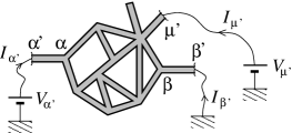
FIG. 1.: A network of diffusive wires. The network is connected at the vertices $\alpha^{\prime}$, $\beta^{\prime}$ and $\mu^{\prime}$ to external reservoirs through which some current is injected in the network.

As on figure 1, we consider networks that can be connected to external contacts (here the contacts $\alpha^{\prime}$, $\beta^{\prime}$ and $\mu^{\prime}$). The transmission probability between two contacts (the conductance matrix element, up to a factor $e^{2}/h$), when averaged over the disorder, can be written as $\langle T_{\alpha^{\prime}\beta^{\prime}}\rangle=T^{\rm cl}_{\alpha^{\prime}\beta^{\prime}}+\Delta T_{\alpha^{\prime}\beta^{\prime}}+\cdots$, where the first term is the classical result (Drude conductance) and the second is the weak localization correction. Our aim is to give a systematic way to compute the weak localization contribution in terms of matrices encoding the information on the network (topology, lengths of the wires, magnetic fluxes). The most natural approach to describe transport in networks is the Landauer-Büttiker approach. However some difficulties related to the question of current conservation are more conveniently overcome in the Kubo formulation. We first recall some features of the transport theory of weakly disordered metals in the Kubo approach and eventually use the connection to the Landauer-Büttiker formalism that we apply to the case of networks. Finally we consider several examples.

Classical transport. The classical transport is described by two contributions : a Drude contribution (short range) and the contribution from the diffuson (ladder diagrams) which is long range. Then, in the diffusion approximation, we have [10] :

$$\langle\sigma_{ij}(\vec{r},\vec{r}\,^{\prime})\rangle_{\rm class}=\raisebox{-11.38092pt}{\includegraphics[scale={0.5}]{sigdrude.eps}}+\raisebox{-17.07182pt}{\includegraphics[scale={0.5}]{sigdiffuson2.eps}}$$ (2)

$$=\sigma_{\rm 0}\,\left[\delta_{ij}\>{\delta}(\vec{r}-\vec{r}\,^{\prime})-\nabla_{i}\nabla^{\prime}\!\!_{j}P_{d}(\vec{r},\vec{r}\,^{\prime})\right]=\sigma_{\rm 0}\>\phi_{ij}(\vec{r},\vec{r}\,^{\prime})\>,$$ (3)

where the diffuson $P_{d}$ is solution of the equation $-\Delta P_{d}(\vec{r},\vec{r}\,^{\prime})=\delta(\vec{r}-\vec{r}\,^{\prime})$. An important requirement of a transport theory is to satisfy current conservation $\nabla_{i}\sigma_{ij}(\vec{r},\vec{r}\,^{\prime})=0$, what the classical conductivity (2) does. The question of boundary conditions is not a trivial one. In most works, it is argued, by analogy with the problem of classical diffusion, that $\vec{n}\cdot\vec{\nabla}P_{d}|_{\partial{\cal D}}=0$ on the reflecting boundaries of the domain ${\cal D}$ ($\vec{n}$ is the vector normal to the surface), while $P_{d}|_{\partial{\cal D}}=0$ on the boundaries where the disordered system is connected to a reservoir. This latter is described by a region free of disorder. However it was shown in [11, 12, 13] that the diffuson vanishes at a distance of order $\ell_{e}$ inside the reservoir. $\ell_{e}$ is the elastic mean free path. In the case of a quasi-1d wire, the diffuson vanishes at a distance $x_{d}=\alpha_{d}\ell_{e}/2$, where $d$ is the dimension with $\alpha_{1}=2$, $\alpha_{2}=\pi/2$, $\alpha_{3}=4/3$.

Current conserving weak localization correction. The weak localization correction involves the cooperon which, in a magnetic field $\vec{\cal B}=\vec{\nabla}\times\vec{A}$, is solution of :

$$\left[\frac{1}{L_{\varphi}^{2}}-\left(\vec{\nabla}-2{\rm i}e\vec{A}\right)^{2}\right]P_{c}(\vec{r},\vec{r}\,^{\prime})=\delta(\vec{r}-\vec{r}\,^{\prime})\>.$$ (4)

The contribution of the cooperon reads [2, 3] :

$$\langle\sigma_{ij}(\vec{r},\vec{r}\,^{\prime})\rangle_{\rm cooperon}=\raisebox{-17.07182pt}{\includegraphics[scale={0.5}]{sigcooperon2.eps}}$$ (5)

$$\hskip 28.45274pt=-\frac{e^{2}}{\pi}\,\delta_{ij}\,\delta(\vec{r}-\vec{r}\,^{\prime})\,P_{c}(\vec{r},\vec{r})\>.$$ (6)

It is clear that the additional contribution of the cooperon (5) does not respect current conservation. In the same way that the classical conductivity is built of short range (Drude) and long range (diffuson) contributions, the weak localization correction contains long range terms additionally to the short range contribution (5). A possible way to build a long range diagram is to dress the current vertices with diffusons, like on figure 2.

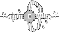
FIG. 2.: A long range diagram for the weak localization.

The connection of the cooperon and the diffusons is realized by introducing a Hikami box [14]. Dressing either the left current line with a diffuson, or the right one or both, we obtain three diagrams that add to the contribution of the cooperon. However these dominant diagrams are not the only ones needed to satisfy current conservation [12]. This is related to the fact that the diagram 2, which seems at first sight to be the only long range diagram needed to compute the weak localization, gives a volumic divergence $V\delta(0)$ to the conductance (for details, see [15]). This problem was first mentioned in the study of conductivity fluctuations [10] where a more simple procedure to construct a current conserving theory was proposed, that avoids to consider all the set of diagrams of [12]. Kane, Serota and Lee showed, for the conductivity fluctuations, that the expression of the current conserving conductivity is obtained by a “convolution” of the short range object with the function $\phi_{ij}$ involved in (2). Finally the expression of the weak localization correction to the nonlocal conductivity reads :

$$\langle\Delta\sigma_{ij}(\vec{r},\vec{r}\,^{\prime})\rangle=\int{\rm d}\vec{\rho}\,{\rm d}\vec{\rho}\,^{\prime}\,$$ (7)

$$\hskip 42.67912pt\phi_{ii^{\prime}}(\vec{r},\vec{\rho})\,\phi_{jj^{\prime}}(\vec{r}\,^{\prime},\vec{\rho}\,^{\prime})\,\langle\sigma_{i^{\prime}j^{\prime}}(\vec{\rho},\vec{\rho}\,^{\prime})\rangle_{\rm cooperon}\>,$$ (8)

which obviously respects current conservation.

Networks. We now consider specifically the case of networks such as the one on figure 1. The transmission $T_{\alpha^{\prime}\beta^{\prime}}$ between the two contacts (conductance in unit $e^{2}/h$) is related to the nonlocal conductivity $\sigma_{ij}(\vec{r},\vec{r}\,^{\prime})$ with $\vec{r}$ being integrated through the section of the contact $\alpha^{\prime}$ and $\vec{r}\,^{\prime}$ through the section of the contact $\beta^{\prime}$ [16]. For quasi-1d wires, we obtain the expressions

$$T^{\rm cl}_{\alpha^{\prime}\beta^{\prime}}=\frac{\alpha_{d}N_{c}}{\ell_{e}}P_{d}(\underline{\alpha}^{\prime},\underline{\beta}^{\prime})$$ (9)

where $N_{c}$ is the number of channels in the wires, and

$$\Delta{T}_{\alpha^{\prime}\beta^{\prime}}=\frac{2}{\ell_{e}^{2}}\int_{\rm Network}{\rm d}x\,\frac{{\rm d}}{{\rm d}x}P_{d}(\underline{\alpha}^{\prime},x)\>P_{c}(x,x)\>\frac{{\rm d}}{{\rm d}x}P_{d}(x,\underline{\beta}^{\prime})\>,$$ (10)

that involve the one-dimensional diffuson and cooperon, solutions of the diffusion equation $\left[\gamma-{\rm D}_{x}^{2}\right]P(x,x^{\prime})=\delta(x-x^{\prime})$, where ${\rm D}_{x}={\rm d}_{x}-2{\rm i}eA(x)$ is the covariant derivative and $\gamma=1/L_{\varphi}^{2}$ (for $P_{d}$ we set $\gamma=0$ and $A(x)=0$). The notation $P_{d}(\underline{\alpha}^{\prime},x)$ means that the diffuson is taken at a distance $\ell_{e}$ of the vertex $\alpha^{\prime}$. Eq. (9,10) assume Dirichlet boundary conditions at the vertices connected to reservoirs. Indeed, it can be shown that the correct boundary conditions mentioned above can be replaced by $P_{d}|_{\partial{\cal D}}=0$, providing to insert a multiplicative factor $4$, independent of $d$, as it has been done in (9,10). This simplifies slightly the calculations.

As a check, let us consider the case of a quasi-1d wire of length $L$ connected to reservoirs at both sides. We recover the Drude dimensionless conductance $g_{\rm D}=\alpha_{d}N_{c}\ell_{e}/L$, and the correction $\Delta g=-\frac{L_{\varphi}}{L}\big{(}\coth\frac{L}{L_{\varphi}}-\frac{L_{\varphi}}{L}\big{)}$ which interpolates between $\Delta g=-1/3$ in the fully coherent limit ($L\ll L_{\varphi}$), and $\Delta g=-L_{\varphi}/L$ for $L\gg L_{\varphi}$.

We introduce the adjacency matrix $a_{\alpha\beta}$ that encodes the information on the topology of the network : $a_{\alpha\beta}=1$ if the vertices $\alpha$ and $\beta$ are connected by a wire $(\alpha\beta)$, whose length is denoted by $l_{\alpha\beta}$; $a_{\alpha\beta}=0$ otherwise. To construct the solution of the diffusion equation, we need to specify boundary conditions at the vertices. We impose continuity of $P$ and $\sum_{\beta}a_{\alpha\beta}P^{\prime}_{({\alpha\beta})}(\alpha)=\lambda_{\alpha}P(\alpha)$ : the adjacency matrix constrains the sum to run over the neighbouring vertices of $\alpha$. The parameters $\lambda_{\alpha}$ describe how the network is connected. $\lambda_{\alpha}=0$ for an internal vertex and $\lambda_{\alpha}=\infty$ at the vertices connected to external reservoirs, which imposes a Dirichlet boundary condition. The solution for $P_{c}$ involves the matrix [6, 8, 9, 15] :

$${\cal M}_{\alpha\beta}= \delta_{\alpha\beta}\left(\lambda_{\alpha}+\sqrt{\gamma}\sum_{\mu}a_{\alpha\mu}\coth(\sqrt{\gamma}l_{\alpha\mu})\right)$$ (12)

$$\hskip 28.45274pt-a_{\alpha\beta}\frac{\sqrt{\gamma}\>{\mbox{e}}^{-{\rm i}\theta_{\alpha\beta}}}{\mathop{\mathrm{sh}}\nolimits(\sqrt{\gamma}l_{\alpha\beta})}\>.$$

The diffuson is expressed in terms of the same matrix with $\gamma=0$ and no magnetic flux $\theta_{\alpha\beta}=0$ :

$$\left({\cal M}_{0}\right)_{\alpha\beta}=\delta_{\alpha\beta}\left(\lambda_{\alpha}+\sum_{\mu}a_{\alpha\mu}\frac{1}{l_{\alpha\mu}}\right)-a_{\alpha\beta}\frac{1}{l_{\alpha\beta}}\>.$$ (13)

This matrix encodes the information about the classical conductances $\alpha_{d}N_{c}\ell_{e}/l_{\mu\nu}$ of each wire $(\mu\nu)$. Note that $\lambda_{\alpha^{\prime}}=\infty$ (at a reservoir) implies that $({\cal M}^{-1})_{\mu\alpha^{\prime}}=0$, $\forall$ $\mu$. The classical conductance is given by

$$T^{\rm cl}_{\alpha^{\prime}\beta^{\prime}}=\frac{\alpha_{d}N_{c}\ell_{e}}{l_{\alpha\alpha^{\prime}}l_{\beta\beta^{\prime}}}\left({\cal M}_{0}^{-1}\right)_{\alpha\beta}\>.$$ (14)

This result is only valid for $\alpha^{\prime}\neq\beta^{\prime}$ [12]. It coincides with the one obtained for a network of classical resistances, as it should.

In Eq. (10), we separate the integral over the network into contributions of the different wires : $\int_{\rm Network}\to\sum_{(\mu\nu)}\int_{(\mu\nu)}$. Since the diffuson $P_{d}(\underline{\alpha}^{\prime},x)$ is linear in $x$ on the wire $(\mu\nu)$, the derivatives produce coefficients depending on $(\mu\nu)$ :

$$\frac{{\rm d}}{{\rm d}x}P_{d}(\underline{\alpha}^{\prime},x\in(\mu\nu))=\frac{\ell_{e}}{l_{\alpha\alpha^{\prime}}l_{\mu\nu}}$$ (15)

$$\times\left[-\left({\cal M}_{0}^{-1}\right)_{\alpha\mu}\,+\left({\cal M}_{0}^{-1}\right)_{\alpha\nu}+\delta_{\mu\alpha}\delta_{\nu\alpha^{\prime}}\,l_{\alpha\alpha^{\prime}}\right]\>.$$ (16)

Replacing (15) in (10) shows explicitly the non trivial weights that should be attributed to each wire when integrating the cooperon over the wires. These weights have a clear physical meaning : they can be related to derivatives of the corresponding classical conductance with respect to the lengths of the wires. From (10,14,15) we obtain :

$$\Delta T_{\alpha^{\prime}\beta^{\prime}}=\frac{2}{\alpha_{d}N_{c}\ell_{e}}\sum_{(\mu\nu)}\frac{\partial T^{\rm cl}_{\alpha^{\prime}\beta^{\prime}}}{\partial\,l_{\mu\nu}}\int_{(\mu\nu)}{\rm d}x\,P_{c}(x,x)\>.$$ (17)

We have demonstrated (1), since $\sigma_{0}=\frac{e^{2}\alpha_{d}N_{c}\ell_{e}}{2\pi\,s}$.The integral of the cooperon over the bond $(\mu\nu)$ is a nonlocal quantity that carries information on the whole structure of the network through the matrix ${\cal M}^{-1}$ :

$$\int_{(\mu\nu)}{\rm d}x\,P_{c}(x,x)=\frac{1}{2\sqrt{\gamma}}\bigg{\{}\left[\left({\cal M}^{-1}\right)_{\mu\mu}+\left({\cal M}^{-1}\right)_{\nu\nu}\right]\left(\coth\sqrt{\gamma}l_{\mu\nu}-\frac{\sqrt{\gamma}l_{\mu\nu}}{\mathop{\mathrm{sh}}\nolimits^{2}\sqrt{\gamma}l_{\mu\nu}}\right)$$ (18)

$$+\left[\left({\cal M}^{-1}\right)_{\mu\nu}{\mbox{e}}^{{\rm i}\theta_{\mu\nu}}+\left({\cal M}^{-1}\right)_{\nu\mu}{\mbox{e}}^{{\rm i}\theta_{\nu\mu}}+\frac{\mathop{\mathrm{sh}}\nolimits\sqrt{\gamma}l_{\mu\nu}}{\sqrt{\gamma}}\right]\frac{-1+\sqrt{\gamma}l_{\mu\nu}\coth\sqrt{\gamma}l_{\mu\nu}}{\mathop{\mathrm{sh}}\nolimits\sqrt{\gamma}l_{\mu\nu}}\bigg{\}}\>.$$ (19)

Eqs. (17,18) give the weak localization correction for any network. We now turn to few special cases.

Incoherent networks. If all wires are longer than the phase coherence length ($l_{\mu\nu}\gg L_{\varphi}$, $\forall$ $(\mu\nu)$), the weak localization correction (17) involves the same length as the classical conductance (14). If we write $T^{\rm cl}_{\alpha^{\prime}\beta^{\prime}}={\alpha_{d}N_{c}\ell_{e}}/L_{\rm eff}$, then

$$\Delta{T}_{\alpha^{\prime}\beta^{\prime}}\simeq-\frac{L_{\varphi}}{l_{\alpha\alpha^{\prime}}l_{\beta\beta^{\prime}}}\left({\cal M}_{0}^{-1}\right)_{\alpha\beta}=-\frac{L_{\varphi}}{L_{\rm eff}}\>.$$ (20)

The ratio $\Delta{T}_{\alpha^{\prime}\beta^{\prime}}/T^{\rm cl}_{\alpha^{\prime}\beta^{\prime}}$ is network independent in this case. This simple result strongly relies on the hypothesis of wires with equal sections [15].

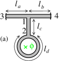
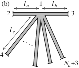
FIG. 3.: Two examples of mesoscopic devices. The wavy lines indicate connection to external reservoirs.

A ring. The transport through a ring has been studied in [17]. Here we rather consider the device on figure 3.a to illustrate the nonlocality of the weak localization. The classical conductance (14) is $T^{\rm cl}_{34}=\frac{\alpha_{d}N_{c}\ell_{e}}{l_{a}+l_{b}}$. It is independent of the presence of the arm and the ring. Then their weights are 0 and this part of the network does not contribute to the weak localization correction (17). However, since the cooperon $P_{c}(x,x)$ is nonlocal, it feels the presence of the loop, even for $x$ in the wires $(3\leftrightarrow 1)$ and $(1\leftrightarrow 4)$. Note that the naive uniform integration of the cooperon over the network (DRPM) strongly overestimates the amplitude of the AAS oscillations (figure 4) [15]. The decrease of the weak localization at high field (inset) is due to the contribution of the flux to the effective phase coherence length $L_{\varphi}(\phi)$ [18].

FIG. 4.: Dashed line : $\Delta\sigma/\sigma_{0}$ for a uniform integration of $P_{c}$. Continuous line : $\Delta T_{34}/T^{\rm cl}_{34}$ given by (17). The curves have been shifted so that they coincide at $\phi=0$. Inset : Same curves (without shift) for a higher window of flux $\phi$. The parameters are $l_{a}=l_{b}=1\>\mu$m, $l_{c}=0.05\>\mu$m and $l_{d}=5\>\mu$m. $W=0.19\>\mu$m, $L_{\varphi}(\phi=0)=1.7\>\mu$m.

Multiterminal geometry. The origin of the negative weak localization $\Delta T_{\alpha^{\prime}\beta^{\prime}}$ lies in the negative weights, however for a multiterminal geometry some weights can be positive, like the weight(s) $\partial{T^{\rm cl}_{\alpha^{\prime}\beta^{\prime}}}/\partial{l_{\mu\mu^{\prime}}}$ of the wire(s) connected to other terminal(s) (e.g. $\mu^{\prime}$ on figure 1). As a first example, we consider a wire on which is plugged one long arm of length $l_{c}$ connected to a third reservoir (figure 3.b for $N_{a}=1$). We focus ourselves on the fully coherent limit $L_{\varphi}=\infty$. The classical (Drude) conductance of this 3-terminal network is : $T^{\rm cl}_{23}=\frac{\alpha_{d}N_{c}\ell_{e}\,l_{c}}{l_{a}l_{b}+l_{b}l_{c}+l_{c}l_{a}}$. Then ${\partial T^{\rm cl}_{23}}/{\partial l_{c}}>0$. The wire [$(2\leftrightarrow 1)+(1\leftrightarrow 3)$] gives a negative contribution to the weak localization correction whereas the arm $(1\leftrightarrow 4)$ gives a positive one. Introducing $l_{a/\!/b/\!/c}^{-1}=l_{a}^{-1}+l_{b}^{-1}+l_{c}^{-1}$, we find

$$\Delta T_{23}=\frac{1}{3}\left(-1+\frac{l_{a/\!/b/\!/c}}{l_{c}}+\frac{l_{a/\!/b/\!/c}^{2}}{l_{a}l_{b}}\right)\simeq\frac{1}{3}\left(-1+\frac{l_{a/\!/b}}{l_{a}+l_{b}}\right)$$

in the limit $l_{a/\!/b}\ll l_{c}$. We now consider the case of $N_{a}$ long arms plugged in the middle of the wire ($l_{a}=l_{b}$) like on figure 3.b , to maximize their effect [15]. We obtain :

$$\Delta T_{23}\simeq\frac{1}{3}\left(-1+\frac{N_{a}}{4}\right)\>,$$ (21)

a result valid for $l_{a}\ll l_{c}\ll L_{\varphi}$. We can now obtain a positive weak localization correction for $N_{a}>4$. This effect is purely geometrical. Note that in the limit $l_{c}\gg L_{\varphi}$ the positive contribution vanishes.

Conclusion. We have provided a general theory for the quantum transport of networks of diffusive wires connected to reservoirs. We obtained the classical conductances and the weak localization corrections. We emphasized the importance of the weights to give to the wires when integrating the cooperon over the network. This can lead to new geometrical effects like a positive correction (21), the physical reason being that coherent backscattering in a multiterminal geometry can enhance a transmission.

REFERENCES

[1]
[2]
L. P. Gor’kov, A. I. Larkin, and D. E. Khmel’nitzkiĭ,
JETP Lett. 30, 228 (1979).
[3]
B. L. Al’tshuler, D. E. Khmel’nitzkiĭ, A. I. Larkin, and P. A. Lee,
Phys. Rev. B 22, 5142 (1980).
[4]
B. Pannetier, J. Chaussy, R. Rammal, and P. Gandit,
Phys. Rev. Lett. 53, 718 (1984);
Phys. Rev. B 31, 3209 (1985).
[5]
B. L. Al’tshuler, A. G. Aronov, and B. Z. Spivak,
JETP Lett. 33, 94 (1981).
[6]
B. Douçot and R. Rammal,
Phys. Rev. Lett. 55, 1148 (1985);
J. Physique 47, 973 (1986).
[7]
The theory of DR [6] was made more efficient in [8]
(PM) by finding a simple way to express the integral of the cooperon over
the network (see also [9]).
PM considered thermodynamic properties for which it is correct to integrate
the cooperon uniformly over the network.
[8]
M. Pascaud and G. Montambaux,
Phys. Rev. Lett. 82, 4512 (1999).
[9]
E. Akkermans, A. Comtet, J. Desbois, G. Montambaux, and C. Texier,
Ann. Phys. (N.Y.) 284, 10 (2000).
[10]
C. L. Kane, R. A. Serota, and P. A. Lee,
Phys. Rev. B 37, 6701 (1988).
[11]
A. Ishimaru,
Wave propagation and scattering in random media,
Academic Press, New York, 1978.
[12]
M. B. Hastings, A. D. Stone, and H. U. Baranger,
Phys. Rev. B 50, 8230 (1994).
[13]
E. Akkermans and G. Montambaux,
Physique Mésoscopique des électrons et des
photons,
CNRS-Intereditions, 2004, to appear.
[14]
S. Hikami,
Phys. Rev. B 24, 2671 (1981).
[15]
C. Texier, G. Montambaux, and E. Akkermans,
in preparation (2004).
[16]
H. U. Baranger and A. D. Stone,
Phys. Rev. B 40, 8169 (1989).
[17]
P. Santhanam,
Phys. Rev. B 39, 2541 (1989).
[18]
B. L. Al’tshuler and A. G. Aronov,
JETP Lett. 33, 499 (1981).