Averaging For Solitons With Nonlinearity Management

Abstract

We develop an averaging method for solitons of the nonlinear Schrödinger equation with periodically varying nonlinearity coefficient. This method is used to effectively describe solitons in Bose-Einstein condensates, in the context of the recently proposed and experimentally realizable technique of Feshbach resonance management. Using the derived local averaged equation, we study matter-wave bright and dark solitons and demonstrate a very good agreement between solutions of the averaged and full equations.

Introduction. Dispersive nonlinear wave equations are appropriate mathematical models for various nonlinear phenomena in fluid mechanics, optics, plasmas and condensed matter physics. The prototypical equation that generically emerges in the description of envelope waves is the nonlinear Schrödinger (NLS) equation [1, 2, 3] of the form:

$$iu_{t}=-D\Delta u+\Gamma|u|^{2}u+V({\bf x})u.$$ (1)

Here $u({\bf x},t)$ is a complex envelope field, $V({\bf x})$ is an external potential, $\Delta$ is the Laplacian operator in multi dimensions, and $D$ and $\Gamma$ are the coefficients of the dispersive and nonlinear terms respectively.

In a number of physical applications, the coefficients $D$ and $\Gamma$ exhibit temporal periodic variations. When $D=D(t)$, the NLS equation (1) describes the dispersion management (DM) scheme in fiber optics, which is based on periodic alternation of fibers with opposite signs of the group-velocity dispersion. The DM scheme supports robust breathing solitons [4], which are well described through the averaging method by the integral NLS equation [5]. Extensions of the averaging method were developed for strong management with large variations of the dispersion coefficient [6] and for weak management with small variations of the dispersion coefficient [7].

When $\Gamma=\Gamma(t)$, the NLS equation (1) has applications in optics for transverse beam propagation in layered optical media [8], as well as in atomic physics for the Feshbach resonance [9] of the scattering length of inter-atomic interactions in Bose-Einstein condensates (BECs). The periodic variation of the scattering length by means of an external magnetic field provides an experimentally realizable protocol for the generation of robust matter-wave breathers [10], and for their persistence against collapse type phenomena in higher dimensions [11, 12]. Solitary waves have become a focal point in studies of BEC both theoretically and experimentally [13, 14] due to their coherence properties. Hence, nonlinearity management using Feshbach resonance promises to provide a viable alternative for the generation of coherent nonlinear wave structures.

Given the importance in nonlinear optics and condensed matter physics, of applications of the NLS equation (1) with periodically varying nonlinearity coefficient, we extend the averaging method of [5, 6] to solitons with strong nonlinearity management, when the periodic variations of the nonlinearity coefficient are large in amplitude. Comparing with earlier works, we note that the averaged equation for strong dispersion management in [5, 6] is nonlocal, whereas our main averaged equation (see Eq. (14)) for strong nonlinearity management is local. Furthermore, our averaging method is more general than the asymptotic expansion method, exploited for weak dispersion management in [7] and for weak nonlinearity management in [11]. Since the averaged equation obtained herein is simple, we compute numerically solitary waves of the averaged equation and compare with those of the full problem, showing the excellent agreement between the two.

We emphasize that the main contribution of this work is two-fold. From a mathematical point of view, it is the derivation of a novel averaged equation that describes dynamics of solitary waves under nonlinearity management. From a physical point of view, the main result is the computation of the parameter domains, where nonlinear waves exist in the BEC and nonlinear optics. We hope that highlighting the relevant analogies and differences may also stimulate additional cross-fertilization between these sub-disciplines and their respective mathematical techniques. Furthermore, our work poses the interesting problem of understanding what happens in the parameter domains, where solitary waves do not exist. These fundamental problems are of interest not only to theorists and experimentalists in atomic and optical physics but also, more generally, to researchers in nonlinear and wave physics, where periodic temporal variations and their averaging methods are studied (see e.g., [15]).

Derivation of the averaged equation. We start with the NLS equation (1) with $D=1$ and $\Gamma=\Gamma(t)$. The external potential $V(x)$ is left arbitrary but we keep in mind that the magnetic and laser trappings relevant to BEC applications impose parabolic and periodic potentials respectively. Also, we will restrict ourselves to one spatial dimension, but generalization of the method to multi-dimensions is straightforward. The resulting equation (also referred to as the Gross–Pitaevskii (GP) equation [3]) describes the “cigar-shaped” BECs and reads:

$$iu_{t}=-u_{xx}+\Gamma(t)|u|^{2}u+V(x)u,$$ (2)

where the nonlinearity coefficient (proportional to the scattering length in the BECs) $\Gamma(t+\epsilon)=\Gamma(t)$ is a smooth, sign-indefinite, periodic function of period $\epsilon$. We assume that the period $\epsilon$ of the nonlinearity management is small compared to the characteristic propagation time of nonlinear waves, while the nonlinearity variations are large in amplitude. In this case, we decompose $\Gamma(t)$ into the mean-value part $\gamma_{0}$ and a large fast-varying part $\gamma$, according to the representation:

$$\Gamma(t)=\gamma_{0}+\frac{1}{\epsilon}\gamma(\tau),\qquad\tau=\frac{t}{\epsilon},$$ (3)

where $\gamma(\tau+1)=\gamma(\tau)$ and $\int_{0}^{1}\gamma(\tau)d\tau=0$. Using

$$u(x,t)=v(x,\tau)\exp\left(-i\int_{0}^{\tau}\gamma(\tau^{\prime})|v|^{2}(x,\tau^{\prime})d\tau^{\prime}\right),$$ (4)

we remove the large fast variations of the nonlinearity coefficient and bring the GP equation (2) to an equivalent form:

$$i\epsilon^{-1}v_{\tau}=-v_{xx}+\gamma_{0}|v|^{2}v+V(x)v$$ (5)

$$+2iv_{x}\int_{0}^{\tau}\gamma(\tau^{\prime})|v|^{2}_{x}(x,\tau^{\prime})d\tau^{\prime}+iv\int_{0}^{\tau}\gamma(\tau^{\prime})|v|^{2}_{xx}(x,\tau^{\prime})d\tau^{\prime}$$ (6)

$$+v\left(\int_{0}^{\tau}\gamma(\tau^{\prime})|v|^{2}_{x}(x,\tau^{\prime})d\tau^{\prime}\right)^{2}.$$ (7)

In the averaging method (see [6] for details), we decompose solutions of the problem with variable coefficients (7) into a slowly varying mean part $w(x,t)$ and a small, fast-varying part $v_{1}(x,\tau)$:

$$v(x,\tau)=w(x,t)+\epsilon v_{1}(x,\tau;w(x,t)),\qquad t=\epsilon\tau.$$ (8)

The varying part $v_{1}(x,\tau;w)$ is a periodic function of $\tau$ with unit period. To leading order, this condition is satisfied if $w(x,t)$ satisfies the averaged equation:

$$iw_{t}= - w_{xx}+\gamma_{0}|w|^{2}w+V(x)w$$ (9)

$$+ 2i\nu_{1}w_{x}|w|^{2}_{x}+i\nu_{1}w|w|^{2}_{xx}+\nu_{2}w\left(|w|^{2}_{x}\right)^{2},$$ (10)

where $\nu_{1}=\int_{0}^{1}\nu(\tau)d\tau$, $\nu_{2}=\int_{0}^{1}\nu^{2}(\tau)d\tau$, and $\nu(\tau)=\int_{0}^{\tau}\gamma(\tau^{\prime})d\tau^{\prime}$. The averaging method is simplified with the gauge transformation,

$$w(x,t)=\psi(x,t)\exp\left(i\nu_{1}|\psi|^{2}(x,t)\right),$$ (11)

which reduces (9) to the form:

$$i\psi_{t}-\nu_{1}\psi|\psi|^{2}_{t}= - \psi_{xx}+\gamma_{0}|\psi|^{2}\psi+V(x)\psi$$ (12)

$$+ \mu\psi\left(|\psi|^{2}_{x}\right)^{2},$$ (13)

where $\mu=\nu_{2}-\nu_{1}^{2}$. Using the balance equation $i|\psi|^{2}_{t}=\left(\bar{\psi}_{x}\psi-\bar{\psi}\psi_{x}\right)_{x}$, which follows from (13), we rewrite the averaged equation in the final form:

$$i\psi_{t}= - \psi_{xx}+\gamma_{0}|\psi|^{2}\psi+V(x)\psi+\mu\psi\left(|\psi|^{2}_{x}\right)^{2}$$ (14)

$$+ i\nu_{1}\psi\left(\bar{\psi}\psi_{x}-\bar{\psi}_{x}\psi\right)_{x}.$$ (15)

The averaged equation (14) is the main result of this Letter. It is seen to be equivalent to the integral averaged equation derived for strong dispersion management in fiber optics [5, 6], but it is a local evolution equation. A similar local equation was also derived for weak dispersion management in fiber optics [7], when the last two terms of (14) are small compared to the leading-order NLS equation. We emphasize that our main averaged equation (14) is derived for strong nonlinearity management and it captures all terms in the same, leading order of the averaging method.

Solitons in BECs. The simplest standing waves of the averaged equation (14) are obtained through the standard ansatz [1]:

$$\psi(x,t)=\phi(x)e^{i\omega t},$$ (16)

where $\phi(x)$ solves the second-order differential equation:

$$-\phi^{\prime\prime}+\omega\phi+V(x)\phi+\gamma_{0}\phi^{3}+4\mu(\phi^{\prime})^{2}\phi^{3}=0.$$ (17)

As a typical example of a smooth periodic variation of the scattering length [11, 12], we use the sinusoidal function $\Gamma(t)=\gamma_{0}+\gamma_{1}\sin(2\pi t)$, in which case $\mu=\gamma_{1}^{2}/(8\pi^{2})$. We also set $\epsilon=1$ and choose $|\omega|\in[0.1,0.5]$ to ensure validity of the averaged equation (17), when $\epsilon\ll 2\pi/|\omega|$. We also use the parabolic potential $V(x)$ for the magnetic trapping of the BEC, $V(x)=\frac{1}{2}\Omega^{2}x^{2}$, where $\Omega^{2}\in[0.02,0.4]$.

To estimate actual physical quantities corresponding to the above values of the normalized parameters, we first note that the cases $\gamma_{0}<0$ ($\gamma_{0}>0$) are relevant to an attractive (repulsive) condensate, such as ⁷Li (⁸⁵Rb), characterized by a negative (positive) scattering length $a=-1$nm ($a=0.8$nm), in a magnetic field $B\approx 650$ G ($B\approx 159$ G). These values of the scattering lengths set the units in the parameters $\gamma_{0}$ and $\gamma_{1}$, which may take different values as long as the magnetic field $B$ is varied [9]. On the other hand, the number of atoms $N$ in the two condensates is taken to be as follows: $N=1\times 10^{4}$ ($N=2\times 10^{5}$) for $\Omega^{2}=0.4$ ($\Omega^{2}=0.02$) for the ⁷Li condensate and $N=4\times 10^{3}$ ($N=7.5\times 10^{4}$) for $\Omega^{2}=0.4$ ($\Omega^{2}=0.02$) for the ⁸⁵Rb condensate. Since we deal with cigar-shaped BECs, we may assume that the external magnetic trap is highly anisotropic, characterized by the confining frequencies $\omega_{\parallel}=2\pi\times 3.6$Hz and $\omega_{\perp}=2\pi\times 360$Hz in the axial and transverse directions respectively. In such a case, the time and space units in the results that will be presented below, are $44.2$ms and $2\mu$m (for ⁷Li) or $44.2$ms and $0.6\mu$m (for ⁸⁵Rb).

Numerical Results. Using Eq. (17), we can now obtain the solution $\phi(x)$ for a given set of parameters ($\gamma_{0},\gamma_{1},\Omega,\omega$), by means of the Newton method. We also perform parameter continuations, to follow the solution branches as the parameters vary.

Fig. 1 shows two solutions of the averaged equation (17) with $\gamma_{0}<0$ (the attractive BEC with negative scattering length), $\gamma_{1}=0.5$, $\Omega^{2}=0.4$, and $\omega=0.5$. The solution on the left panel is the bright soliton, which has the form $\phi(x)=(2\omega/\gamma_{0})^{1/2}{\rm sech}(\omega^{1/2}x)$ when $\gamma_{1}=\Omega=0$. The solution on the right panel is the so-called twisted soliton, which corresponds to a concatenation of two separated bright solitons of opposite parity (see e.g., [16]). The twisted soliton does not exist when $\gamma_{0}<0$ and $\Omega=0$. Higher-order solutions with multiple nodes (zeros) may also exist in the averaged equation (17) with $\gamma_{0}<0$ and $\Omega\neq 0$, in some parameter domains.

Fig. 2 shows two solutions of the averaged equation (17) with $\gamma_{0}>0$ (the repulsive BEC with positive scattering length), $\gamma_{1}=0.5$, and $\omega=-0.5$. In the case of $\gamma_{0}>0$, the localized solutions of Eq. (17) bifurcate from linear modes trapped by the parabolic potential $V(x)$, such that an infinite number of solitons with multiple nodes (zeros) exists for larger negative values of $\omega$. The solution on the left panel for $\Omega^{2}=0.4$ is the ground state, often approximated by the Thomas-Fermi cloud [10]. The solution on the right panel for $\Omega^{2}=0.02$ is the (embedded in the Thomas-Fermi cloud) dark soliton which, in the case of $\gamma_{1}=\Omega=0$, has the form $\phi(x)=(|\omega|/\gamma_{0})^{1/2}{\rm tanh}((|\omega|/2)^{1/2}x)$ when $\gamma_{1}=\Omega=0$. The dark soliton is the only localized solution of Eq. (17) with $\gamma_{0}>0$ and $\Omega=0$. Notice that the regular dark soliton asymptotes to a non-vanishing amplitude when $\Omega=0$, while it asymptotes to $0$ in the presence of the magnetic trap.

Fig. 3 shows two parameter $(\gamma_{0},\gamma_{1})$ continuation of the dark (top panel for $\Omega^{2}=0.02$) and bright (bottom panel for $\Omega^{2}=0.4$) soliton solutions of the averaged equation (17) with $|\omega|=0.5$. The branch of dark solitons exists above the bifurcation curve on the top panel, whereas the branch of bright solitons exists below the curve on the bottom panel. The two curves pass through the origin $\gamma_{0}=\gamma_{1}=0$. We note that the domain of existence of dark and bright solitons shrinks for increasing values of $\gamma_{1}$.

Finally, we examine how well the averaged equation (17) approximates bright and dark solitons of the GP equation (2). In our numerical simulations of Eq. (2), we initialize the wavefunction, using the spatial profile obtained from (17), and subsequently observe whether the temporal evolution of Eq. (2) preserves the average profile of Eq. (17).

Fig. 4 shows the temporal evolution of the bright soliton with $\gamma_{0}=-0.5$, $\gamma_{1}=1$, $\Omega^{2}=0.4$, and $\omega=0.5$. The periodic variations of the nonlinearity coefficient $\Gamma(t)$ in Eq. (2) lead to complicated oscillations of the solution’s maximum. While the solution oscillates between single-humped and double-humped solitons (a scenario that bears analogies to the observations of [10]), the average of the two extreme solitons (at the maximum and the minimum amplitudes) is practically indistinguishable from the profile $\phi(x)$ of Eq. (17).

Fig. 5 shows the temporal evolution of the dark soliton with $\gamma_{0}=0.5$, $\gamma_{1}=1$, $\Omega^{2}=0.02$, and $\omega=-0.5$. We notice that the center of the dark soliton remains at the origin $x=0$, without any oscillations. Only the maxima of $|u|^{2}(x,t)$ display periodic oscillations of small amplitude. The average of the extreme solitons is again essentially identical to the profile $\phi(x)$ of the averaged equation (17).

Conclusion. We have derived and studied the averaged equation (14) for the NLS (GP) equation (2) with periodic modulation of the nonlinearity coefficient. Our results are of broad interest to diverse areas of atomic and optical physics, as well as of nonlinear and, also, mathematical physics. We have identified numerically several branches of solitary waves of the averaged stationary equation (17). We have also compared solutions of the averaged and full equations, obtaining a very good agreement. It is of particular and immediate interest to examine these predictions experimentally, as well as to identify what happens in parametric regimes where the present theory is no longer able to identify such waves. Furthermore, the averaged equation (14) can be useful for future studies of BECs, e.g., in optical lattice potentials or in higher dimensions.

This work was supported in part by NSERC grant # RGP238931 (DEP), and by a UMass FRG, NSF-DMS-0204585 and the Eppley Foundation for Research (PGK).

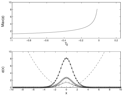
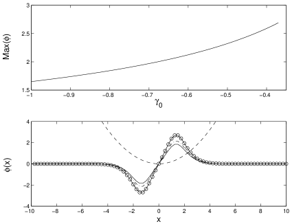
FIG. 1.: Bright solitons (left) and twisted solitons (right) obtained from Eq. (17) with $\gamma_{0}<0$, $\gamma_{1}=0.5$, $\Omega^{2}=0.4$, and $\omega=0.5$. The top subplot shows the solution maximum for different values of $\gamma_{0}$. The bottom subplot shows the potential (dashed line) and the solutions: at the left panel the solution is shown for $\gamma_{0}=-0.8$ (solid), $-0.6$ (dash-dotted), $-0.4$ (dotted) $-0.2$ (circles) and $-0.02$ (stars) and at the right panel for $\gamma_{0}=-0.8$ (solid), $-0.6$ (dash-dotted) and $-0.37$ where the branch ceases to exist (circles).

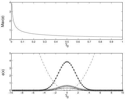
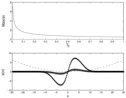
FIG. 2.: Similar to the first figure but for Thomas-Fermi clouds (left) and dark solitons (right) obtained from Eq. (17) with $\gamma_{0}>0$, $\gamma_{1}=0.5$, $\omega=0.5$, while $\Omega^{2}=0.4$ (left) and $\Omega^{2}=0.02$ (right). The top subplot shows the solution maximum for different values of $\gamma_{0}$. The bottom subplot shows the potential (dashed line) and the solutions for $\gamma_{0}=0.8$ (solid) , $0.6$ (dash-dotted), $0.4$ (dotted), $0.2$ (circles) and $0.01$ (stars). Notice that in the case of the dark soliton in the right subplot, the solution profile is altered very slightly between the cases $\gamma_{0}=0.8$ and $\gamma_{0}=0.2$, which are practically indistinguishable.

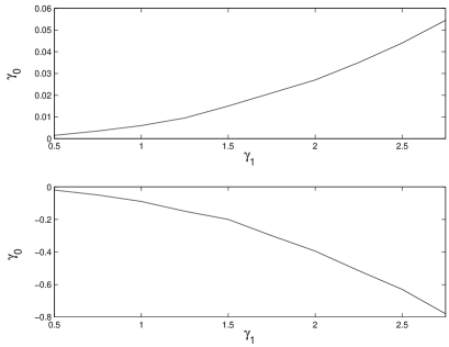
FIG. 3.: Domain of existence of dark (top panel for $\Omega^{2}=0.02$) and bright (bottom panel for $\Omega^{2}=0.4$) solitons of Eq. (17) with $|\omega|=0.5$. The solutions exist above and below, respectively, the corresponding curves of the ($\gamma_{0},\gamma_{1}$) plane.

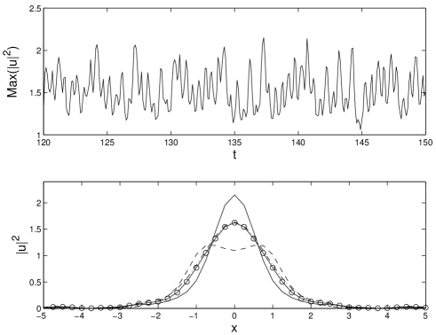
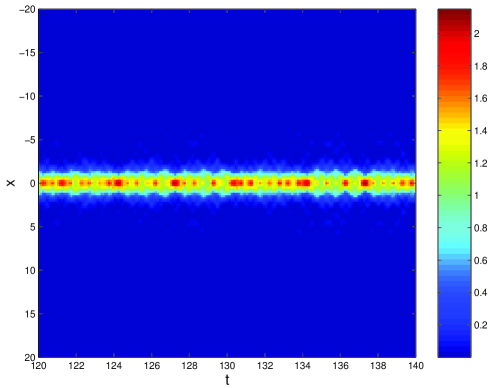
FIG. 4.: Temporal evolution of the bright soliton with $\gamma_{0}=-0.5$, $\gamma_{1}=1$, $\Omega^{2}=0.4$, and $\omega=0.5$. The top panel shows evolution of the (spatial) maximum of $|u|^{2}(x,t)$ as a function of time. The middle panel shows the solution $|u|^{2}(x,t)$ at $t=137.3$ (solid) and $t=138$ (dashed), their average (circles), and the initial configuration (dash-dotted). The latter practically coincides with the average. The bottom panel shows a contour plot of $|u|^{2}(x,t)$ in $(x,t)$.

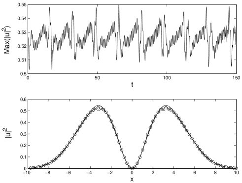
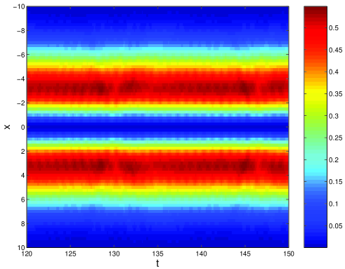
FIG. 5.: Same as Fig. 4, but for the dark soliton with $\gamma_{0}=0.5$, $\gamma_{1}=1$, $\Omega^{2}=0.02$, and $\omega=-0.5$. The maximum and minimum snapshots correspond to $t=128.4$ and $t=130.2$. The dash-dotted line of the theoretical prediction (initial condition) again coincides with the average denoted by the circles.

REFERENCES

- [1] C. Sulem and P.L. Sulem, The Nonlinear Schrödinger Equation, Springer-Verlag (New York, 1999).
- [2] For a recent survey of optical applications see Yu.S. Kivshar and G.P. Agrawal, Optical Solitons From Fibers to Photonic Crystals, Academic Press (2003).
- [3] For a recent survey of atomic physics applications see F. Dalfovo et al., Rev. Mod. Phys. 71, 463 (1999).
- [4] For a recent survey of dispersion management, see S.K. Turitsyn et al, C.R. Physique 4, 145 (2003).
- [5] I. Gabitov and S. Turitsyn, Opt. Lett. 21, 327 (1996); I. Gabitov and S. Turitsyn, JETP Lett. 63, 814 (1996); M.J. Ablowitz and G. Biondini, Opt. Lett. 23, 1668 (1998).
- [6] D.E. Pelinovsky and V. Zharnitsky, SIAM J. Appl. Math. 63, 745 (2003).
- [7] T.S. Yang and W.L. Kath, Opt. Lett. 22, 985 (1997); T.I. Lakoba and D.E. Pelinovsky, Chaos 10, 539 (2000).
- [8] I. Towers and B.A. Malomed, J. Opt. Soc. Am. 19, 537 (2002); L. Bergé et al., Opt. Lett. 25, 1037 (2000).
- [9] S. Inouye et al., Nature 392, 151 (1998); J. Stenger et al., Phys. Rev. Lett. 82, 2422 (1999); J.L. Roberts et al., Phys. Rev. Lett. 81, 5109 (1998); S.L. Cornish et al., Phys. Rev. Lett. 85, 1795 (2000); E.A. Donley et al., Nature 412, 295 (2001).
- [10] P.G. Kevrekidis et al., Phys. Rev. Lett. 90, 230401 (2003).
- [11] F.Kh. Abdullaev et al., Phys. Rev. Lett. 90, 230402 (2003); F.Kh. Abdullaev et al., Phys. Rev. A 67, 013605 (2003); F.Kh. Abdullaev et al., cond-mat/0306281.
- [12] H. Saito and M. Ueda, Phys. Rev. Lett. 90, 040403 (2003).
- [13] S. Burger et al., Phys. Rev. Lett. 83, 5198(1999); J. Denschlag et al., Science 287, 97 (2000); B. P. Anderson et al., Phys. Rev. Lett. 86, 2926 (2001); K.E. Strecker et al., Nature 417, 150 (2002); L. Khaykovich et al., Science 296, 1290 (2002).
- [14] V.M. Pérez-García, H. Michinel and H. Herrero, Phys. Rev. A 57, 3837 (1998); L. Salasnich, A. Parola and L. Reatto, Phys. Rev. A 65, 043614 (2002); Y.B. Band, I. Towers, and B.A. Malomed, Phys. Rev. A 67, 023602 (2003).
- [15] J.A. Sanders and F. Verhulst, Averaging Methods in Nonlinear Dynamical Systems, Springer-Verlag (Berlin, 1985).
- [16] P.G. Kevrekidis et al., New J. Phys. 5, 64 (2003).