Fluctuations impact on a pattern-forming model of population dynamics with non-local interactions

Abstract

A model of interacting random walkers is presented and shown to give rise to patterns consisting in periodic arrangements of fluctuating particle clusters. The model represents biological individuals that die or reproduce at rates depending on the number of neighbors within a given distance. We evaluate the importance of the discrete and fluctuating character of this particle model on the pattern forming process. To this end, a deterministic mean-field description, including a linear stability and a weakly nonlinear analysis, is given and compared with the particle model. The deterministic approach is shown to reproduce some of the features of the discrete description, in particular, the existence of a finite-wavelength instability. Stochasticity in the particle dynamics, however, has strong effects in other important aspects such as the parameter values at which pattern formation occurs, or the nature of the homogeneous phase.

1 Introduction

Pattern formation in the presence of fluctuations [1, 2] is a subject attracting much interest since the beginnings of instability studies. The most common way to model the process is in terms of stochastic field equations in which the deterministic part undergoes a pattern forming instability and a noise term modifies the dynamics. In situations where fluctuations are of internal origin, as for example arising from the discrete nature of the particles integrating the system, a more fundamental description is in terms of the microscopic particle dynamics (an analogy between a particular competing individual system with a reaction-diffusion system is presented in [3]). Models of interacting particle systems leading to periodic pattern formation are however not abundant in the literature. We introduced recently [4] one such a model, inspired in the interactions of biological individuals that compete for the resources around them and generalizing a model introduced in the context of plankton populations [5] . It consists in a set of random walkers, each one reproducing or dying with probabilities depending on the number of other individuals in a neighborhood. In our previous work [4] we presented a detailed numerical study of the model in two dimensions whose main result can be summarized in the existence of a stationary periodic pattern of clusters of particles for a specific range of parameters. A continuum Langevin equation is then derived under certain approximations for the density of particles, with a rather complicated noise term. A linear stability analysis is then performed on the deterministic (noiseless) equation that in two dimensions predicts the transition to periodic patters by a finite-wavelength instability. However, some numerical results, like the value of the parameters at which patterns emerge, are not well reproduced in the deterministic density equation. This reflects that the role of fluctuations (the noise term in the Langevin equation) maybe rather important depending on the properties of the system one wants to focus on.

In this context, we present in this Paper additional results for the model, with more emphasis on the one-dimensional case, and compare it more carefully with descriptions in which fluctuations are absent: a mean-field approximation and its amplitude equation. The onedimensional case is relevant by itself (see for example a relevant experimental situations in [6] and references therein), and also because it allows for a simpler analytical treatment. The amplitude equation in this work is calculated for both the one- and two-dimensional situations, but it is only the onedimensional expression which turns out to be suitable for full comparisons with the numerics. It is also worth mentioning some other extensions with respect to the results shown in [4]: the analytical results are stated for a general Kernel (see Sect. IV) of the mean-field density equation, and two order parameters are identified in the model, $\sqrt{I(0)}$ and $\sqrt{I(k_{m})}$, which inform, respectively, about the empty-active transition and the pattern formation transition (see Sect. III).

The Paper is organized as follows: In Sect. 2 we present the particle model, and show numerical results on its behavior in Sect. 3. Section 4 deals with the mean-field approximation, including its linear and weakly nonlinear analysis. We close with the Conclusions.

2 A model of nonlocally interacting individuals

We consider here both the one-dimensional situation ($d=1$), in which the system, consisting of $N(t)$ particles, is contained in a line, and the two-dimensional one ($d=2$), in which the $N(t)$ particles are in a square. In both cases we use periodic boundary conditions. At the starting time $t=0$ an initial population of $N(0)$ particles is randomly distributed. At time $t$, when the population is $N(t)$, one particle is selected at random (say particle $j$) and it dies (thus disappearing from the system) with probability $p_{j}$, reproduces (i.e. it replicates itself) with probability $q_{j}$, or is left unchanged with probability $1-p_{j}-q_{j}$. In the case of reproduction the newborn is placed at the same location as the parent particle. The process is repeated $N(t)$ times. After this, each particle moves independently in a random direction for a distance drawn from a Gaussian distribution of standard deviation $\sigma$, then time is incremented an amount $\tau$ ($t\rightarrow t+\tau$), and the algorithm repeats with the resulting $N(t+\tau)$ individuals. The random motion leads to diffusion with a diffusion coefficient $D=\sigma^{2}/2\tau$. The key point is the election of the probabilities $p_{j}$ and $q_{j}$ or, equivalently, the death and reproduction rates $\beta_{j}=p_{j}/\tau$ and $\lambda_{j}=q_{j}/\tau$, respectively. We choose a constant death rate $\beta_{j}=\beta_{0}$, $\forall j$, but the reproduction rate of particle $j$ depends of the number of particles $N_{R}^{j}$ within a distance $R$ from its position:

$$\lambda_{j}=\left\{\begin{array}[]{cl}\lambda_{0}-gN_{R}^{j}&\mbox{if}\ \ N_{R}^{j}\leq\lambda_{0}/g\\ 0&\mbox{if}\ \ N_{R}^{j}\geq\lambda_{0}/g\end{array}\right.$$ (3)

This kind of interaction models a slowing down of birth rates (until total suppression) in regions of high particle density. This is rather appropriate to model biological populations that compete for food or other resources present in a neighborhood of their positions, or that release toxic chemicals.

We choose $\lambda_{0}+\beta_{0}=1/\tau$, and introduce the maximum net growth rate $\mu\equiv\lambda_{0}-\beta_{0}$. For fixed $\tau$, the value of $\mu$ fixes both $\lambda_{0}$ and $\beta_{0}$. Since $p_{j}$ and $q_{j}$ are probabilities, we see that $\mu\tau\in[-1,1]$. One can estimate an equilibrium average density in this model by imposing that at each site birth and death compensate on average: $\lambda_{0}-g\langle N_{R}^{j}\rangle=\beta_{0}$. By assuming a uniform average density, $\phi$, one can express the number of neighbors as $\langle N_{R}^{j}\rangle=\phi hR^{d}$ ($h$ is $2$ in one dimension and $\pi$ in two dimensions, so that $hR^{d}$ is the length or the area of the neighborhood of a particle; we have not discounted the central particle from the number $N_{R}^{j}$, since a difference of one particle is irrelevant in the regime this argument is intended to describe). Thus

$$\phi\approx\frac{\mu}{ghR^{d}}\ .$$ (4)

But this estimation completely neglects inhomogeneities and diffusion. Fluctuations are known to produce inhomogeneities that alter estimations such as (4). This is specially true in situations like this where, in addition to (4), there is another homogeneous state where birth and death processes also compensate: the empty state $\phi=0$ ($N(t)=0$), for which both rates vanish. This is an absorbing state [7] since further evolution is impossible if the system reaches it. A phase transition to the absorbing state is expected by reducing the net growth rate $\mu$ from a higher value. The character of the transition and the location of the transition point are not well reproduced if fluctuations are neglected [7, 8].

3 Numerical observations

We first consider the one-dimensional case. The particle model described above is run on a ring of length $L=1$. For $\mu$ smaller than a critical value $\mu_{0}$, all initial particle distributions that we have checked end up attracted by the absorbing empty state. An illustrative way of showing one-dimensional particle dynamics consists in plotting the particle positions in the horizontal axis and the time evolution of these in the vertical. Proceeding in this way, Fig. 1 shows an example of the dynamics of the emptying process, strongly reminiscent of directed percolation [8] below threshold.

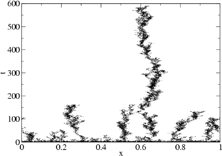
Figure 1: Time evolution (in vertical) of the particle positions (in horizontal) for $\mu=0.4$, $D=10^{-5}$, $R=0.1$, and $g=1/50$, starting from an initial population of 1000 particles. Units of time are such that $\tau=1$, and system size is $L=1$. The final state is empty of particles

By increasing the net growth, $\mu$, two situations appear: If the diffusion coefficient is large enough, an active phase, roughly homogeneous as shown in Fig. 2, appears above a critical value $\mu_{0}$. The value of $\mu_{0}$ is larger than the one required to equilibrate maximum birth rate and deaths ($\mu=0$). Moreover the average density is smaller than the predicted by the crude estimation (4).

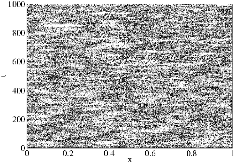
Figure 2: Idem as in Fig. (1) except for $\mu=0.46$ and $D=3\cdot 10^{-4}$. An active homogeneous phase has developed.

The other situation appears for smaller diffusion coefficients: now increasing $\mu$ above $\mu_{0}>0$ particles organize in clusters which are roughly equidistant, so that a periodic pattern results (Figs. 3 and 4). The configurations are rather noisy, specially close to the transition (Fig. 3), but a periodicity in the pattern is clear.

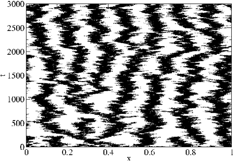
Figure 3: Idem as in Fig. (1) except for $\mu=0.50$. Noisy pattern formation has occurred.

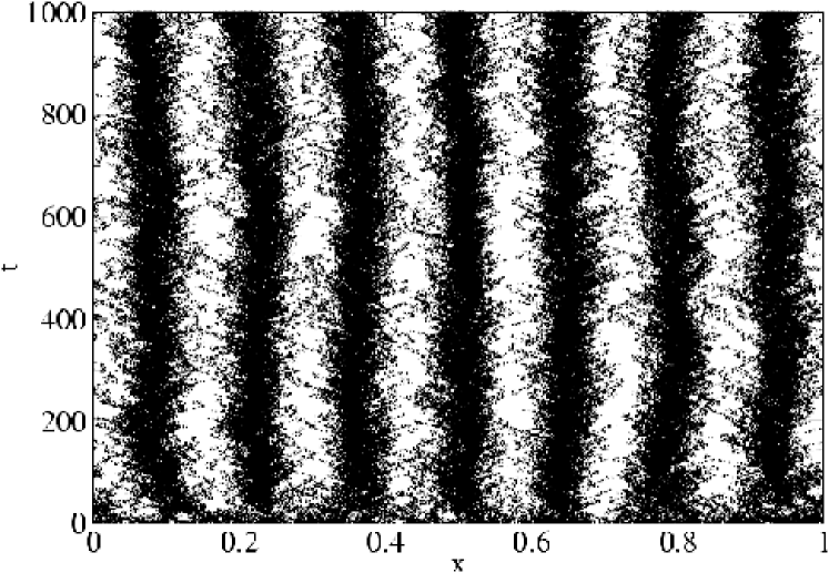
Figure 4: Idem as in Fig. (1) except for $\mu=0.90$. A rather well defined pattern is reached soon.

In the two-dimensional case the general scenario is similar, and was already described in [4]. Patterns consist in fluctuating particle clusters arranged in a hexagonal lattice. We show a snapshot in Figure 5.

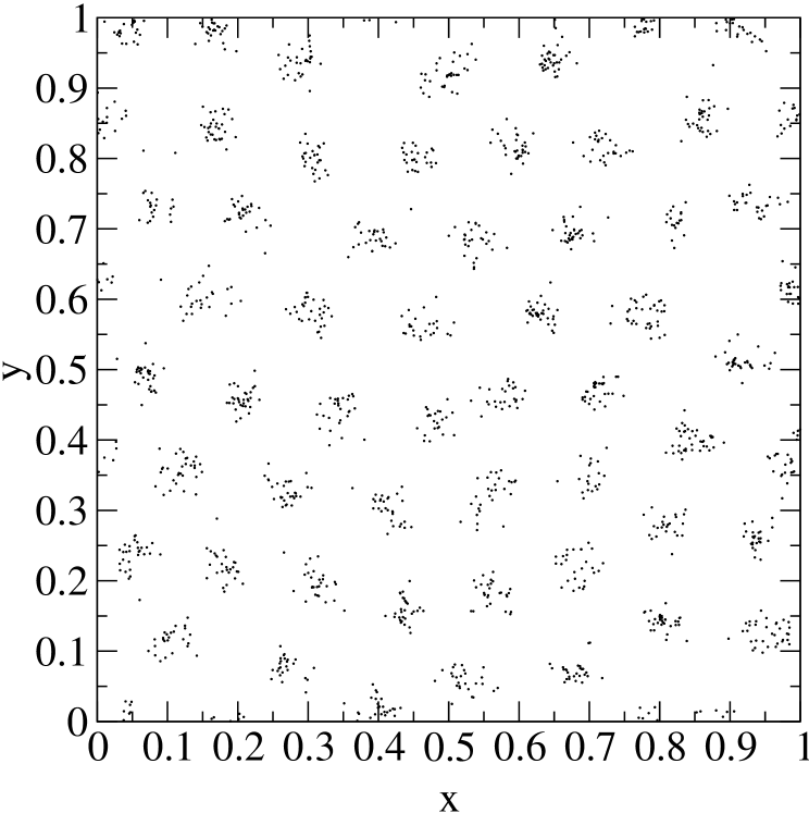
Figure 5: A snapshot of the fluctuating two-dimensional pattern of particle clusters, obtained in a square of side $L=1$ for $\mu=0.7$, $D=10^{-5}$, $R=0.1$, $g=1/50$, and $\tau=1$.

In order to be more quantitative, we introduce a structure function

$$I(k)=\left<\left|\sum_{j=1}^{N(t)}e^{i{\bf k}\cdot{\bf x}_{j}}\right|^{2}\right>\ .$$ (5)

The sum is over particles, at positions ${\bf x}_{j}$, and the average is a temporal average on a long-time state, performed to improve statistics. Maxima in $I(k)$ identify the wavenumbers, $k=|{\bf k}|$, associated to periodicities in the system. In any nonempty state there is also a peak in $k=0$ giving the square of the mean particle density. The values $I(0)$ and $I(k_{M})$, where $k_{M}$ is the nonvanishing wavenumber at which there is a maximum, act as two order parameters: the first one for the transition from the empty to the active phase, and the second for the pattern formation. For Figs. 3 and 4, $k_{M}=14\pi$, corresponding to the observation that the pattern consists of $7$ cells (a pattern of $n$ cells is characterized by a wavenumber $k_{M}=2\pi n/L$). In Fig. 6 we plot the value of $\sqrt{I(0)}$ and $\sqrt{I(k_{M})}$ as a function of $\mu$ in a different case for which $k_{M}=10\pi$ (i.e. 5 cells). Both order parameters become nonvanishing at the same absorbing transition, although with rather different amplitudes and behavior.

Figure 6: Values of $\sqrt{I(0)}$ (squares) and $\sqrt{I(k_{M})}$ (circles) as a function of $\mu$ for the one-dimensional particle model at $D=9.2\cdot 10^{-5}$, $R=0.13$, $g=1/120$, $\tau=1$ and $L=1$, for which $k_{M}=10\pi$. The upper thick line is $\phi_{s}$, from (36), and the lower one is $\phi_{p}$, from (37).

4 Mean-field description

We try now to understand the pattern forming processes described in the previous Section. It is obvious that the patterns are rather noisy, suggesting that fluctuations play a rôle in its development. It is known from related models [9, 5, 10] that, in addition to its impact on the absorbing transition, reproductive fluctuations have another important effect arising from the asymmetry between birth and death: Birth is a multiplicative process that increments the density in regions where it is already high, whereas death can occur anywhere. Thus, even if the average rates are equal, under reproductive fluctuations there is a tendency of the particles to organize into clusters of high density, leading to very inhomogeneous configurations when diffusion is not strong and is the only homogenizing force [9, 5, 10]. This inhomogeneity is amplified when birth rate exceeds death, but it is not observed in the common situations in which the growth is saturated by local interactions [8]. Thus, it is not obvious whether the pattern development in our model arises from the stochastic microscopic fluctuations, or if rather it is caused by some deterministic instability arising from the nonlocal interactions.

To address this question we can write down a mean-field-like description of the model, which completely neglects fluctuations, and check if the instability is present there. The mean-field equation is written in terms of an expected density $\phi({\bf x},t)$ as follows

$$\partial_{t}\phi({\bf x},t)=\mu\phi({\bf x},t)+D\nabla^{2}\phi({\bf x},t)-g\phi({\bf x},t)\int_{S}G({\bf x}-{\bf y})\phi({\bf y},t)d{\bf y}\ .$$ (6)

The first and second terms are the standard mean-field description of the net growth and the diffusion processes. The last one is a nonlocal contribution associated to the saturation produced by the neighborhood interactions in our model if the kernel $G({\bf x})$ is given by

$$G({\bf x})=\left\{\begin{array}[]{cl}1&\mbox{if}\ \ |{\bf x}|\leq R\\ 0&\mbox{if}\ \ |{\bf x}|\geq R.\end{array}\right.$$ (9)

$S$ is the domain were the system is defined. Equation (6) was more systematically deduced in [4] from our microscopic model, as the deterministic part of a Langevin equation containing rather complex noise terms. Equation (6) and related ones have also been proposed independently to model directly the macroscopic behavior of a variety of biological systems [11, 12, 13, 14]. In these cases, other kernels were considered in addition to (9), and for some of them pattern formation was observed. In the following we establish properties of (6) for general interaction kernels such that $G=G(|{\bf x}|)$, although the final results will be only commented for the step kernel given by (9). We first establish general relationships, then perform a linear stability analysis of a homogeneous solution, and then consider the weakly nonlinear behavior. We restrict to domains $S$ either unbounded or with periodic boundary conditions.

4.1 General relationships and homogeneous solutions

It is useful to write Eq. (6) in non-dimensional form to have a clearer idea of the independent parameters involved. We rescale the units of space, time, and $\phi$ as follows:

$${\bf u}=\frac{{\bf x}}{R}\ ,\ \ \ s=\frac{t}{R^{2}/D}\ ,\ \ \ \Psi({\bf u},s)=\frac{\phi({\bf x},t)}{D/gR^{2+d}}\ .$$ (10)

In this way:

$$\partial_{t}\Psi({\bf u},s)=\tilde{\mu}\Psi({\bf u},t)+\nabla_{u}^{2}\Psi({\bf u},t)-\Psi({\bf u},t)\int_{E}H({\bf u}-{\bf v})\Psi({\bf u},t)d{\bf y}\ .$$ (11)

$E$ is the rescaled domain, and $H({\bf u})$ is the rescaled kernel: $H({\bf u})=G({\bf x}=R{\bf u})$. In this mean-field description, The only relevant parameter turns out to be

$$\tilde{\mu}\equiv\frac{\mu R^{2}}{D}\ .$$ (12)

For future reference we introduce

$$\hat{H}(q)=\int_{E}H({\bf u})e^{i{\bf q}\cdot{\bf u}}d{\bf u}\ ,$$ (13)

and the notation $h\equiv\hat{H}(0)=\int_{E}H({\bf u})d{\bf u}$. Because of the symmetry assumed for $G({\bf x})$, $\hat{H}(q)$ depends only on the modulus of the wavenumber $q=|{\bf q}|$. For our step kernel we have, in the one-dimensional case:

$$\hat{H}(q)=2\frac{\sin(q)}{q}\ ,\ \ \ h=2$$ (14)

and for the two-dimensional case

$$\hat{H}(q)=2\pi\frac{J_{1}(q)}{q}\ ,\ \ \ h=\pi\ .$$ (15)

$J_{1}(q)$ is the first order Bessel function.

The trivial solution $\Psi$=$0$ of (11) becomes unstable for $\tilde{\mu}>0$. Then a uniform solution appears:

$$\Psi({\bf u},t)=\frac{\tilde{\mu}}{h}\equiv\nu\ ,$$ (16)

corresponding to

$$\phi({\bf x},t)=\frac{\mu}{ghR^{d}}\equiv\phi_{s}\ .$$ (17)

This reproduces the crude approximation (4), performed for the particle model. It is convenient to introduce the deviation $\psi$ with respect to the homogeneous solution:

$$\Psi({\bf u},t)=\frac{\tilde{\mu}}{h}+\psi({\bf u},t)\ ,$$ (18)

so that (11) reads

$$\partial_{t}\psi({\bf u},t) = \nabla_{u}^{2}\psi({\bf u},t)$$ (19)

$$- \nu\int_{E}H({\bf u}-{\bf v})\psi({\bf v},t)d{\bf v}-\psi({\bf u},t)\int_{E}H({\bf u}-{\bf v})\psi({\bf v},t)d{\bf v}\ .$$

4.2 Linear stability analysis

The linear stability analysis of the homogeneous solution can now readily performed by introducing perturbations of the form $\psi\approx\exp(i{\bf q}\cdot{\bf u}+\lambda(k)t)$ and neglecting nonlinear terms. The perturbation growth rate is

$$\lambda(q)=-q^{2}-\nu\hat{H}(q)\ .$$ (20)

It is seen that a necessary condition for instability is that $\hat{H}(q)$ takes negative values (note that Eq. (20) generalizes to an arbitrary kernel the expression shown in [4] for the step kernel) . It is also sufficient, since instability will always be reached in this case by increasing sufficiently $\nu$ (or $\tilde{\mu}$). Thus, if $\hat{H}(q)<0$ for some range of $q$, there is a critical value of $\nu$, $\nu_{c}$ (corresponding to a critical $\tilde{\mu}_{c}$) such that an instability to pattern formation occurs [12, 4]. Since both (14) and (15) take negative values, we see that the mean-field model with the step kernel undergoes a pattern forming instability without the need of any stochastic noise, as already reported [11, 4, 12]. Figure 7 (left) plots expression (20) in the one-dimensional case, showing the change of sign of $\lambda(q)$ around a critical $q_{c}$ by increasing $\tilde{\mu}=\nu h$. Figure 8 (left) shows a long-time numerical solution of (6)-(9) in one dimension, displaying a well-developed steady pattern. The right part of Fig. 8 shows the analogous structure in two dimensions: the instability leads to the formation of a pattern of hexagonal symmetry, as in the particle model. The corresponding two-dimensional dispersion relation (20) is shown in the right part of Fig. 7.

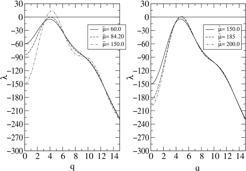
Figure 7: The linear growth rate (20) of perturbations of wavenumber $q$ to the homogeneous solution (16). Left: $d=1$. Right: $d=2$. In both cases positive growth, i.e. instability, arises by increasing $\tilde{\mu}$.

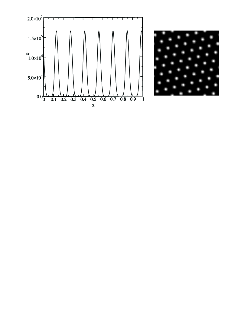
Figure 8: Steady periodic patterns obtained by long-time integration of the mean-field model (6) in $d=1$ (left) and $d=2$ (right). In both cases $\mu=0.7$, $D=10^{-5}$, $R=1$, and $g=1/50$. In the second case higher values of $\phi$ are represented by lighter gray levels.

Eq. (20) explains also the absence of instability for other kinds of kernels, such as the Gaussian one, for which $\hat{H}(q)$ is positive definite [13, 11, 12] (we stress however that patterns may appear under front propagation, or in response to spatial inhomogeneities [13]). To make a more quantitative analysis, the value of $\nu_{c}$ and the fastest growing wavenumber $q_{c}$ are obtained from the simultaneous solution of

$$q_{c}^{2}+\nu_{c}\hat{H}(q_{c}) = 0$$

$$2q_{c}+\nu_{c}\hat{H}^{\prime}(q_{c}) = 0\ .$$ (21)

Numerical solution of these equations leads, for the one-dimensional case and step kernel:

$$q_{c}\approx 4.078\ ,\ \ \ \nu_{c}\approx 42.10\ ,$$ (22)

so that $\tilde{\mu}_{c}\approx 84.20$. In two dimensions:

$$q_{c}\approx 4.779\ ,\ \ \ \nu_{c}\approx 58.948\ ,$$ (23)

and $\tilde{\mu}_{c}\approx 185.192$. From (10), the unscaled values ${\bf k}$ of the wavenumbers are given by ${\bf k}={\bf q}/R$.

These predictions can be compared with the numerical observations of the particle model. First, the maximum of the structure function for the patterns in the Figs. 3 and 4 was at $k=14\pi\approx 43.98$. This is precisely the first wavenumber compatible with the periodic boundary conditions immediately above the fastest growing mode in the mean-field equation for $R=0.1$: $k_{c}=q_{c}/R\approx 40.78$. For the configurations of periodic character among the ones used to construct Fig. 6, the maximum in the structure function was at $k=10\pi\approx 31.4159$, to be compared with $k_{c}=q_{c}/R\approx 31.369$ for $R=0.13$. The agreement is thus excellent in both cases. We can conclude that the essential mechanism of the pattern forming instability is well captured by the deterministic description, being the period of the pattern even quantitatively reproduced. For the two-dimensional case, the same agreement was already observed [4].

The situation is different for the location of the point of pattern onset. As for the location of the absorbing transition, the mean-field prediction and the particle model disagree. Typically, the transition from the empty state to the pattern is observed directly, without the intermediate of the homogeneous distribution. Only if diffusion is greatly increased the homogeneous state is observed (Fig. 2) but then the transition to patterns predicted by (22) occurs at $\mu$ exceeding the maximum of the physical range $\mu\tau\in[-1,1]$ (and it is indeed not observed in the particle model, which is a kind of agreement). The reason for this disagreement, despite containing the correct instability mechanism, is easy to understand: In cases such as the ones in Sect. 3 with small $D$ ($D=10^{-5}$) it happens that the predicted value of $\mu_{c}$ ($=0.084$) is much smaller than the $\mu_{0}$ of the absorbing transition (which is $\approx 0.45$). Thus it is not strange than, as soon as the active phase becomes preferred above $\mu_{0}$, it is already of the periodic type. The failures of the mean-field approach to fully describe the pattern behavior are then due to the strong impact of microscopic fluctuations on the absorbing transition. A second case is the one corresponding to Fig. 6. Here $\mu_{c}=0.458>\mu_{0}\approx 0.3$. But what is observed is that, even when the system is below threshold, microscopic fluctuations excite the less-damped modes [1, 2], so that a small amplitude noisy pattern is always present above the absorbing transition, as seen in Fig. 6. Fluctuation strength is relatively large here because of the low amplitude of the active state close to $\mu_{c}$, caused by the proximity to $\mu_{0}$. Pattern formation is not a sharp bifurcation in this case, but a continuous crossover. Finally, in the situation in which the absorbing transition and the pattern forming instability would be well separated, this last one falls outside the physical range $\mu\tau\in[-1,1]$.

4.3 Weakly nonlinear amplitude equations

The advantage of having a continuum model as (6) is the possibility to use the tools of pattern formation theory [15, 16] to obtain analytic results. A first example has been the linear stability analysis performed before. We now estimate the pattern amplitude close to threshold by calculating the pertinent amplitude equations.

To this end we start from Eq. (19), and perform the standard expansions in a small parameter $\epsilon$ related to the distance to threshold:

$$\psi({\bf x},t)=\epsilon\psi_{1}({\bf u},T_{1},T_{2},...)+\epsilon^{2}\psi_{2}({\bf u},t,T_{1},T_{2},...)+\epsilon^{3}\psi_{3}(x{\bf u},t,T_{1},T_{2},...)+...$$ (24)

$$\nu=\nu_{c}+\epsilon\nu_{1}+\epsilon^{2}\nu_{2}+...$$ (25)

We have introduced two slow time scales: $T_{1}=\epsilon t$, $T_{2}=\epsilon^{2}t$. For simplicity we do not introduce additional space variables, needed when considering large-scale pattern modulations.

To first order in $\epsilon$, one finds the equation

$$L_{c}\psi_{1}({\bf u},T_{1},T_{2})=0\ ,\ \ {\rm with}\ \ L_{c}=\partial_{t}-\nabla_{u}^{2}+\nu_{c}{\mathcal{H}}\ \ .$$ (26)

${\mathcal{H}}$ is the integral operator acting as ${\mathcal{H}}f({\bf u})\equiv\int_{E}H({\bf u}-{\bf v})f({\bf v})d{\bf v}$. Eq. (26) implies that $\psi_{1}$ is a combination of periodic patterns of the critical periodicity $2\pi/q_{c}$:

$$\psi_{1}({\bf u},T_{1},T_{2})=\sum_{j}A_{j}(T_{1},T_{2})e^{i{\bf q}_{j}\cdot{\bf u}}\ ,$$ (27)

with $|{\bf q}_{j}|=q_{c}$.

At orders $\epsilon^{2}$ and $\epsilon^{3}$ we find

$$L_{c}\psi_{2} = -\partial_{T_{1}}\psi_{1}-\nu_{1}{\mathcal{H}}\psi_{1}-\psi_{1}{\mathcal{H}}\psi_{1}$$ (28)

$$L_{c}\psi_{2} = -\partial_{T_{1}}\psi_{2}-\partial_{T_{2}}\psi_{1}-\nu_{1}{\mathcal{H}}\psi_{2}-\nu_{2}{\mathcal{H}}\psi_{1}-\psi_{2}{\mathcal{H}}\psi_{1}-\psi_{1}{\mathcal{H}}\psi_{2}\ \ .$$ (29)

We particularize to the one-dimensional case, in which the only possible planform of the form (27) is

$$\psi_{1}(u,T_{1},T_{2})=A(T_{1},T_{2})e^{iq_{c}u}+A^{*}(T_{1},T_{2})e^{-iq_{c}u}\ .$$ (30)

$A^{*}$ is the complex conjugate of $A$. Substituting in (28) one finds, as usual in one-dimensional patterns, that boundedness of the solutions implies $\nu_{1}=0$, so that $\epsilon\propto(\nu-\nu_{c})^{1/2}$ and $A(T_{1},T_{2})=A(T_{2})$. By solving (28) and substituting in (29), one finds the condition to avoid resonant terms:

$$\partial_{T_{2}}A=-\nu_{2}\hat{H}(q_{c})A-\kappa|A|^{2}A\ ,$$ (31)

which is the desired amplitude equation. Here,

$$\kappa = \hat{H}(q_{c})(Q+S)+\hat{H}(2q_{c})Q+\hat{H}(0)S$$

$$Q = \frac{-\hat{H}(q_{c})}{4q_{c}^{2}+\nu_{c}\hat{H}(2q_{c})}\ \ \ ,\ \ S=\frac{-2\hat{H}(q_{c})}{\nu_{c}\hat{H}(0)}$$ (32)

All these quantities are pure non-dimensional numbers. Their values, in addition to the ones given in (22), are $\hat{H}(0)=h=2$, $\hat{H}(q_{c})\approx-0.3950$, $\hat{H}(2q_{c})\approx 0.2341$, $Q=5.172\cdot 10^{-3}$, $S=9.383\cdot 10^{-3}$, and $\kappa=0.01423$. The content of (31) is more clearly seen by reintroducing the original time variable $t=\epsilon^{-2}T_{2}$ and the amplitude $B(t)=\epsilon A(T_{2})$ so that

$$\dot{B}(t)=(\nu-\nu_{c})\left(-\hat{H}(q_{c})\right)B-\kappa|B|^{2}B$$ (33)

The equation predicts that instability develops for $\nu>\nu_{c}$ and leads to a pattern of arbitrary phase, and amplitude

$$|B|=\sqrt{(\nu-\nu_{c})\frac{-\hat{H}(q_{c})}{\kappa}}$$ (34)

that has bifurcated supercritically from the homogeneous solution (16). Returning back to dimensional variables via (10), the periodic steady solution for the original density can be reconstructed as

$$\phi(x,t)=\phi_{s}+\phi_{p}\left(e^{i(k_{c}x+\varphi)}+e^{-i(k_{c}x+\varphi)}\right)+{\mathcal{O}}(\mu-\mu_{c})\ .$$ (35)

with

$$\phi_{s}=\frac{\mu}{2gR}$$ (36)

and

$$\phi_{p}=\sqrt{\mu-\mu_{c}}\ \frac{D^{\frac{1}{2}}}{gR^{2}}\ \sqrt{\frac{\hat{H}(q_{c})}{2\kappa}}\ .$$ (37)

$\varphi$ is an arbitrary phase. We can compare this analytic prediction with the particle patterns. The structure function (5) can be interpreted as the power spectrum of a density of the form $\sum_{i=1}^{N(t)}\delta({\bf x}-{\bf x}_{i})$. Comparing with the power spectrum of the mean-field density (35), we see that $\sqrt{I(0)}$ should be related to $\phi_{s}$, and $\sqrt{I(k_{M})}$ to $\phi_{P}$. We remind that $k_{M}$ was well reproduced by the mean-field value of $k_{c}$. Comparison is performed in Fig. 6. We see that the agreement in the amplitudes is poor (even if it was expected to be valid only close to $\mu_{c}$) although some of the trends are reproduced. The disagreement is linked to the failure to capture the correct transition points.

The amplitude equation can also be calculated in $d=2$, by using an hexagonal planform [15, 16] instead of (30):

$$\psi_{1}({\bf u},T_{1},T_{2})=\sum_{j=1,2,3}A_{j}(T_{1},T_{2})e^{i{\bf q}_{j}\cdot u}+{\rm c.c.}$$ (38)

${\bf q}_{j}$ ($j=1,2,3$), are three wavenumbers of modulus $q_{c}$ at $120$ degrees from each other, and c.c. means complex conjugate. The problem with such calculation is that generically the bifurcation to hexagons is subcritical, so that there is no guarantee that the amplitude equation will capture the saturation that occurs far from the instability point. By using (28)-(29) one finds,

$$\dot{B}_{1}(t)=(\nu-\nu_{c})\left(-\hat{H}(q_{c})\right)B_{1}+2\left(-\hat{H}(q_{c})\right)B_{2}^{*}B_{3}+{\mathcal{O}}(|B_{j}|^{2}B_{1})\ ,$$ (39)

and two other equations obtained by permuting cyclicly the indices $1,2,3$. As in (33), $B_{i}$ is the coefficient of the Fourier mode of wavenumber ${\bf q}_{i}$ in the expansion of $\psi({\bf x},t)$. Eq. (15) should be used for $\hat{H}(q_{c})$. The sign of the third order terms not written explicitly in (39) is such that they do not saturate the pattern. Thus, expansion should be followed at higher orders and (39) is of not much utility. Nevertheless, the presence of the second order term confirms that the bifurcation in the mean-field model is subcritical, and the positive sign of its coefficient (remember that $\hat{H}(q_{c})<0$) implies that the bifurcating solution leads to H0 or positive hexagons [16] (i.e. points of high density forming an hexagonal lattice), as observed in the particle model.

5 Conclusion

In this work we have presented new results on a model recently introduced by the authors [4] which considers particles reproducing and dying at rates depending on the number of individuals that every particle has in its $R$-ranged neighborhood. The study has been performed at the level of the density equation derived for this model, and mainly for the one-dimensional case, since analytical results are simpler here.

As the general conclusion of the comparison between the particle and the mean-field model we can say that, although the instability appears to be deterministic in origin and the mean-field approach captures correctly the wavenumber, fluctuations are important and affect transition points and amplitudes. This limits the usefulness of standard pattern forming theory tools, usually developed for continuum models as in the case of weakly nonlinear analysis, and ask for further studies in which noise terms are explicitly considered [4]. Fluctuations may have also another interesting effect: even in cases in which there is no deterministic instability, as for example when a Gaussian kernel is used in (6) [13, 11, 12], it is very likely that a corresponding particle model would display a small amplitude noisy pattern, arising by the less-damped models excited by fluctuations.

References

- [1] J.M. Sancho, J. García Ojalvo, Noise in Spatially Extended Systems (Springer, Berlin, 1999).
- [2] M. San Miguel, R. Toral in Instabilities and Nonequilibrium Structures VI, E. Tirapegui, J. Martínez, and R. Tiemann, Eds. (Kluwer Academic Publishers, 1999).
- [3] F. Bagnoli, M. Bezzi, Phys. Rev. Lett. 79 (1997) 3302.
- [4] E. Hernández-García and C. López, Clustering, advection and patterns in a model of population dynamics with neighborhood-dependent rates, e-print cond-mat/0310384, to appear in Phys. Rev. E (2004).
- [5] W.R. Young, A.J. Roberts, G. Stuhne, Nature 412, 328 (2001); W.R. Young in From stirring to mixing in a stratified ocean, Proceedings of the 12th ’Aha Huliko’a Hawaiian Winter Workshop, University of Hawaii at Manoa (2001).
- [6] A. L. Lin, B. A. Mann, G. Torres-Oviedo, B. Lincoln, J. Kas, and H. L. Swinney, Localization and extinction of bacterial populations under inhomogeneous growth conditions, e-print q-bio.PE/0310032.
- [7] G. Grinstein, M.A. Muñoz, in Fourth Granada Lectures in Computational Physics, P.L. Garrido and J. Marro editors (Springer, Berlin, 1997).
- [8] H. Hinrichsen, Adv. Phys. 49 (2000) 815 .
- [9] Y-C. Zhang, M. Serva, M. Polikarpov, J. Stat. Phys. 58 (1990) 849.
- [10] R. Adler in Monte Carlo simulation in oceanography, Proceedings of the 10th ’Aha Huliko’a Hawaiian Winter Workshop, University of Hawaii at Manoa (1997).
- [11] M.A. Fuentes, M.N. Kuperman, V.M. Kenkre, Phys. Rev. Lett. 91 (2003) 158104.
- [12] M.A. Fuentes, M.N. Kuperman, V.M. Kenkre, Analytic considerations in the study of spatial patterns arising from nonlocal interaction effects in population dynamics, e-print nlin.PS/0311017.
- [13] A. Sasaki, J. Theor. Biol. 186 (1997) 415.
- [14] N.M. Shnerb, Pattern formation and nonlocal logistic growth, e-print cond-mat/0311230.
- [15] M. C. Cross and P. C. Hohenberg, Rev. Mod. Phys. 65 (1993) 851.
- [16] D. Walgraef, Spatio-Temporal Pattern Formation: With Examples from Physics, Chemistry, and Materials Science (Springer, Berlin, 1996).