Moments of the first passage time under external driving

Abstract

A general theory is derived for the moments of the first passage time of a one-dimensional Markov process in presence of a weak time-dependent forcing. The linear corrections to the moments can be expressed by quadratures of the potential and of the time-dependent probability density of the unperturbed system or equivalently by its Laplace transform. If none of the latter functions is known, the derived formulas may still be useful for specific cases including a slow driving or a driving with power at only small or large times. In the second part of the paper, explicite expressions for mean and variance of the first passage time are derived for the cases of a linear or a parabolic potential and an exponentially decaying driving force. The analytical results are found to be in excellent agreement with computer simulations of the respective first-passage processes. The particular examples furthermore demonstrate that already the effect of a simple exponential driving can be fairly involved implying a nontrivial nonmonotonous behavior of mean and variance as functions of the driving’s time scale.

I Introduction

One of the key results in the theory of stochastic processes are the quadrature expressions for the moments of the first passage time (FPT) in case of a one-dimensional Markov process PonAnd33 ; Sie51 . One of the assumptions made in the seminal papers by Pontryagin et al. PonAnd33 and Siegert Sie51 is the temporal homogeneity of the process: except for the driving Gaussian white noise the system is subject to a force without time dependence. In many instances this assumption does not hold and an extension of the classic theory to the case of a time-dependent force is desirable.
In the context of many noise-induced phenomena, for instance, the presence of an additional deterministic or stochastic perturbation is essential and its effect on the passage time statistics is of foremost interest. In case of resonant activation (RA) DoeGad92 ; BieAst93 ; PecHan94 ; Rei95 , the additional driving is a stochastic process with state-dependent amplitude. For the problems of stochastic resonance (SR) (see Ref. GamHan98 and references therein) and coherent stochastic resonance (CSR) FleHav88 ; MasRob95 ; GitWei95 ; Por97 the driving is commonly a deterministic periodic signal. The key feature of both RA and CSR is a minimum in the mean FPT or mean exit time attained at a finite “optimal” value of the forcing’s time scale (e.g. correlation time or driving period). Similarly, SR is realized if a time-scale matching condition between the forcing period and the FPT of the unperturbed system (an inverse Kramers rate) is met.
My own interest in the general problem originates in studies of stochastic neuron models involving an exponentially decaying time-dependent forcing. For these models, the FPT corresponds to the interspike intervals (ISIs) separating the neural discharges (action potentials or spikes) by means of which neurons transmit and process signals. The exponentially decaying perturbation in these models arises from slow ionic currents that are driven by the spiking activity of the neuron itself LinLon03b . An exponential perturbation is also obtained via a simple transformation of models with a decaying threshold; such models have been employed to reproduce the statistics of certain sensory neurons ChaLon00 ; ChaPak03 . In general, the effect of an exponentially decaying driving on the FPT statistics is poorly understood up to now in contrast to the frequently studied case of periodically forced stochastic neuron models (see e.g. Refs. Lon93 ; BulLow94 ; BulEls96 ; PleTan97 ; Lan97 ; PleGei01 ).
In order to study the change of the FPT statistics induced by a time-dependent driving, researchers have used two different analytical approaches. First, keeping the potential shape, the driving force as well as the boundary and initial conditions as simple as possible allows in some cases for an exact, in others for an approximate solution. This kind of approach was pursued in the late 1980’s FleHav88 ; BalVan88 ; Bez89 and during the 1990’s DoeGad92 ; BieAst93 ; BulLow94 ; GitWei95 ; Por97 (see also Ref. Red01 , ch. 4 for further examples); in most cases (piecewise) linear potentials and a periodic or dichotomous driving were considered. Later several researchers proposed semi-analytic procedures to solve these FPT problems Men92 ; KlikYao01 ; ChoFox02 . It should also be noted that there exists a considerable mathematical literature on the FPT problem with time-dependent deterministic forcing, most of which is devoted to specific simple cases that are exactly solvable by a transformation to a time-homogeneous system (see Refs. GutGon91 ; GutRom95 ; GutRic97 and further references cited in these papers).
The other analytical approach consists of a weak noise analysis of driven first-passage processes. Here the only assumption made about the potential is the existence of a metastable state. Refs. SmeDyk99 ; LehRei00 ; Shu00 ; TalLuc03 focused on the escape rate out of a metastable one-dimensional potential (the inverse mean first passage time for a quasi-equilibrium initial condition) in the small-noise limit and aimed thus at a generalization of the famous Kramers problem Kra40 ; HanTal90 for periodic SmeDyk99 ; LehRei00 ; TalLuc03 or stochastic PecHan94 ; Rei95 driving. Although both approaches led to significant progress, there are also many instances where one wishes to go beyond the limit set by assuming weak noise or piecewise linear potentials and where also higher moments and not only the mean FPT (or its inverse) may be of interest.
Here I give an extension of the classic concept due to Pontryagin PonAnd33 and Siegert Sie51 of calculating the FPT moments for a general potential to the case that includes a weak time-dependent driving. I focus on a deterministic driving function; the approach might be, however, also helpful in situations with an additional stochastic driving. I will use a perturbation calculation that requires a weak driving and will consider the first (linear) correction term for each moment. No restrictions apply with respect to the noise intensity or the time scale of the driving, although the range of validity of the theory, i.e. the question how “weak” the driving has to be, may also depend on these parameters. My most general result relates the linear corrections to each moment of the FPT to quadratures of the time-dependent probability density $P_{0}(x,t)$ of the unperturbed system or to quadratures of the Laplace transform of this function. An alternative formulation provides the corrections in terms of an infinite sum of quadratures of known functions. These results cannot be applied in the general case (arbitrary driving function and arbitrary potential shape), since $P_{0}(x,t)$ and/or its Fourier transform are not known for most potentials and the numerical evaluation of an infinite sum of quadratures is in general not feasible either. For many important cases, however, including a slow driving, a driving with power at only small times or a driving with power at only large times, the derived general formulas can be useful for the FPT problem in a potential of arbitrary shape. Furthermore, I will show that for two specific potential shapes (linear and parabolic) and an exponentially decaying driving force, the derived theory yields valid (and in part strikingly simple) results for the FPT’s mean and variance for arbitrary time scale of the driving (slow, moderate, or fast compared to the mean FPT of the unperturbed system). The explicite results derived for an exponential driving function can be applied to the neurobiological problems mentioned above; this will be done elsewhere. Since the exponential decay of drift parameters is frequently encountered in many situations, the results may be also helpful for the study of other physical systems.
This paper is organized as follows. Sec. II starts with an introduction of the problem and of the quantities of interest. Next I present an derivation of alternative quadrature formulas for the FPT moments in the time-homogeneous case. These quadratures are entirely equivalent to the classic formulas by Siegert Sie51 as shown in the appendix. The alternative approach will be the basis for the perturbation calculation of the time-inhomogeneous first-passage problem leading to the general relation between the corrections of the moments and the quadratures of the unperturbed probability density. In sec. III, I derive explicite results for a linear and a parabolic potential and an exponential driving force. These analytical results will be compared to simulations of the two systems in sec. IV. Here I will show that, remarkably, similar to the case of periodic driving, a nontrivial behavior of the FPT’s mean and variance with respect to the time scale of the driving (i.e. the decay rate of the exponential driving) is possible. The mechanisms for these “resonances” will be discussed. Sec. V summarizes the findings and discusses further applications and extensions of the theory.

II General Theory

II.1 Langevin and Fokker-Planck equations

Starting point of my consideration is the Langevin equation for a one-dimensional escape process given by a potential $U(x)$, a white-noise driving of intensity $D$, and an additional weak time-dependent forcing $\varepsilon s(t)$:

$$\dot{x}=-U^{\prime}(x)+\varepsilon s(t)+\sqrt{2D}\xi(t)$$ (1)

Without loss of generality I consider an initial value at zero ($x(0)=0$) and ask for the first-passage time to a point $x_{E}$ to the right of the origin ($x_{E}>0$). The only restriction for the potential is that I exclude potentials that allow for an escape toward minus infinity. Furthermore, I do not specify the forcing $s(t)$ but take for granted that its effect on the FPT statistics is weak by virtue of the small parameter $\varepsilon$.
Instead of using the Kolmogorov (backward) equation as it is commonly done in the treatment of FPT problems Sie51 ; Gar85 , I shall employ the Fokker-Planck (forward) equation (FPE) governing the probability density of $x$

$$\partial_{t}P(x,t)=\partial_{x}[(U^{\prime}(x)-\varepsilon s(t))P(x,t)+D\partial_{x}P(x,t)].$$ (2)

The FPT problem stated above determines the initial condition (at $t=0$ the variable $x$ is with certainty at $x=0$) and the boundary condition (absorbing boundary condition at $x=x_{E}$)

$$P(x,0) = \delta(x),$$ (3)

$$P(x_{E},t) = 0.$$ (4)

It is well known that there is a simple relation between the FPT density and a quantity derived from the probability density $P(x,t)$: the FPT density is given by the time-dependent probability current at the absorbing boundary (see, for instance, Ref. Hol76 )

$$\Phi(T) = J(x_{E},T)=-[(U^{\prime}(x)-\varepsilon s(T))P(x,T)+D\partial_{x}P(x,T)]|_{x=x_{E}}$$ (5)

$$= -D\partial_{x}P(x,T)|_{x=x_{E}}.$$

Provided $\Phi(t)$ is known, one can calculate the moments of the FPT by

$$\langle T^{n}(0\to x_{E})\rangle=\int\limits_{0}^{\infty}dT\;T^{n}\Phi(T)=-D\int\limits_{0}^{\infty}dT\;T^{n}\partial_{x}P(x,T)|_{x=x_{E}}.$$ (6)

For certain problems it may be desirable to know also the Laplace transform of $\Phi(T)$. This function can be expressed by the Laplace transform of the probability density $\tilde{p}(x,p)$ as follows

$$\rho(p)=\int\limits_{0}^{\infty}dt\;e^{-pt}\Phi(t)=-D\partial_{x}\tilde{p}(x,p)\Bigg{|}_{x=x_{E}}.$$ (7)

By means of the Laplace transform the moments can be calculated as follows

$$\langle T^{n}(0\to x_{E})\rangle=(-1)^{n}\frac{d^{(n)}}{dp^{n}}\rho(p)\Bigg{|}_{p=0}.$$ (8)

However, even in the absence of a time-dependent driving ($\varepsilon=0$), solving directly for one of the functions $P(x,t)$, $\Phi(T)$, or $\rho(p)$ is possible only in a few simple cases including constant and linear potential shapes. Nevertheless, for calculating the moments of the FPT we are not restricted to use eq. (6) or eq. (8). Remarkably if $\varepsilon=0$, the moments of the FPT can be calculated exactly for an arbitrary potential shape $U(x)$. The general formula for the $n$-th moment of the passage from a general initial point $x=a$ to an absorbing boundary at $x=b$ is given by Sie51

$$\langle T^{n}(a\to b)\rangle_{0}=\frac{n}{D}\int_{a}^{b}dye^{U(y)/D}\int_{-\infty}^{y}dxe^{-U(x)/D}\langle T^{n-1}(x\to b)\rangle_{0}$$ (9)

where the index “0” indicates that $\varepsilon=0$ (later on, this convention will be also applied to the functions $P(x,t),\tilde{p}(x,p)$ and $\rho(p)$). In order to calculate the $n$-th moment one has to solve for the lower moments as functions of the initial point first. The hierarchy of quadratures is completed by stating that for obvious reasons $\langle T^{0}(a\to b)\rangle=\langle 1\rangle=1$.
The aim of this paper is to extend these expressions to the case of a weak time-dependent driving function $\varepsilon s(t)$. In other words, I seek for the linear correction term to the n-th moment denoted $j_{n}(x_{E})$ such that

$$\langle T^{n}\rangle=\langle T^{n}\rangle_{0}+\varepsilon j_{n}(x_{E}).$$ (10)

In particular, once the corrections to the first two moments have been calculated, mean and variance of the FPT will be to linear order in $\varepsilon$ given by

$$\langle T\rangle = \langle T\rangle_{0}+\varepsilon j_{1}(x_{E}),$$ (11)

$$\langle\Delta T^{2}\rangle = \langle T^{2}\rangle-\langle T\rangle^{2}$$ (12)

$$= \langle\Delta T^{2}\rangle_{0}+\varepsilon[j_{2}(x_{E})-2\langle T\rangle_{0}j_{1}(x_{E})].$$

Later on, for specific systems, I will solely discuss these first two cumulants and the relative standard deviation (coefficient of variation) of the FPT, that is a function of them

$$CV=\frac{\sqrt{\langle\Delta T^{2}\rangle}}{\langle T\rangle}.$$ (13)

II.2 Moments of the first passage time in the autonomous case - the other way around

Here I set $\varepsilon=0$. First I introduce the functions

$$\beta_{n}(x)=\int_{0}^{\infty}dt\;\;t^{n}P(x,t)$$ (14)

and

$$J_{n}(x)=-(U^{\prime}(x)+D\frac{d}{dx})\beta_{n}(x)$$ (15)

On comparing eq. (6) and eqs. (14) and (15) it becomes apparent that $\beta_{n}$ and $J_{n}$ are related to the $n$-th moment of the FPT as follows

$$\langle T^{n}\rangle_{0}=-D\beta^{\prime}_{n}(x_{E})=J_{n}(x_{E}).$$ (16)

Here and in the following the prime denotes the derivative with respect to $x$. I now derive the general solutions for $J_{n}(x)$ that provides an alternative solution for the FPT moments by virtue of eq. (16).
Multiplying the FPE (2) with $t^{n}$, integrating over $t$, and using integration by part on the l.h.s. of the equation, I obtain for the functions $\beta_{n}(x)$ the following set of equations

$$-\delta(x) = \frac{d}{dx}(U^{\prime}(x)+D\frac{d}{dx})\beta_{0}(x),$$ (17)

$$-n\beta_{n-1}(x) = \frac{d}{dx}(U^{\prime}(x)+D\frac{d}{dx})\beta_{n}(x),$$ (18)

The boundary conditions can be inferred from those for $P_{0}(x,t)$

$$\beta_{n}(x_{E})=0\;\;\;\;\;\mbox{and}\;\;\;\;\beta_{n}^{(k)}(-\infty)=0\;\;(\mbox{with}\;\;k=0,1,2,\cdots)$$ (19)

with $\beta_{n}^{(k)}(x)$ denotes the $k$-th derivative. The solutions are straightforward

$$\beta_{0}(x) = \frac{1}{D}e^{-U(x)/D}\int\limits_{x}^{x_{E}}dye^{U(y)/D}\Theta(y),$$ (20)

$$\beta_{n}(x) = \frac{n}{D}e^{-U(x)/D}\int\limits_{x}^{x_{E}}dye^{U(y)/D}\int\limits_{-\infty}^{y}dz\;\beta_{n-1}(z),\;\;\;\;\;\;\;\;\;n=1,2,\cdots$$ (21)

where $\Theta(x)$ denotes the Heaviside jump function AbrSte70 . For the $J_{n}(x)$, I find

$$-\delta(x) = -J_{0}^{\prime}(x),$$ (22)

$$-n\beta_{n-1}(x) = -J_{n}^{\prime}(x),\;\;\;\;\;\;\;\;\;n=1,2,\cdots$$ (23)

The first equation leads immediately to a Heaviside function

$$J_{0}(x)=\Theta(x),$$ (24)

To the second equation I apply the operator $-(U^{\prime}(x)+Dd/dx)$ which yields

$$-nJ_{n-1}(x)=U^{\prime}(x)J^{\prime}_{n}(x)+DJ^{\prime\prime}_{n}(x),\;\;\;\;\;\;\;\;\;n=1,2,\cdots$$ (25)

From eqs. (22),(23), and (19), I get boundary conditions for the $J_{n}$

$$J^{\prime}_{n}(x_{E})=0,\;\;\;J_{n}(-\infty)=0$$ (26)

The solution of eq. (25) obeying these conditions reads

$$J_{n}(x)=\frac{n}{D}\int\limits_{-\infty}^{x}dy\;e^{-U(y)/D}\int\limits_{y}^{x_{E}}dz\;e^{U(z)/D}J_{n-1}(z)$$ (27)

This equation together with eq. (24) and eq. (16) provides an alternative, though not in the least simpler way of calculating the moments of the FPT. On comparing with eq. (9), I note the differences in the signs of the exponents, in the boundaries of integration, and in the first function of the hierarchy eq. (24) (for eq. (9), the first of the functions was $\langle T^{0}(a\to b)\rangle=1$). Nevertheless, the alternative quadrature expressions derived here are completely equivalent to eq. (9) as shown in the appendix. In particular for $n=1$ eq. (27) and eq. (24) yield

$$\langle T\rangle_{0}=J_{1}(x_{E}) = \frac{1}{D}\left[\int_{-\infty}^{0}dx\;\;e^{-U(x)/D}\int_{0}^{x_{E}}dy\;\;e^{U(y)/D}+\right.$$ (28)

$$\hskip 20.00003pt\left.\int_{0}^{x_{E}}dx\;\;e^{-U(x)/D}\int_{x}^{x_{E}}dy\;\;e^{U(y)/D}\right]$$

Changing the order of integration yields then the same result as eq. (9) for $n=1,a=0,b=x_{E}$.

II.3 Including a weak time-dependent force

I now turn to the case $\varepsilon\neq 0$. For the probability density $P(x,t)$ obeying the FPE (2), I make the following ansatz

$$P(x,t)=P_{0}(x,t)+\varepsilon q(x,t)$$ (29)

where the first term is the probability density for $\varepsilon=0$. Omitting all terms of order $\varepsilon^{2}$ and higher, I find the following equation governing the second function

$$\partial_{t}q(x,t)=\partial_{x}(U^{\prime}(x)+D\partial_{x})q(x,t)-s(t)\partial_{x}P_{0}(x,t)$$ (30)

The boundary and initial conditions for this function can be inferred from those of $P(x,t)$ and $P_{0}(x,t)$

$$P(x_{E},t)\equiv P_{0}(x_{E},t)\equiv 0\;\;\;\; \rightarrow \;\;\;q(x_{E},t)\equiv 0$$ (31)

$$P(x,0)=P_{0}(x,0)=\delta(x)\;\;\; \rightarrow \;\;\;q(x,0)\equiv 0$$ (32)

$$P(-\infty,t)\equiv P_{0}(-\infty,t)\equiv 0\;\;\;\;\;\;\; \rightarrow \;\;\;q(-\infty,t)\equiv 0$$ (33)

Now I introduce the counterpart to the functions $J_{n}(x)$ corresponding to the perturbation $q(x,t)$

$$j_{n}(x)=-(U^{\prime}+D\partial_{x})\int_{0}^{\infty}dt\;\;t^{n}q(x,t)$$ (34)

Knowledge of this function allows for the calculation of the $n$-th moment of the first passage time by the following formula

$$\langle T^{n}\rangle=\langle T^{n}\rangle_{0}+\varepsilon j_{n}(x_{E}).$$ (35)

From eq. (30), I find

$$-j^{\prime}_{n}(x)=-n\int_{0}^{\infty}dt\;\;t^{n-1}q(x,t)+\int_{0}^{\infty}dt\;\;t^{n}s(t)\partial_{x}P_{0}(x,t)$$ (36)

From this equation and from eq. (33) and eq. (31), I can conclude that

$$j_{n}(-\infty)=0$$ (37)

$$j^{\prime}_{n}(x_{E})=-\int_{0}^{\infty}dt\;\;t^{n}s(t)\partial_{x}P_{0}(x_{E},t)=-\partial_{x}\hat{\cal T}_{n}P_{0}(x,t)$$ (38)

where I have used the integral operator $\hat{\cal T}_{n}$ that is defined by

$$\hat{\cal T}_{n}=\int_{0}^{\infty}dt\;\;s(t)t^{n}$$ (39)

(function is multiplied by $t^{n}s(t)$ and then integrated). The solution for $j_{0}(x)$ is straightforward

$$j_{0}(x)=-\hat{\cal T}_{0}P_{0}(x,t)=-\int_{0}^{\infty}dt\;\;s(t)P_{0}(x,t)$$ (40)

The constant of integration in eq. (40) is zero because of the boundary conditions eq. (31) and eq. (37).
For $n>0$, I apply the operator $-(U^{\prime}+D\partial_{x})$ to eq. (36)

$$U^{\prime}j^{\prime}_{n}+Dj^{\prime\prime}_{n}=-nj_{n-1}-\hat{\cal T}_{n}(U^{\prime}+D\partial_{x})P_{0}(x,t)=f_{n}(x)$$ (41)

This equation has the same structure like those for the functions $J_{n}(x)$ of the unperturbed system. The difference lays in the inhomogeneities on the r.h.s. (abbreviated by $f_{n}(x)$) and the different boundary condition for the derivative of $j_{n}$ at $x_{E}$.
The solution for the derivative is given by

$$j^{\prime}_{n}(x) = e^{-\textstyle\frac{U(x)}{D}}\left[c_{n}+\frac{1}{D}\int\limits_{-\infty}^{x}dy\;\;e^{\textstyle\frac{U(x)}{D}}f_{n}(y)\right]$$ (42)

$$= e^{-\textstyle\frac{U(x)}{D}}\left[c_{n}-\frac{n}{D}\int\limits_{-\infty}^{x}dy\;\;e^{\textstyle\frac{U(x)}{D}}j_{n-1}(y)-\hat{\cal T}_{n}e^{\textstyle\frac{U(x)}{D}}\partial_{y}P_{0}(y,t)\right|_{-\infty}^{x}\!\!\!\!+$$

$$+\left.\hat{\cal T}_{n}\left(\int\limits_{-\infty}^{x}dy\;\;e^{\textstyle\frac{U(x)}{D}}\partial_{y}^{2}P_{0}(y,t)-\int\limits_{-\infty}^{x}dy\;\;e^{\textstyle\frac{U(x)}{D}}\partial_{y}^{2}P_{0}(y,t)\right)\right]$$

The terms in the last line cancel and the integration constant $c_{n}$ has to be chosen such that condition eq. (38) is met. I obtain

$$j^{\prime}_{n}(x)=-\hat{\cal T}_{n}\partial_{x}P_{0}(x,t)+\frac{n}{D}e^{-U(x)/D}\int_{x}^{x_{E}}dy\;\;e^{U(y)/D}j_{n-1}(y)$$ (43)

Another integration (for which the integration constant is determined by the boundary condition at $-\infty$ given in eq. (37)) yields

$$j_{n}(x)=-\hat{\cal T}_{n}P_{0}(x,t)+\frac{n}{D}\int_{-\infty}^{x}dz\;\;e^{-U(z)/D}\int_{z}^{x_{E}}dy\;\;e^{U(y)/D}j_{n-1}(y)$$ (44)

This equation is the first important result of my paper. I recall that the corrections to the moments of the first passage time are obtained by taking $j_{n}$ at $x_{E}$. Thus if the function $P_{0}(x,t)$ is given, one may calculate the effect of the external driving on an arbitrary moment of the first passage time by a subsequent solution of all the lower moments. If $P_{0}(x,t)$ is not given (which is, unfortunately, usually the case) there are still several classes of tractable problems for which eq. (44) is useful. These are discussed in the next subsection.

II.4 Further simplification of the result for specific cases

Eq. (44) involves integrals over the probability density of the unperturbed system multiplied with the time-dependent part of the drift and powers of $t$. Expanding the driving function in powers of $t$ permits to express these integrals in terms of the known functions $\beta_{k}$ from eq. (21) as follows

$$\hat{\cal T}_{n}P_{0}(x,t)=\int_{0}^{\infty}dt\;\;s(t)t^{n}P_{0}(x,t)=\sum\limits_{k=0}^{\infty}\frac{s^{(k)}(0)}{k!}\beta_{k+n}(x)$$ (45)

by means of which I obtain

$$j_{n}(x)=\frac{n}{D}\int_{-\infty}^{x}dz\;\;e^{-U(z)/D}\int_{z}^{x_{E}}dy\;\;e^{U(y)/D}j_{n-1}(y)-\sum\limits_{k=0}^{\infty}\frac{s^{(k)}(0)}{k!}\beta_{k+n}(x)$$ (46)

This formula is especially useful in case of a slow driving that can be for $t\sim\langle T\rangle_{0}$ described by just a few expansion terms $s^{(k)}$. As can be expected, the zeroth term results in the static correction, what I briefly show now for the simplest case $n=1$. Suppose a static driving $s(t)=1$, then $j_{0}(x)=-\beta_{0}(x)$ and the linear correction to the mean FPT reads

$$j_{1,static}(x_{E}) = -\frac{1}{D}\int\limits_{-\infty}^{x_{E}}dz\;e^{-U(z)/D}\int\limits_{z}^{x_{E}}dy\;e^{U(y)/D}\beta_{0}(y)$$ (47)

$$= -\frac{1}{D^{2}}\int\limits_{-\infty}^{x_{E}}dz\;\;e^{-U(z)/D}\int\limits_{z}^{x_{E}}dx\int\limits_{x}^{x_{E}}dy\;e^{U(y)}\Theta(y)\;\;$$

$$= \frac{1}{D}\int\limits_{0}^{x_{E}}dy\int\limits_{-\infty}^{y}dz\;\frac{z-y}{D}e^{[U(y)-U(z)]/D}$$

This correction is also obtained by considering the unperturbed system with a potential $\tilde{U}(x)=U(x)-\varepsilon x$, writing down the mean FPT according to eq. (9) with $n=1,a=0,b=x_{E}$, and expanding the result up to first order in $\varepsilon$. For a non-static but slow forcing, the first correction term describing a truly dynamical effect of the driving would be obtained by taking into account a finite $s^{\prime}(0)$, leading to a quadrature formula that involves $\beta_{1}(x)$. Although the incorporation of higher non-static corrections is straightforward, note that the number of quadratures which have to be numerically solved increases by two with every term $s^{(n)}(0)$ that is taken into account.
Besides a slow driving another important class of perturbations is given by drivings described by an exponential decay or a periodic function, both of which can be described by $\exp[-\lambda t]$ or a sum of such exponentials. In this case the term $\hat{\cal T}_{n}P_{0}(x,t)$ equals the n-th derivative of the Laplace transform $\tilde{p}_{0}(x,p)$ of $P_{0}(x,t)$ with respect to the complex argument $p$ taken at $p=\lambda$

$$\hat{\cal T}_{n}P_{0}(x,t) = \int_{0}^{\infty}dt\;\;e^{-pt}t^{n}P_{0}(x,t)\Bigg{|}_{p=\lambda}=(-1)^{n}\frac{d^{n}}{dp^{n}}\tilde{p}_{0}(x,p)\Bigg{|}_{p=\lambda}$$ (48)

Using this form in eq. (44) is in particular of advantage if the function $\tilde{p}_{0}(x,p)$ is known but $P_{0}(x,t)$ is not known. For more general driving functions, this can be generalized as follows. Suppose the Laplace transform of the driving $s(t)$ exists

$$\tilde{s}(\omega)=\int\limits_{0}^{\infty}dt\;e^{-pt}s(t),\;\;\;\;(p\geq 0)$$ (49)

Then it is possible to recast eqs. (44) into the following form

$$j_{n}(x)=-\hat{\cal F}_{n}\tilde{p}_{0}(x,-p)+\frac{n}{D}\int_{-\infty}^{x}dz\;\;e^{-U(z)/D}\int_{z}^{x_{E}}dy\;\;e^{U(y)/D}j_{n-1}(y)$$ (50)

where the operator $\hat{\cal F}_{n}$ is defined by

$$\hat{\cal F}_{n}=\frac{1}{2\pi i}\int\limits_{-i\infty}^{i\infty}dp\;\tilde{s}(p)\frac{d^{n}}{dp^{n}}$$ (51)

With a pure exponential driving, the term $\hat{\cal F}_{n}\tilde{p}_{0}(x,-p)$ reduces to eq. (48) as can be shown by the calculus of residues.
Further simplifications or approximations are possible by means of short-time or asymptotic approximations of $P_{0}(x,t)$ (see, for instance, Ref. Van93 ), if most of the driving power is at short or long times. Here I shall not further dwell on the general case but study the effect of a simple exponential driving on systems with linear or parabolic potential for which exact correction formulas for mean and variance can be found.

III Theory for a system with linear or parabolic potential and exponential driving

In the following, I will focus on the corrections to the first two moments. These are given by

$$j_{1}(x_{E})=-\frac{1}{D}\int\limits_{-\infty}^{x_{E}}dxe^{-U(x)/D}\int_{x}^{x_{E}}dy\;\;e^{U(y)/D}\hat{\cal T}_{0}P_{0}(y,t)$$ (52)

$$j_{2}(x_{E}) = -\frac{2}{D}\int_{-\infty}^{x_{E}}dx\;\;e^{-U(x)/D}\int_{x}^{x_{E}}dy\;\;e^{U(y)/D}\left\{\hat{\cal T}_{1}P_{0}(y,t)+\right.$$ (53)

$$\left.\;\;\;\frac{1}{D}\int_{-\infty}^{y}dx_{2}e^{-U(x_{2})/D}\int_{x_{2}}^{x_{E}}dy_{2}\;\;e^{U(y_{2})/D}\hat{\cal T}_{0}P_{0}(y_{2},t)\right\}$$

Furthermore, the following driving force is considered

$$s(t)=\lambda\exp[-\lambda t].$$ (54)

Some remarks regarding this function are indicated. The function $s(t)$ is normalized (integration over time yields one). There are two simple limits: (i) for $\lambda\ll\langle T_{0}\rangle$, the function tends to a static bias of amplitude $\lambda$; (ii) for $\lambda\to\infty$ the function approaches a $\delta$ function that changes the initial position from 0 to $\varepsilon$. In both limits, the moments of the first passage time can be exactly calculated which gives us a mean to check the validity of the perturbation calculation. Furthermore, according to eq. (48) the operators $\hat{\cal T}_{n}$ correspond to derivatives of the Laplace transform $\tilde{p}_{0}(x,\lambda)$ multiplied with $\lambda$

$$\hat{\cal T}_{n}P_{0}(x,t) = \lambda(-1)^{n}\frac{d^{n}}{d\lambda^{n}}\tilde{p}_{0}(x,\lambda)$$ (55)

Finally note, that the correction formulas can be looked upon as linear operations on the driving function. This implies that the correction to a driving consisting of a sum of exponentials equals the sum of the corrections to the single exponentials. In particular, this applies to a (possibly damped) cosine driving $s(t)=\exp[-(\lambda+i\omega)t]+c.c.$ with $\lambda,\omega\in\Re$ and $\lambda\geq 0$.
In the following, I will furthermore use a parabolic potential

$$U(x)=b\frac{x^{2}}{2}-ax,(b\geq 0)$$ (56)

and will separately discuss the cases $b=0$ and $b\neq 0$. The former problem corresponds with $a>0$ to a biased random walk toward the absorbing boundary; there is no potential barrier present in this simple case and the first passage will take place in a limited time even at vanishing noise. In contrast to this, for $b\neq 0$ and $a/b<x_{E}$ there exists a metastable point (potential minimum of $U(x)$) to the left of the absorbing boundary; the first passage process is noise-assisted, i.e. for vanishing noise the passage time tends to infinity. I note that both cases are of particular importance in the neurobiological context, where the FPT corresponds to the so called interspike intervals generated by a perfect ($b=0$) or leaky ($b>0$) integrate-and-fire neuron stimulated by white noise Hol76 .
Before I come to the specific cases, some further simplifications of the correction formulas eq. (52) and eq. (53) for the potential eq. (56) with arbitrary $b$ will be performed. It will emerge that for a general parabolic potential the corrections can be entirely expressed by the Laplace transform $\rho_{0}(\lambda)$ of the FPT density of the unperturbed system instead by the function $\tilde{p}_{0}(x,\lambda)$.

III.1 Simplification of the correction formulas for arbitrary $b$

Using eq. (55) with $n=0$ the correction to the mean FPT eq. (52) reads

$$j_{1}(x_{E})=-\frac{\lambda}{D}\int\limits_{-\infty}^{x_{E}}dxe^{-U(x)/D}\int_{x}^{x_{E}}dy\;\;e^{U(y)/D}\tilde{p}_{0}(y,\lambda).$$ (57)

By multiplying the FPE eq. (2) with $e^{-\lambda t}$ and integrating over time, it is readily verified that $\tilde{p}_{0}(x,\lambda)$ appearing in eq. (57) obeys the following ordinary differential equation

$$-\delta(x)+\lambda\tilde{p}_{0}=\frac{d}{dx}(U^{\prime}+D\frac{d}{dx})\tilde{p}_{0}.$$ (58)

Using this equation in the form

$$\tilde{p}_{0}=\frac{1}{\lambda}\left(\delta(x)+\frac{d}{dx}(U^{\prime}+D\frac{d}{dx})\tilde{p}_{0}\right)$$ (59)

in eq. (57) and integrating a few times by part, the following expression for the first integral in eq. (57) is obtained

$$\int_{x}^{x_{E}}dye^{U(y)/D}\tilde{p}_{0}(y,\lambda) = \frac{1}{\lambda}\Bigg{(}\Theta(-x)+D\Big{[}e^{U_{E}/D}\tilde{p}_{0,E}^{\prime}-e^{U(x)/D}\tilde{p}_{0}^{\prime}(x)\Big{]}$$ (60)

$$\;\;\;\;\;\;\;\;\;\;+\int_{x}^{x_{E}}dy\;\;U^{\prime\prime}(y)e^{U(y)/D}\tilde{p}_{0}(y)\Bigg{)}$$

where an index “E” means that the respective function is taken at $x=x_{E}$. For the specific potential eq. (56), this yields (using eq. (7))

$$\int_{x}^{x_{E}}dye^{U(y)/D}\tilde{p}_{0}(y,\lambda)=\frac{1}{\lambda-b}\Bigg{(}\Theta(-x)-e^{U_{E}/D}\rho_{0}(\lambda)-De^{U(x)/D}\tilde{p}_{0}^{\prime}(x)\Bigg{)}.$$ (61)

Here, $\rho_{0}(\lambda)$ denotes the Laplace transform of the FPT density for the unperturbed system. Inserting this formula into eq. (52) the following quadrature formula is obtained

$$j_{1}(x_{E})=\frac{\lambda/D}{\lambda-b}\Bigg{(}e^{U_{E}/D}\rho_{0}(\lambda)\int_{-\infty}^{x_{E}}dxe^{-U(x)/D}-\int_{-\infty}^{0}dxe^{-U(x)/D}\Bigg{)}.$$ (62)

One may repeat the whole derivation for arbitrary $x$ (this is needed in the calculation of $j_{2}(x_{E})$), yielding

$$j_{1}(x) = \bigg{(}\frac{1}{\lambda-b}\hat{\cal T}_{0}-\hat{\cal T}_{1}\bigg{)}P_{0}(x,t)+$$ (63)

$$+\frac{\lambda/D}{\lambda-b}\Bigg{(}e^{U_{E}/D}\rho_{0}(\lambda)\int_{-\infty}^{x}dye^{-U(y)/D}-\int_{-\infty}^{x}dye^{-U(y)/D}\Theta(-y)\Bigg{)}.$$

Insertion into eq. (53) and a few manipulations of the occurring multiple integrals leads to the following correction of the second moment

$$j_{2}(x_{E}) = -2\bigg{(}\frac{\lambda}{\lambda-b}+\lambda\frac{d}{d\lambda}\bigg{)}\frac{j_{1}(x_{E})}{\lambda}+$$ (64)

$$+\frac{2/D^{2}}{\lambda-b}\Bigg{(}\rho_{0}(\lambda)e^{U_{E}/D}\int_{-\infty}^{x_{E}}dx\;\;e^{-U(x)/D}I^{2}(x)-$$

$$-\int_{-\infty}^{0}dx\;\;e^{-U(x)/D}I^{2}(x)-e^{U(0)/D}I(0)\int_{0}^{x_{E}}dx\;\;I(x)\Bigg{)}$$

where

$$I(x):=e^{U(x)/D}\int_{-\infty}^{x}dy\;\;e^{-U(y)/D}.$$ (65)

III.2 Formulas for the linear potential case

I now turn to the specific case of a linear potential, which is particularly simple. Assuming $b=0$ and $a>0$, I have for $\varepsilon=0$ (see, e.g. Hol76 )

$$\langle T\rangle_{0} = \frac{x_{E}}{a},$$ (66)

$$\langle\Delta T^{2}\rangle_{0} = 2\frac{Dx_{E}}{a^{3}},$$ (67)

$$CV_{0} = \sqrt{\frac{2D}{x_{E}a}},$$ (68)

and

$$\rho_{0}(\lambda) = \exp\left[\frac{x_{E}(a-\sqrt{a^{2}+4\lambda D})}{2D}\right]$$ (69)

$$I(x) \equiv D/a.$$ (70)

Inserting the latter expressions into eqs. (62) and (64) yields the following linear corrections of the first and second moment, respectively

$$j_{1}(x_{E}) \!=\! \frac{1}{a}\left(e^{\textstyle\frac{x_{E}(a-\sqrt{a^{2}+4\lambda D})}{2D}}-1\right),$$ (71)

$$j_{2}(x_{E}) \!=\! \frac{2}{a^{2}}\left\{\left(\frac{x_{E}a}{\sqrt{a^{2}+4\lambda D}}+\frac{D}{a}\right)e^{\textstyle\frac{x_{E}(a-\sqrt{a^{2}+4\lambda D})}{2D}}-x_{E}-\frac{D}{a}\right\}.$$

Hence, the mean and the variance of the first passage time in a linear potential under the influence of a weak exponential driving are given by the fairly simple expressions

$$\langle T\rangle \!=\! \frac{x_{E}}{a}-\frac{\varepsilon}{a}\left(1-e^{\textstyle\frac{x_{E}(a-\sqrt{a^{2}+4\lambda D})}{2D}}\right),$$ (73)

$$\displaystyle\langle\Delta T^{2}\rangle \!=\! 2D\frac{x_{E}-\varepsilon}{a^{3}}+\frac{2\varepsilon}{a^{2}}\left(\frac{x_{E}a}{\sqrt{a^{2}+4\lambda D}}+\frac{D}{a}-x_{E}\right)e^{\textstyle\frac{x_{E}(a-\sqrt{a^{2}+4\lambda D})}{2D}}.$$

It can be easily seen that the corrections to the moments eq. (71) and eq. (III.2) are negative if $\varepsilon>0$ (I recall that $a,D,$ and $\lambda$ are positive). This makes sense, since a positive force toward threshold will always diminish the first passage time and hence also its moments. Furthermore, the correction of the variance is also negative for $\varepsilon$ being positive.

For very small decay rate ($\lambda<<1/\langle T\rangle_{0}$), an expansion of eq. (73) and eq. (III.2) in $\lambda$ yields

$$\langle T\rangle \to \langle T\rangle_{0}-\frac{x_{E}}{a^{2}}\lambda\varepsilon,\;\;\;\;\;\lambda<<1/\langle T\rangle_{0}$$ (75)

$$\langle\Delta T^{2}\rangle \to \langle\Delta T^{2}\rangle_{0}-6\frac{x_{E}D\varepsilon\lambda}{a^{4}},\;\;\;\;\;\lambda<<1/\langle T\rangle_{0}$$ (76)

This is also obtained if in the formulas of the unperturbed system eq. (66) and eq. (67) the bias $a$ is replaced by $a+\varepsilon\lambda$ and the formulas are expanded up to linear order in $\varepsilon$. Hence the static limit confirms the result of the perturbation calculation.
Considering the limit of large decay rate ($\lambda\to\infty$), I note that the exponential function in eqs. (73) and  (III.2) can be neglected and I obtain the simple limit

$$\langle T\rangle\displaystyle \to \frac{x_{E}-\varepsilon}{a},\;\;\;\;\;\lambda\to\infty$$ (77)

$$\langle\Delta T^{2}\rangle \displaystyle\to 2D\frac{x_{E}-\varepsilon}{a^{3}},\;\;\;\;\;\lambda\to\infty$$ (78)

In the limit $\lambda\to\infty$ the driving acts as a $\delta$ spike at $t=0$ with amplitude $\varepsilon$, which leads to a modified initial point $x(t=0)=\varepsilon$. To check this, one can again use the formulas for the unperturbed system by replacing the distance between initial point and absorbing boundary (which was $x_{E}$) by $x_{E}-\varepsilon$. This leads exactly to eq. (77), eq. (78), i.e. in the limit $\lambda\to\infty$ the result of the perturbation calculation is exact.

III.3 Formulas for the parabolic potential case

Mean, variance, and Laplace transform of the FPT density for the case of the parabolic potential and $\varepsilon=0$ can be written as follows (see, for instance, Refs. Sie51 ; Hol76 ; LinLSG02

$$\langle T\rangle_{0} = \frac{\sqrt{\pi}}{b}\int\limits_{x_{-}}^{x_{+}}dy\;e^{y^{2}}\mbox{erfc}(y),$$ (79)

$$\langle\Delta T^{2}\rangle_{0} = \frac{2\pi}{b^{2}}\int\limits_{x_{-}}^{\infty}dy\;e^{y^{2}}[\mbox{erfc}(y)]^{2}\int\limits_{x_{-}}^{y}dz\;e^{z^{2}}\Theta\left(x_{+}-z\right)$$ (80)

and

$$\rho_{0}(\lambda)=e^{-\delta/2}\frac{{\cal D}_{-\lambda/b}(x_{+}\sqrt{2})}{{\cal D}_{-\lambda/b}(x_{-}\sqrt{2})}$$ (81)

where

$$x_{-}=\frac{a-bx_{E}}{\sqrt{2Db}},\;\;\;\;x_{+}=\frac{a}{\sqrt{2Db}},\;\;\;\;\delta=x_{-}^{2}-x_{+}^{2}.$$ (82)

In these expressions, erfc$(x)$ denotes the complementary error function and ${\cal D}_{\alpha}(z)$ is the parabolic cylinder function AbrSte70 . The auxiliary function $I(x)$ reads now

$$I(x)=\sqrt{\frac{\pi D}{2b}}\exp\left[\frac{(a-xb)^{2}}{2Db}\right]\mbox{erfc}\!\left(\frac{a-xb}{\sqrt{2Db}}\right)$$ (83)

Using this function, I obtain the following correction to the mean first passage time out of a parabolic potential

$$j_{1}(x_{E})=\sqrt{\frac{\pi}{2bD}}\frac{\lambda}{\lambda-b}e^{x_{+}^{2}}\left[e^{\delta}\rho_{0}(\lambda)\mbox{erfc}\!\left(x_{-}\right)-\mbox{erfc}\!\left(x_{+}\right)\right]$$ (84)

By means of the derivative of $j_{1}(x_{E})$ with respect to $\lambda$, the correction to the second moment can be brought in the following form

$$j_{2}(x_{E}) = -2\lambda\left(\frac{d}{d\lambda}+\frac{1}{\lambda-b}\right)\frac{j_{1}(x_{E})}{\lambda}-\sqrt{\frac{2}{Db^{3}}}\frac{\lambda\pi}{\lambda-b}e^{x_{+}^{2}}\times$$ (85)

$$\times\left[\;\;\int\limits_{x_{+}}^{\infty}dx\;e^{x^{2}}\mbox{erfc}^{2}\!\left(x\right)-e^{\delta}\rho_{0}(\lambda)\int\limits_{x_{-}}^{\infty}dx\;e^{x^{2}}\mbox{erfc}^{2}\!\left(x\right)+\right.$$

$$\left.\;\;\;\;\;+\mbox{erfc}\!\left(x_{+}\right)\int\limits_{x_{-}}^{x_{+}}dx\;e^{x^{2}}\mbox{erfc}\!\left(x\right)\right]$$

The resulting formulas for the FPT’s mean and variance are given by

$$\langle T\rangle = \langle T\rangle_{0}+\frac{\varepsilon\lambda}{\lambda-b}\sqrt{\frac{\pi}{2bD}}e^{x_{+}^{2}}\left[e^{\delta}\rho_{0}(\lambda)\mbox{erfc}\!\left(x_{-}\right)-\mbox{erfc}\!\left(x_{+}\right)\right]$$ (86)

$$\langle\Delta T^{2}\rangle = \langle\Delta T^{2}\rangle_{0}-\frac{\varepsilon\lambda}{\lambda-b}\sqrt{\frac{2\pi}{Db}}e^{x_{+}^{2}}\Bigg{[}e^{\delta}\mbox{erfc}\!\left(x_{-}\right)\big{[}\rho_{0}^{\prime}(\lambda)+\langle T\rangle_{0}\rho_{0}(\lambda)\big{]}\;\;\;+$$ (87)

$$+\frac{\sqrt{\pi}}{b}\int\limits_{x_{-}}^{\infty}dx\;e^{x^{2}}\mbox{erfc}^{2}(x)\big{[}\Theta(x-x_{+})-e^{\delta}\rho_{0}(\lambda)\big{]}\Bigg{]}$$

where $\rho_{0}^{\prime}(\lambda)$ denotes the derivative of $\rho_{0}(\lambda)$ with respect to $\lambda$.
Again, the limits of small and large-$\lambda$ may be considered. For $\lambda\to 0$, it is easily seen from eq. (8) that $\rho_{0}\to 1$ and $\rho_{0}^{\prime}\to-\langle T\rangle_{0}$. With this I obtain

$$\langle T\rangle \approx \langle T\rangle_{0}-\frac{\varepsilon\lambda}{b}\sqrt{\frac{\pi}{2bD}}\left[e^{x_{-}^{2}}\mbox{erfc}\!\left(x_{-}\right)-e^{x_{+}^{2}}\mbox{erfc}\!\left(x_{+}\right)\right],\;\;\;\lambda<<1/\langle T\rangle_{0}$$

$$\langle\Delta T^{2}\rangle \approx \langle\Delta T^{2}\rangle_{0}-\frac{\varepsilon\lambda\pi}{b^{2}}\sqrt{\frac{2}{Db}}\times$$

$$\times\Bigg{(}\;\int\limits_{x_{-}}^{\infty}dx\;e^{x^{2}+x_{-}^{2}}\mbox{erfc}^{2}(x)-\int\limits_{x_{+}}^{\infty}dx\;e^{x^{2}+x_{+}^{2}}\mbox{erfc}^{2}(x)\Bigg{)},\;\;\;\lambda<<1/\langle T\rangle_{0}$$

The terms proportional to $\varepsilon\lambda$ are also obtained by taking the derivative of mean or variance of the unperturbed system given in eqs. (79) and (80) with respect to parameter $a$. For very slow driving, the perturbation acts as a static change in the bias parameter. Consequently, the perturbation calculation leads to the same result like a linearization of mean and variance with respect to a small change in the bias parameter.
In case of infinite $\lambda$, the characteristic function $\rho_{0}$ and its derivative $\rho_{0}^{\prime}$ approach zero yielding the following simplified expressions for mean and variance

$$\langle T\rangle\to\langle T\rangle_{0}-\varepsilon\sqrt{\frac{\pi}{2bD}}e^{x_{+}^{2}}\mbox{erfc}\!\left(x_{+}\right),\;\;\;\;\;\lambda\to\infty$$ (90)

$$\langle\Delta T^{2}\rangle\to\langle\Delta T^{2}\rangle_{0}-\varepsilon\sqrt{\frac{2}{Db^{3}}}\pi e^{x_{+}^{2}}\int\limits_{x_{+}}^{\infty}dx\;e^{x^{2}}\mbox{erfc}^{2}(x),\;\;\;\;\;\lambda\to\infty$$ (91)

Again, what physically happens in this case is a shift of the initial point from $x(t=0)=0$ to $x(t=0)=\varepsilon$ since the driving $\varepsilon\lambda e^{-\lambda t}$ acts as a $\delta$ spike at the initial time. Consequently, the above results are also obtained if in eqs. (79) and (80) $x_{+}$ (the only term where the initial point enters) is replaced by $(a-b\varepsilon)/\sqrt{2Db}$ and the expressions are expanded to linear order in $\varepsilon$. This in turn, is another check that the results achieved cannot be completely wrong.

IV Mean and variance of the FPT: Comparison to simulations

As a verification of the specific results derived in the previous section, I consider the mean, the variance and the coefficient of variation (CV) of the FPT in a linear and in a parabolic potential. It will become apparent that an exponential driving of these systems can result in a remarkable behavior of the first two cumulants.
For all data shown, I use a weak positive driving amplitude of $\varepsilon=0.05$, an intermediate noise intensity $D=0.1$, and the absorbing boundary to be at $x_{E}=1$. Furthermore, two different sets of potential parameters are inspected: (i) $a=1,b=0$ for the linear potential and (ii) $a=0.8,b=1$ in case of a parabolic potential. The latter choice implies a significantly different FPT statistics since here the escape from the potential minimum at $x=0.8$ will dominate the passage time (for a large value of $a$, the potential minimum is beyond the absorbing boundary and the FPT statistics will be akin to the linear-potential case). I compare the analytical results derived above to simulation results, that were obtained with a simple Euler procedure in case of a linear potential (time step was $\Delta t=10^{-4}$ and $10^{6}$ passage times were simulated), and a modified Euler procedure Hon89 for the parabolic potential (time step was $\Delta t=10^{-3}$ and $10^{6}$ passage times were simulated). In all curves data for $\varepsilon=0$ for which I know the exact values of all quantities are shown for the sake of illustration and also to demonstrate the validity and accuracy of the numerical simulation procedure.
Since the agreement between theory and simulations is excellent, I do not have to discuss it at length; I can regard it as a satisfying first confirmation of the presented analytical approach. Concerning the agreement between theory and simulations at other parameter sets (e.g. larger driving amplitude and smaller or larger noise intensity), I restrict myself to the following brief statement: the perturbation result for the correction to a moment yields satisfying quantitative agreement with the simulations as long as the correction is small compared to the respective unperturbed moment. In general the theory will work best for intermediate up to large noise intensities since with a non-weak noise the effect of an additional weak driving will be only moderate and the first (linear) correction term will suffice. Note, however, that for systems without a potential barrier between initial point and absorbing boundary (like, for instance, the linear potential), the theory works at weak noise, too.
In the remainder of this section I focus on the statistical features of the exponentially driven first passage process as they are reflected by mean, variance, and CV as functions of the decay rate $\lambda$.

IV.1 Biased random walk with exponential forcing

It can be expected that a positive exponentially decaying forcing leads to a decrease of the mean FPT. For the linear potential (i.e. a biased random walk) this decrease is a monotonous function of $\lambda$ as shown in Fig. 1. At small $\lambda$ the correction is proportional to $\lambda$ according to the static approximation eq. (75) (shown by the dot-dashed line in Fig. 1). In this range of $\lambda$ the driving is effectively static with amplitude $\lambda\varepsilon$ meaning that its decay occurs on a time scale that is far beyond the mean FPT. In other words, a part of the driving’s power is “wasted” because $s(t)$ still drives the system long after most realizations have been absorbed at $x=x_{E}$. For intermediate values of $\lambda$, the decay of the driving force takes place much earlier and thus, its effect on the mean is less than that of a static driving. Finally, in the large-$\lambda$ limit the mean saturates according to eq. (77) at the value corresponding to a change of the initial point in the unperturbed system. I note that the monotonous behavior of $\langle T\rangle$ as a function of $\lambda$ differs from what was found for periodically driven linear systems in Refs. FleHav88 ; GitWei95 . In the latter case, minima FleHav88 or maxima GitWei95 of the mean FPT vs the driving frequency were observed for different boundary and initial conditions.

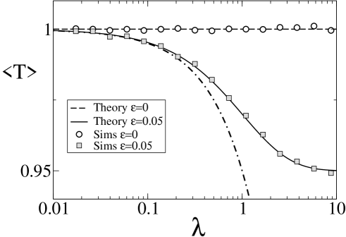
Figure 1: The mean of the first passage time vs decay rate of the exponential driving in case of a linear potential. Simulations (symbols) and theory (lines) eq. (73) with the indicated values of the driving amplitude. The dot-dashed line illustrates the slow-driving approximation eq. (75).

The variance of the FPT (Fig. 2) is always below that of the unperturbed case. It shows, remarkably, a nonmonotonous behavior as a function of the decay rate. For the parameter set used in Fig. 2, the variance attains a minimum at $\lambda\approx 1.6$. It is possible to calculate the exact location of this minimum from eq. (III.2) and express it solely by means of the mean $\langle T\rangle_{0}$ and the squared coefficient of variation (denoted for brevity by $R=CV_{0}^{2}$) of the unperturbed system

$$\lambda_{min}=\frac{\sqrt{1+4R-2R^{2}}-3R^{2}/2+4R-1}{\langle T\rangle_{0}R(2-R)^{2}}$$ (92)

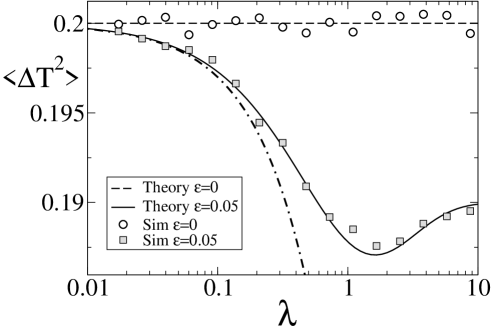
Figure 2: The variance of the first passage time vs decay rate of the exponential driving in case of a linear potential. Simulations (symbols) and theory eq. (III.2) (lines) with the indicated values of the driving amplitude. The dot-dashed line illustrates the slow-driving approximation eq. (76).

A minimum in the variance does not occur for an arbitrary parameter set but if and only if

$$R<2\;\;\Rightarrow\;\;CV_{0}=\sqrt{2D/(ax_{E})}<\sqrt{2},$$ (93)

i.e. for sufficiently weak noise intensity or large bias $a$. If the condition eq. (93) is met, the value at which the minimum is attained is an increasing function of $R$ diverging at $R=2$ and saturating for small values of the CV (i.e. $D\to 0$ or $a\to\infty$) at

$$\lambda_{min}\to\frac{3}{2}\frac{1}{\langle T\rangle_{0}}\;\;\;\mbox{as}\;\;CV_{0}\to 0.$$ (94)

The occurrence of the minimum seems to be related to the fact that a time-dependent bias reduces the variability more strongly than a shift in the initial point (corresponding to the limit $\lambda\to\infty$) does. This gives raise to the drop of the variance as $\lambda$ is decreased starting in the large-$\lambda$ limit. The amplitude of the time-dependent driving, however, depends on $\lambda$, too, so its effect on the dynamics gets weaker by further decreasing $\lambda$ and the variance starts to increase again. Accordingly, using the exponential driving without the prefactor $\lambda$ (i.e., without normalizing the driving’s intensity) yields a variance that grows monotonously with $\lambda$ (not shown). Therefore, the minimum of the variance is merely based on two competing effects, namely, the greater impact of a slow driving (compared to a fast one) on the reduction of the variance and the dependence of the variance on the driving’s amplitude (i.e. $\varepsilon\lambda$).

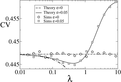
Figure 3: The coefficient of variation of the first passage time vs decay rate of the exponential driving in case of a linear potential. Simulations (symbols) and theory using eq. (13), eq. (73), and eq. (III.2) (lines) with the indicated values of the driving amplitude. The dot-dashed line illustrates the slow-driving approximation using eq. (13), eq. (75), and eq. (76).

The minimum in the variance vs $\lambda$ could be interpreted as an “optimal” decrease in variability due to an exponential driving. Things look different, though, from the view point of relative variability as it is quantified by the CV (cf. Fig. 3). First of all, depending on the value of $\lambda$, the CV can be both larger or smaller than in the unperturbed case. For the value of $\lambda$ at which the variance attains a minimum the CV is larger than in the unperturbed case and is thus far from being “optimal”. The fact that the effect of the exponential driving on the CV can be both positive or negative can be understood by looking at the CV in the limit cases of small and large decay rate where it corresponds to the CV of the unperturbed system with rescaled parameters. The latter depends on the inverse of the product $ax_{E}$. A static increase of the bias (replacing $a$ by $a+\varepsilon\lambda$ which is the effect of a slow driving) will thus lead to a decrease in CV compared to the unperturbed case (cf. the static approximation in Fig. 3). In contrast, diminishing the difference between initial point and absorbing boundary (replacing $x_{E}$ by $x_{E}-\varepsilon$ which is the effect of the forcing for $\lambda\to\infty$) leads to a higher CV than in the unperturbed case. Interpolating between the two limit cases will inevitably lead to at least one minimum of the CV vs $\lambda$. For the parameter set used in Fig. 3, this minimum is attained at a decay rate that is smaller than the inverse mean FPT of the unperturbed system.
In conclusion, already in the simple linear potential case, the effect of an exponential driving can be fairly involved. For the behavior of mean, variance, and CV as functions of the decay rate, it was essential that I have used a constant-intensity scaling of the driving function.

IV.2 Escape out of a parabolic potential with exponential forcing

With $b>0$ there is a true state dependence on the right hand side of the dynamics eq. (1). The state variable is attracted toward the potential minimum at $x=a/b$. If this rest state is far beyond the absorbing boundary $x_{E}$ (i.e. $x_{E}\ll a/b$), the FPT statistics will be similar to that of the biased random walk. In the following I choose, however, $b=1$, $a=0.8$, and $x_{E}=1$ such that $a/b<x_{E}$. With this choice the FPT problem is significantly different from the linear potential previously discussed, since in order to reach the absorbing boundary at $x_{E}=1$ the state variable $x(t)$ has to be driven by a sufficient noise to accomplish the escape out of the potential minimum.

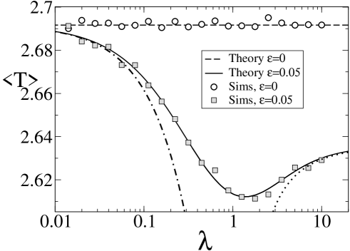
Figure 4: The mean of the first passage time vs decay rate of the exponential driving in case of a parabolic potential. Simulations (symbols) and theory eq. (86) (lines) with the indicated values of the driving amplitude. The dot-dashed line illustrates the slow-driving approximation eq. (LABEL:mean_lif_small_lam); the dotted line is the extended large-$\lambda$ approximation eq. (98).

In case of a parabolic potential, already the mean FPT depends nonmonotonously on the driving’s decay rate $\lambda$ (Fig. 4); it attains a minimum for $\lambda\approx 1.5$ which stands in marked contrast to the linear case. The reason for the occurrence of this minimum is the state dependence of the dynamics eq. (1) as I will show now. First of all, starting at $\lambda=0$, the mean FPT decreases linearly with $\lambda$ in accord with the static approximation shown by the dot-dashed line in Fig. 4. This is completely equivalent to the linear potential case. Second, the mean FPT also drops if the decay rate is decreased starting from the large-$\lambda$ limit. In other words, the limiting value is approached from below. The behavior of the mean in these two limits implies the occurrence of at least one minimum.
In order to understand why the large-$\lambda$ limit is approached from below, I consider a large but finite value of $\lambda$ and a time $t$ for which

$$\frac{1}{\lambda}\ll t\ll\langle T\rangle_{0}.$$ (95)

For such times it can be taken for granted that the driving has practically decayed to zero but on the other hand it is highly unlikely that a realization has already reached $x_{E}$. In this case the effect of the driving can be inferred from the free solution of eq. (1) for a parabolic potential with initial value $x(t=0)=0$ which can be written as follows

$$x(t)=\varepsilon\left(1+\frac{b}{\lambda-b}\right)e^{-bt}-\varepsilon\frac{\lambda}{\lambda-b}e^{-\lambda t}+\int\limits_{0}^{t}d\tilde{t}e^{b(\tilde{t}-t)}[a+\sqrt{2D}\xi(\tilde{t})]$$ (96)

If the condition eq. (95) is met, the second term can be neglected and the solution reads

$$x(t)=\varepsilon\left(1+\frac{b}{\lambda-b}\right)e^{-bt}+\int\limits_{0}^{t}d\tilde{t}e^{b(\tilde{t}-t)}[a+\sqrt{2D}\xi(t)]$$ (97)

This approximate solution is, however, equivalent to the unperturbed dynamics with an initial point at $x(t=0)=\varepsilon[1+b/(\lambda-b)]$. The equivalence holds true for a time $t$ obeying eq. (95) and any time larger than this time. In other words, for $t\gg 1/\lambda$ the realization of the original process and that of the unperturbed process with the modified initial condition differ only by a small exponential contribution. Consequently, also the FPT statistics of both processes will be the same provided that a successful escape toward $x_{E}$ is highly unlikely for short times at which eq. (97) does not hold true.
For $\lambda\to\infty$, the initial condition approaches the value $x(t=0)\to\varepsilon$ (see the discussion around eq. (90)). For a large but finite value of $\lambda$, the shift in the initial point will be larger than in the latter limit and thus the mean will be more strongly decreased than in the strict limit $\lambda\to\infty$. To obtain an explicit formula showing this drop, the mean of the unperturbed system with modified initial point is linearized with respect to $\varepsilon$ (this is not strictly necessary but consistent with the linear approach used throughout this paper) yielding

$$\langle T\rangle\approx\langle T\rangle_{0}-\varepsilon\left(1+\frac{b}{\lambda-b}\right)\sqrt{\frac{\pi}{2bD}}e^{x_{+}^{2}}\mbox{erfc}\!\left(x_{+}\right),\;\;\;\;\;\lambda\gg 1/\langle T\rangle_{0}$$ (98)

Of course, this is also obtained by replacing the amplitude $\varepsilon$ in eq. (90) by the modified amplitude $\varepsilon[1+b/(\lambda-b)]$. The approximation is shown in Fig. 4 by a dotted line; it displays the drop of the mean with decreasing $\lambda$ at large decay rate and agrees well with the full solution in this range.
I note that a nonmonotonous behavior of the mean was also found for a system with parabolic potential and a periodic forcing in ref. BulEls96 . If the system is driven by $s(t)=\varepsilon\cos(\omega t)$ the mean passes through maxima and - less pronounced - minima when plotted as a function of the driving frequency (cf. in particular Figs. 11,12, and 13 in BulEls96 ). There are two important differences between the exponential and periodic driving functions: (1) the periodic driving attains both positive and negative values; (2) the amplitude of the periodic forcing as considered in Ref. BulEls96 is fixed and does not depend on the time scale of the driving. The maxima and minima found for periodic driving are true resonance phenomena. In contrast, the minimum in the mean FPT for exponential driving appears as a compromise between the dependence of the driving’s amplitude on the decay rate (drop of the mean with increasing $\lambda$ at small $\lambda$) and the stronger effect of a truly time dependent driving on the state-dependent dynamics (drop of the mean with decreasing $\lambda$ for $\lambda\gg 1/\langle T\rangle_{0}$). I would like to point out that the latter argument does not apply in case of a linear potential (i.e., a state-independent force) because for $b=0$ the $\lambda$ dependent modification of the initial point in eq. (97) vanishes. Hence, in this case we cannot infer the existence of a minimum of $\langle T\rangle$ vs $\lambda$ and, in fact, it also does not occur as was seen in the previous subsection.

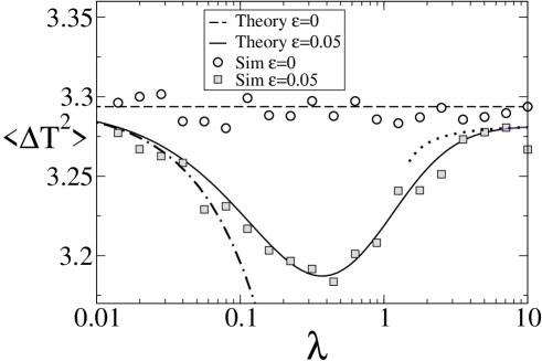
Figure 5: The variance of the first passage time vs decay rate of the exponential driving in case of a parabolic potential. Simulations (symbols) and theory eq. (87) (lines) with the indicated values of the driving amplitude. The dot-dashed line illustrates the slow-driving approximation eq. (LABEL:var_lif_small_lam); the dotted line is the extended large-$\lambda$ approximation eq. (99).

Turning to the variance depicted in Fig. 5, I note that this function also passes through a minimum vs $\lambda$ like in the linear case. This minimum occurs at a smaller decay rate ($\lambda\approx 0.38$) than that of the mean FPT and remarkably close to the inverse mean first passage time of the unperturbed system ($1/\langle T\rangle_{0}\approx 0.37$). Plotting the analytical solution eq. (87) for different parameters revealed that this time-scale matching condition holds true as long as the system is in the “subthreshold” regime, i.e. for $a/b<x_{E}$ and weak up to moderate noise intensity. For larger noise intensity and/or “suprathreshold” system parameters ($a/b>x_{E}$) the minimum is attained at values larger than $1/\langle T\rangle_{0}$. For the specific limit of weak noise and $a\to\infty$, one can expect the location at the value found for the linear potential, namely $\lambda_{min}\to 3/(2\langle T\rangle_{0})$ which is indeed larger than the inverse of the mean FPT in the unperturbed case.
The minimum of the variance can be understood by the same line of reasoning as in case of the mean, i.e. by considering the behavior at small and large-$\lambda$ which are determined by the static approximation and by the effective solution eq. (97), respectively. the latter leads - in complete analogy to the derivation of eq. (98) - to the extended large-$\lambda$ approximation of the variance

$$\langle\Delta T^{2}\rangle\!\approx\!\langle\Delta T^{2}\rangle_{0}-\varepsilon\left(1+\frac{b}{\lambda-b}\right)\sqrt{\frac{2}{Db^{3}}}\pi\!e^{x_{+}^{2}}\!\int\limits_{x_{+}}^{\infty}dx\;e^{x^{2}}\mbox{erfc}^{2}(x),\;\;\;\lambda\gg\frac{1}{\langle T\rangle_{0}}.$$ (99)

This is shown in Fig. 87 by the dotted line. I note, however, that the actual drop in variance at large $\lambda$ extends over a much larger range where eq. (99) does not hold true anymore; the decrease of the variance in this range is also much stronger than expected from eq. (99). The effect of a temporally extended driving is thus much stronger than a change of the initial point similarly to the case of a linear potential. Furthermore, because the amplitude of the driving depends on $\lambda$, the variance will drop for $\lambda\to 0$ to the value of the unperturbed system. The occurrence of the minimum is therefore mainly based on the different sensitivity of the FPT statistics with respect to changes in the bias term $a$ and the initial point of the passage and the $\lambda$ dependence of the driving amplitude due to the constant-intensity scaling of the forcing.

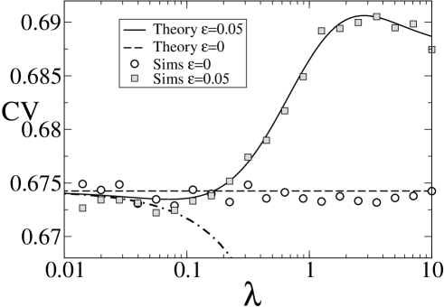
Figure 6: The coefficient of variation of the first passage time vs decay rate of the exponential driving in case of a parabolic potential. Simulations (symbols) and theory using eq. (13), eq. (86), and eq. (87) (lines) with the indicated values of the driving amplitude. The dot-dashed line illustrates the slow-driving approximation using eq. (13), eq. (LABEL:mean_lif_small_lam), and eq. (LABEL:var_lif_small_lam).

Since the minima in mean and variance vs $\lambda$ are attained at distinct values of the decay rate, I can expect a complicated behavior for the relative variability of the FPT. Indeed, the CV as a function of decay rate shown in Fig. 6 first goes through a minimum ($\lambda_{min}\approx 0.66$), reaches a maximum at a finite decay rate ($\lambda_{max}\approx 2.8$), and saturates at a CV that is higher than in the unperturbed case. Compared to the CV of the linear potential system (cf. Fig. 3), the decrease at small $\lambda$ is weaker; furthermore, there is no maximum for the linear system but only a saturation at large decay rate.
For the chosen parameters the FPT from $x=0$ to $x=x_{E}$ can be split into two independent FPTs as $T=T_{1}+T_{2}$ with $T_{1}$ being the FPT from $x=0$ into the minimum $x=a/b$ and $T_{2}$ being the time for the passage from the minimum to the absorbing boundary (see, for instance, ref. PakTan01 ). It is straightforward to show that

$$CV^{2}=CV_{1}\frac{\langle T_{1}\rangle^{2}}{\langle T\rangle^{2}}+CV_{2}\frac{\langle T_{2}\rangle^{2}}{\langle T\rangle^{2}}$$ (100)

where $CV_{1}$ and $CV_{2}$ are the CV of the respective passage processes. Now the relaxation into the minimum is evidently more regular than the noise-assisted escape out of the potential minimum, i.e. $CV_{2}>CV_{1}$. The behavior of the CV can be understood by considering how in the limits of small and large decay rate the relative contributions of $T_{1}$ and $T_{2}$ are changed.
At low decay rate, the driving is effectively static, hence the system is equivalent to the unperturbed dynamics with enlarged bias $a+\varepsilon\lambda$. This system in turn is equivalent to the unperturbed dynamics with the original bias $a$ but initial point at $x=-\varepsilon\lambda$ and absorbing boundary at $x=x_{E}-\varepsilon\lambda$. With these parameters, the FPT $T_{1}$ from initial point to potential minimum increases and the FPT $T_{2}$ from minimum to absorbing boundary drops compared to the unperturbed case. It is reasonable that the CV of the single passage processes change only little; what mainly changes is their relative contribution to the total CV by means of the squared ratios $T_{1}/T$ and $T_{2}/T$. Hence, according to eq. (100) the CV will drop since the lower CV of $T_{1}$ makes a larger relative contribution. From this line of argument, it is also reasonable that the CV drops with increasing $\lambda$ as long as the static approximation holds true.
In the limit of $\lambda\gg\langle T\rangle$, one obtains also the unperturbed dynamics (as explained above by means of eq. (97)) but for a passage process from $x=\varepsilon[1+b/(\lambda-b)]$ to $x=x_{E}$. Obviously, here the escape time $T_{2}$ is the same as in the unperturbed case; the first FPT $T_{1}$, however, has been shortened. According to eq. (100), one can thus expect a higher CV than in the unperturbed case since $CV_{2}$ makes a larger relative contribution to the CV of the total FPT. Moreover, the $\lambda\to\infty$ limit of the CV is approached from above because the shift in initial point drops with increasing $\lambda$. Interpolating in the simplest way between the behavior at small and large $\lambda$ predicts a minimum at moderately low decay rate and a maximum at larger rate as has been found in Fig. 6. I note that for the decay rate at which the variance attains a minimum, the CV is higher than in the unperturbed case, similarly to the linear potential case ($b=0$) discussed in the previous subsection.
Like in case of the biased random walk, the behavior of mean and variance as functions of the decay rate depends crucially on the constant-intensity scaling of the driving I have used. Additionally, the state-dependence of the force leads to a nonmonotonous behavior of the mean as a function of the decay rate. The minima in mean and variance are not true resonances as in case of a periodic driving but are mainly related to the distinct sensitivity of the FPT statistics with respect to changes in the initial point or in the bias parameter, respectively. Nevertheless, in physical situations where a constant-intensity scaling of the driving is appropriate, the nonmonotonous behavior of the first two cumulants and of the CV may be of some importance.

V Summary and outlook

In this paper I have studied the moments of the first passage time in presence of a weak time-dependent driving. A formula for the corrections to the moments for arbitrary driving and potential shape were derived that contains, however, the time-dependent probability density of the unperturbed system or its Laplace transform. The latter functions are known only in a few rare cases. Explicite correction formulas for mean and variance of the first passage time could be achieved for the case of an exponentially decaying driving function and an either linear or parabolic potential. These analytical results were found to be in excellent agreement with results from computer simulations of the passage processes. I demonstrated furthermore, that for the chosen exponential driving, the variance of the passage time in the linear case as well as both the mean and the passage time in case of a parabolic potential pass through minima as functions of the decay rate of the driving. The behavior of the relative standard deviation (i.e. the CV) proved to be even more complicated. All of these findings resemble the effects of coherent stochastic resonance and resonant activation, however, they rely on a different mechanism involving the constant-intensity scaling of the driving.
The explicit results for the case of a linear or a parabolic potential derived in this paper will be applied in the near future to the neurobiological problems mentioned in the introduction. Furthermore, the results can be useful for other problems, too. The application of the formulas to the case of a periodic driving with a cosine function studied in Refs. BulLow94 ; GitWei95 ; BulEls96 is straightforward. Likewise, the case of an exponentially damped cosine function involving two time scales (driving period and decay rate) can be readily derived from my formulas and might be worth to look at.
The general approach presented in this paper may be easily extended to the cases of two absorbing boundaries or one absorbing and one reflecting boundary. I am also convinced that the problem of a state-dependent driving (i.e. dealing with a force $s(x,t)$ instead of $s(t)$) can be successfully treated with the approach. Finally, the case of a stochastic driving function might be tackled by a proper average of the correction formulas over the driving process and its initial condition. This last problem, though, seems to be much more challenging than the other extensions of the theory.

VI Acknowledgment

I am indebted to André Longtin for inspiring discussions that brought the subject of this paper to my attention; I furthermore wish him to thank for his generous support during the last years. This work has been supported by NSERC Canada.

Appendix A Equivalence of the different quadratures expressions

Here I show that eq. (27) together with eq. (24) and eq. (16) yields the same FPT moments as the standard formula eq. (9). The two differing expressions for the $n$-th moment can be written as follows (indices “S” and “A” stand for “standard” and “alternative”)

$$\langle T^{n}\rangle_{S} = \frac{n}{D^{n}}\!\!\!\int\limits_{a}^{b}\!\!dy_{1}e^{\frac{U(y_{1})}{D}}\!\!\!\int\limits_{-\infty}^{y_{1}}\!\!dx_{1}e^{-\frac{U(x_{1})}{D}}\!\!\!\int\limits_{x_{1}}^{b}\!\!dy_{2}e^{\frac{U(y_{2})}{D}}\!\!\!\int\limits_{-\infty}^{y_{2}}\!\!dx_{2}e^{-\frac{U(x_{2})}{D}}\cdots$$ (101)

$$\hskip 30.00005pt\cdots\int\limits_{x_{n-1}}^{b}\!\!dy_{n}e^{\frac{U(y_{n})}{D}}\!\!\!\int\limits_{-\infty}^{y_{n}}\!\!dx_{n}e^{-\frac{U(x_{n})}{D}}$$

$$\langle T^{n}\rangle_{A} = \frac{n}{D^{n}}\!\!\!\int\limits_{-\infty}^{b}\!\!dy_{1}e^{-\frac{U(y_{1})}{D}}\!\!\!\int\limits_{y_{1}}^{b}\!\!dx_{1}e^{\frac{U(x_{1})}{D}}\!\!\!\int\limits_{-\infty}^{x_{1}}\!\!dy_{2}e^{-\frac{U(y_{2})}{D}}\!\!\!\int\limits_{y_{2}}^{b}\!\!dx_{2}e^{\frac{U(x_{2})}{D}}\cdots$$ (102)

$$\hskip 30.00005pt\cdots\int\limits_{-\infty}^{x_{n-1}}\!\!dy_{n}e^{-\frac{U(y_{n})}{D}}\!\!\!\int\limits_{y_{n}}^{b}\!\!dx_{n}e^{\frac{U(x_{n})}{D}}\Theta(x_{n}-a)$$

Note that for the second formula, I have used an arbitrary initial point $x(t=0)=a$ which only changes the argument of the Heaviside function in eq. (24).
Now I introduce the operators

$${\hat{\cal K}}_{x_{j}}(x) = \int\limits_{x_{j}}^{b}dy\;e^{U(y)/D}\int\limits_{-\infty}^{y}dxe^{-U(x)/D}$$ (103)

$${\hat{\cal M}}_{x_{j}}(x) = \int\limits_{-\infty}^{x_{j}}dy\;e^{-U(y)/D}\int\limits_{y}^{b}dxe^{U(x)/D}$$ (104)

where the argument indicates the variable with respect to which the respective function is integrated, while the index denotes as a parameter one boundary of integration. It is not hard to show that for $u,w<b$

$${\hat{\cal M}}_{u}(v)\Theta(v-w)={\hat{\cal K}}_{w}(v)\Theta(u-v).$$ (105)

and

$${\hat{\cal M}}_{u}(v){\hat{\cal K}}_{w}(x)={\hat{\cal K}}_{w}(x){\hat{\cal M}}_{u}(v),$$ (106)

i.e., the operators commute if their arguments and indices differ.
By means of the operators, the two expressions for the $n$-th moment can be written as follows

$$\langle T^{n}\rangle_{S} = \frac{n}{D^{n}}{\hat{\cal K}}_{a}(x_{1}){\hat{\cal K}}_{x_{1}}(x_{2})\cdots{\hat{\cal K}}_{x_{n-1}}(x_{n})\Theta(b-x_{n})$$ (107)

$$\langle T^{n}\rangle_{A} = \frac{n}{D^{n}}{\hat{\cal M}}_{b}(x_{1}){\hat{\cal M}}_{x_{1}}(x_{2})\cdots{\hat{\cal M}}_{x_{n-1}}(x_{n})\Theta(x_{n}-a)$$ (108)

Note that the function $\Theta(b-x_{n})$ in eq. (107) is always one since $x_{j}<b$ for all $j=1,\dots n$. Using the relations eq. (105) and eq. (106) it follows from eq. (108) that

$$\langle T^{n}\rangle_{A} = \frac{n}{D^{n}}{\hat{\cal M}}_{b}(x_{1})\cdots{\hat{\cal M}}_{x_{n-2}}(x_{n-1}){\hat{\cal K}}_{a}(x_{n})\Theta(x_{n-1}-x_{n}),$$ (109)

$$= \frac{n}{D^{n}}{\hat{\cal M}}_{b}(x_{1})\cdots{\hat{\cal M}}_{x_{n-3}}(x_{n-2}){\hat{\cal K}}_{a}(x_{n}){\hat{\cal K}}_{x_{n}}(x_{n-1})\Theta(x_{n-2}-x_{n-1}),$$

$$\frac{}{}\vdots,$$

$$= \frac{n}{D^{n}}{\hat{\cal K}}_{a}(x_{n})\cdots{\hat{\cal K}}_{x_{2}}(x_{1})\Theta(b-x_{1})$$

$$= \langle T^{n}\rangle_{S}$$

as it should be.

References

- [1] L. Pontryagin, A. Andronov, and A. Witt. Zh. Eksp. Teor. Fiz., 3:172, 1933. Reprinted in Noise in Nonlinear Dynamical Systems, 1989, ed. by F. Moss and P. V. E. McClintock (Cambridge University Press, Cambridge), Vol. 1, p. 329.
- [2] A. J. F. Siegert. On the first passage time problem. Phys. Rev., 81:617, 1951.
- [3] M. Bier and R. D. Astumian. Matching a diffusive and a kinetic approach for escape over an fluctuating barrier. Phys. Rev. Lett., 71:1649, 1993.
- [4] C. R. Doering and J. C. Gadoua. Resonant activation over a fluctuating barrier. Phys. Rev. Lett., 16:2318, 1992.
- [5] P. Pechukas and P. Hänggi. Rates of activated processes with fluctuating barriers. Phys. Rev. Lett., 73:2772, 1994.
- [6] P. Reimann. Thermally driven escape with fluctuating potentials: A new type of resonant activation. Phys. Rev. Lett., 23:4576, 1995.
- [7] L. Gammaitoni, P. Hänggi, P. Jung, and F. Marchesoni. Stochastic resonance. Rev. Mod. Phys., 70:223, 1998.
- [8] J. E. Fletcher, S. Havlin, and G. H. Weiss. First passage time problems in time-dependent fields. J. Stat. Phys., 51:215, 1988.
- [9] M. Gitterman and G. H. Weiss. Coherent stochastic resonance in the presence of a field. Phys. Rev. E, 52:5708, 1995.
- [10] J. Masoliver, A. Robinson, and G. H. Weiss. Coherent stochastic resonance. Phys. Rev. E, 51:4021, 1995.
- [11] J. M. Porrá. When coherent stochastic resonance appears. Phys. Rev. E, 55:6533, 1997.
- [12] B. Lindner and A. Longtin. Nonrenewal spike trains generated by stochastic neuron models. In L. Schimansky-Geier, D. Abbott, A. Neiman, and Ch. Van den Broeck, editors, Noise in Complex Systems and Stochastic Dynamics, volume 5114, page 209, Bellingham, Washington, 2003. SPIE.
- [13] M. J. Chacron, A. Longtin, M. St-Hilaire, and L. Maler. Suprathreshold stochastic firing dynamics with memory in P-type electroreceptors. Phys. Rev. Lett., 85:1576, 2000.
- [14] M. J. Chacron, K. Pakdaman, and A. Longtin. Interspike interval correlations, memory, adaptation, and refractoriness in a leaky integrate-and-fire model with threshold fatigue. Neural Comp., 15:253, 2003.
- [15] A. Bulsara, T. C. Elston, Ch. R. Doering, S. B. Lowen, and K. Lindenberg. Cooperative behavior in periodically driven noisy integrate-and-fire models of neuronal dynamics. Phys. Rev. E, 53:3958, 1996.
- [16] A. Bulsara, S. B. Lowen, and C. D. Rees. Cooperative behavior in the periodically modulated Wiener process: Noise-induced complexity in a model neuron. Phys. Rev. E, 49:4989, 1994.
- [17] P. Lánský. Sources of periodical force in noisy integrate-and-fire models of neuronal dynamics. Phys. Rev. E, 55:2040, 1997.
- [18] H. E. Plesser and T. Geisel. Stochastic resonance in neuron models: Endogenous stimulation revisited. Phys. Rev. E, 63:031916, 2001.
- [19] H. E. Plesser and S. Tanaka. Stochastic resonance in a model neuron with reset. Phys. Lett. A, 225:228, 1997.
- [20] A. Longtin. Stochastic resonance in neuron models. J. Stat. Phys., 70:309, 1993.
- [21] V. Bezak. The first-passage-time problems with time-varying driving fields. Acta Phys. Slov., 39:337, 1989.
- [22] V. Balakrishnan, C. Van den Broeck, and P. Hänggi. First-passage times of non-markovian processes:The case of a reflecting boundary. Phys. Rev. A, 38:4213, 1988.
- [23] S. Redner. A Guide to First-Passage Processes. Cambridge University Press, Cambridge, UK, 2001.
- [24] M. H. Choi and R. F. Fox. Evolution of escape processes with a time-varying load. Phys. Rev. E, 66:031103, 2002.
- [25] S. V. G. Menon. First passage time distribution in an oscillating field. J. Stat. Phys., 66:1675, 1992.
- [26] I. Klik and Y. D. Yao. Resonant activation in a system with deterministic oscillations of barrier height. Phys. Rev. E, 64:012101, 2001.
- [27] R. Gutiérrez, L. M. Ricciardi, P. Román, and F. Torres. First-passage-time densities for time-non-homogeneous diffusion processes. J. Appl. Prob., 34:623, 1997.
- [28] R. Gutiérrez Jáimez, A. Juan Gonzalez, and P. Román Román. Construction of first-passage-time densities for a diffusion process which is not necessarily time-homogeneous. J. Appl. Prob., 28:903, 1991.
- [29] R. Gutiérrez Jáimez, P. Román Román, and F. Torres Ruiz. A note on the Volterra integral equation for the first-passage-time probability density. J. Appl. Prob., 32:635, 1995.
- [30] J. Lehmann, P. Reimann, and P. Hänggi. Surmounting oscillating barriers. Phys. Rev. Lett., 84:1639, 2000.
- [31] V. N. Smelyanski, M. I. Dykman, and B. Golding. Time oscillations of escape rates in periodically driven systems. Phys. Rev. Lett., 82:3193, 1999.
- [32] P. Talkner and J. Łuczka. Rate description of Fokker-Planck processes with time dependent parameters. cond-mat/0307498, 2003.
- [33] A. I. Shushin. Effect of external force on the kinetics of diffusion-controlled escaping from a one-dimensional potential well. Phys. Rev. E, 62:4688, 2000.
- [34] P. Hänggi, P. Talkner, and M. Borkovec. Reaction rate theory: Fifty years after kramers. Rev. Mod. Phys., 62:251, 1990.
- [35] H. A. Kramers. Brownian motion in a field of force and the diffusion model of chemical reactions. Physica, 7:284, 1940.
- [36] C. W. Gardiner. Handbook of Stochastic Methods. Springer-Verlag, Berlin, 1985.
- [37] A. V. Holden. Models of the Stochastic Activity of Neurones. Springer-Verlag, Berlin, 1976.
- [38] M. Abramowitz and I. A. Stegun. Handbook of Mathematical Functions. Dover, New York, 1970.
- [39] N. G. Van Kampen. Short first-passage times. J. Stat. Phys., 70:15, 1993.
- [40] B. Lindner, L. Schimansky-Geier, and A. Longtin. Maximizing spike train coherence or incoherence in the leaky integrate-and-fire model. Phys. Rev. E, 66:031916, 2002.
- [41] J. Honerkamp. Stochastic Dynamical Systems. Concepts, Numerical Methods, Data Analysis. Wiley/VCH, Weinheim, 1993.
- [42] K. Pakdaman, S. Tanabe, and T. Shimokawa. Coherence resonance and discharge reliability in neurons and neuronal models. Neural Networks, 14:895, 2001.