Surface Superconductivity of Dirty Two-Band Superconductors: Applications to ${\rm MgB}_{2}$.

Abstract

The minimal magnetic field $H_{c2}$ destroying superconductivity in the bulk of a superconductor is smaller than the magnetic field $H_{c3}$ needed to destroy surface superconductivity if the surface of the superconductor coincides with one of the crystallographic planes and is parallel to the external magnetic field. While for a dirty single-band superconductor the ratio of $H_{c3}$ to $H_{c2}$ is a universal temperature-independent constant 1.6946, for dirty two-band superconductors this is not the case. I show that in the latter case the interaction of the two bands leads to a novel scenario with the ratio $H_{c3}/H_{c2}$ varying with temperature and taking values larger and smaller than 1.6946. The results are applied to ${\rm MgB}_{2}$ and are in agreement with recent experiments [A. Rydh et al., cond-mat/0307445].

Introduction. It is well-established that strong magnetic field destroys superconductivity. If an external field $H$ applied to a type-II superconductor exceeds the second critical field $H_{c2}$, the bulk order parameter in the superconductor vanishes. However, even for $H>H_{c2}$ superconductivity might still exist in a thin layer close to the surface if $H$ is smaller than the third critical field $H_{c3}>H_{c2}$Saintjames . In this paper I investigate the onset of superconductivity via surface nucleation for the field $H$ slightly below the threshold $H_{c3}$.

In their pioneering workSaintjames Saint-James and de Gennes have shown that if the external magnetic field is applied parallel to the surface of an isotropic single-band superconductorfootnote_1 with a temperature close to the transition temperature $T_{c}$, the ratio $H_{c3}/H_{c2}$ takes the universal value $\eta=1.6946$ independently of the superconducting material. It turns outSaintjames that for $H$ slightly below $H_{c3}$ the superconducting order parameter exists within the distance $\zeta(T)$ (the coherence length of the superconductor) from the surface. For distances exceeding $\zeta(T)$ the order parameter approaches zero rapidly. The dependence of the ratio $H_{c3}/H_{c2}$ on the material propertiesSaintjames_book ; Degennes_book ; Strongin , sample geometry and topologyKogan ; Saintjames_2 ; Moshchalkov , and temperatureAbrikosov ; Kulik ; Keller has become a subject of intensive investigations.

A novel window for investigating surface superconductivity was opened after the discovery of the two-band superconductor ${\rm MgB}_{2}$Nagamatsu . Not only has it a relatively high ($\approx 40$ K) $T_{c}$ but also there exist two different superconducting gaps. As the consequence of this fact, various properties of ${\rm MgB}_{2}$ are quite different from those of single-band superconductors. For example, the anisotropy $\gamma(T)=H_{c2}^{(ab)}(T)/H_{c2}^{(c)}(T)$ (here, $H_{c2}^{(ab)}(T)$ and $H_{c2}^{(c)}(T)$ stand for the second critical fields in the $ab$ and $c$-directions respectively; note that the crystal of ${\rm MgB}_{2}$ is uniaxial) of the second critical field ${\rm H}_{c2}$ exhibits strong dependence on temperature, see e.g. Ref. Angst . For single-band superconductors this ratio is constant.

Another puzzle is that $\gamma(T)$ varies widely in different experimentsWelp . This can be attributed to the existence of surface superconductivity which might affect the observable values of $H_{c2}$ and, hence, the anisotropy. Consequently, the determination of the third critical field $H_{c3}$ is a very important problem. In a recent experimentRydh it has been shown that $H_{c3}/H_{c2}$ for ${\rm MgB}_{2}$ might be reduced.

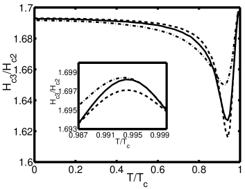
Figure 1: $H_{c3}/H_{c2}$ for the surface of the ${\rm MgB}_{2}$ crystal coinciding with the $ab$-plane and the external magnetic field lying in the $ab$-plane for different ratios of the diffusivities $D_{2,c}/D_{1,c}=100,300,600$ in the two bands (dash-dot, solid, and dashed respectively) as a function of $T/T_{c}$. Inset: $H_{c3}/H_{c2}$ close to $T/T_{c}=1$. For $T=T_{c}$, $H_{c3}/H_{c2}=1.6946$.

In the present paper I investigate the ratio $H_{c3}/H_{c2}$ for a dirty ${\rm MgB}_{2}$ crystal. The existence of two different gaps manifests itself through the remarkable dependence of $H_{c3}/H_{c2}$ on temperature. This is in sharp contrast with the case of a dirty single-gap superconductor where $H_{c3}/H_{c2}=\eta$ in the whole temperature range. For a magnetic field lying in the $ab$-plane of the ${\rm MgB}_{2}$ crystal I find that if one starts decreasing temperature, $H_{c3}/H_{c2}$ first exhibits a maximum at $T\approx 0.99T_{c}$ and then a minimum at $T\approx 0.9T_{c}$. As temperature decreases further, $H_{c3}/H_{c2}$ increases and tends to a value slightly below $\eta$, see Fig. 1. Naively, one could try to use the Ginzburg-Landau theory (GLT) in order to find $H_{c3}/H_{c2}$. However, as it will be explained below, this would lead to the ratio $H_{c3}/H_{c2}=\eta$ in the whole temperature range, i.e. one needs a more rigorous approach in order to explain the deviation of $H_{c3}/H_{c2}$ from $\eta$.

General formalism. An appropriate tool to investigate magnetic properties of dirty superconductors is the Usadel equationsUsadel . For two-band superconductors they have been derived by Koshelev and GolubovKoshelev and by GurevichGurevich . Since I investigate the onset of superconductivity near $H_{c2}$ or $H_{c3}$, it is possible to write the Usadel equations in the linearized form

$$\omega f_{\alpha}+\left(-\sum\limits_{j}\frac{D_{\alpha,j}}{2}{\left(\nabla_{j}-\frac{2\pi i}{\Phi_{0}}A_{j}\right)}^{2}\right)f_{\alpha}=\Delta_{\alpha}$$ (1)

$$\Delta_{\alpha}=2\pi T\sum\limits_{\omega>0}^{\omega_{D}}\Lambda_{\alpha\beta}f_{\beta}$$ (2)

Here, $\omega=2\pi T(n+1/2),n=0,1,\dots$ and $\omega_{D}$ are the Matsubara and cutoff phonon frequencies. $D_{\alpha,j}$ is the diffusion coefficient of the band $\alpha=1,2$ along the direction $j=x,y,z$. The indices 1 and 2 correspond to the $\sigma$- and $\pi$-bands respectively. ${\bf A}$ is the vector potential. $\Delta_{\alpha}$ and $f_{\alpha}$ are the superconducting gap and anomalous green function for the band $\alpha$. The matrix ${\hat{\Lambda}}$ represents the strength of the coupling parameters and has the values $\lambda_{11}\approx 0.81$, $\lambda_{22}=0.285$, $\lambda_{12}\approx 0.119$, and $\lambda_{21}\approx 0.09$, see Ref. Mazin . In the present paper I will concentrate on two geometries: i) the magnetic field is parallel to the $c$-axis and the surface of the crystal; ii) the surface of the superconductor coincides with the $ab$-plane and the field H lies in the $ab$-plane. As I will show, in case i $H_{c3}/H_{c2}=\eta$ at any temperature. In case ii, $H_{c3}/H_{c2}$ is shown in Fig. 1. I assume that ${\bf H}$ is parallel to the $z$-axis.

Choosing the gauge as $A_{y}=Hx$ I look for the solution of the form $f_{\alpha}\equiv f_{\alpha}(\omega,x)\exp\left(ik_{y}y+ik_{z}z\right)$ and $\Delta_{\alpha}\equiv\Delta_{\alpha}(x)\exp\left(ik_{y}y+ik_{z}z\right)$. In general, Eqs. (1) and (2) define a sequence of solutions corresponding to different eigenvalues $H=H_{c2}$ or $H=H_{c3}$. One should look for the maximal possible values of $H_{c2}$ or $H_{c3}$. This corresponds to the case $k_{z}=0$. Substituting the Ansatz for $f_{\alpha}$ and $\Delta_{\alpha}$ into (1) and (2) I obtain the system of equations

$${\hat{\Lambda}}^{-1}\left(\begin{array}[]{c}\Delta_{1}(x)\\ \Delta_{2}(x)\end{array}\right)=\left(\begin{array}[]{cc}2\pi T\sum\limits_{\omega>0}^{\omega_{D}}\frac{1}{\omega+{\hat{H}}_{1}(x_{0})}&0\\ 0&2\pi T\sum\limits_{\omega>0}^{\omega_{D}}\frac{1}{\omega+{\hat{H}}_{2}(x_{0})}\end{array}\right)\left(\begin{array}[]{c}\Delta_{1}(x)\\ \Delta_{2}(x)\end{array}\right),$$ (3)

where

$${\hat{H}}_{\alpha}(x_{0})=-\frac{{\tilde{D}}_{\alpha,x}}{2}\frac{\partial^{2}}{\partial x^{2}}+\frac{{\tilde{D}}_{\alpha,z}}{2}{\left(\frac{2\pi H}{\Phi_{0}}\right)}^{2}{\left(x-x_{0}\right)}^{2},$$ (4)

with ${\tilde{D}}_{\alpha,x}={\tilde{D}}_{\alpha,z}={D}_{\alpha,a}$ for case i and ${\tilde{D}}_{\alpha,x}=D_{\alpha,a}$ and ${\tilde{D}}_{\alpha,z}=D_{\alpha,c}$ for case ii ($D_{\alpha,a}=D_{\alpha,b}\neq D_{\alpha,c}$ are the diffusion coefficients along the crystallographic axes). $x_{0}=k_{y}\Phi_{0}/2\pi H$ is the parameter characterizing how far away the superconducting nucleus is situated from the surface. Note that $x_{0}$ is the same for the both bands. The operator (4) can be rewritten in the form $\left(\pi H/\Phi_{0}\right)\sqrt{{\tilde{D}}_{\alpha,x}{\tilde{D}}_{\alpha,z}}{\hat{h}}_{\alpha}(x_{0}^{\prime})$, with

$${\hat{h}}_{\alpha}(x_{\alpha,0}^{\prime})=-\frac{\partial^{2}}{\partial{x_{\alpha}^{\prime}}^{2}}+{\left(x_{\alpha}^{\prime}-x_{\alpha,0}^{\prime}\right)}^{2},$$ (5)

where I have made the variable substitution $x=\beta_{\alpha}x_{\alpha}^{\prime}$ and $x_{0}=\beta_{\alpha}x_{\alpha,0}^{\prime}$, with $\beta_{\alpha}={\left({\tilde{D}}_{\alpha,x}/{\tilde{D}}_{\alpha,z}\right)}^{1/4}{\left(\Phi_{0}/2\pi H\right)}^{1/2}$.

The system (3) should be solved with the boundary conditions (BC) $\partial\Delta_{\alpha}/\partial x|_{x=0}=0$, and $\Delta_{\alpha}(x\rightarrow+\infty)\rightarrow 0$, $\alpha=1,2$ valid for geometries i and ii, see above. For $H_{c3}$ the BC are well-established for dirty superconductorsDegennes_book . For $H_{c2}$ the application of these BC gives the same result as the BC requiring the appearance of a superconducting nucleus in the bulk. The procedure of finding $H_{c3}/H_{c2}$ is following: first, set $x_{0}=0$ in (3) and find the maximal possible field $H$ for which the solution satisfying the BC exists. This gives $H_{c2}$. Next, for $x_{0}\neq 0$ find the maximal field $H=H(x_{0})$ for which the solution of (3) exists. Then, $H_{c3}={\rm max}_{x_{0}}\left\{H(x_{0})\right\}$. I would like to mention that there are complementary approaches for calculating $H_{c2}$ based on macroscopic theoryMiranovic ; Dahm and GLTAskerzade ; Zhitomirsky .

Here, it is instructive to study briefly the case of a single-gap superconductor. This corresponds to $\lambda_{12}=\lambda_{21}=0$. $H_{c2}$ and $H_{c3}$ are then determined by those for band 1 (as $\lambda_{11}>\lambda_{22}$). The solution for $\Delta_{1}(x)$ is proportional to the ground state wave function of the operator ${\hat{H}}_{1}(x_{0})$ and $\Delta_{2}(x)=0$. Substituting this Ansatz into (3) I obtain the transcendental equation of the form

$$1-\lambda_{11}\sum_{\omega>0}^{\omega_{D}}\frac{1}{\omega+\left(\pi H/\Phi_{0}\right)\sqrt{{\tilde{D}}_{1,x}{\tilde{D}}_{1,z}}\epsilon_{0}(x_{1,0}^{\prime})}=0,$$ (6)

with $\epsilon_{0}(x_{\alpha,0}^{\prime})$ the lowest eigenvalue of the operator ${\hat{h}}_{\alpha}(x_{\alpha,0}^{\prime})$. The field $H_{c2}$ can be found as the solution of the above equation for $x_{1,0}^{\prime}=0$; note that $\epsilon_{0}(0)=1$. Assume, a certain value of the magnetic field $H_{c2}$ is found; let us change the parameter $x_{1,0}^{\prime}$. This leads to the decrease of the eigenvalue $\epsilon_{0}(x_{1,0}^{\prime})$Saintjames . In order to satisfy Eq. (6) one has to increase the field $H$; that is why $H_{c3}>H_{c2}$. The minimal $\epsilon_{0}(x_{1,0}^{\prime})$ can be realized for $x_{1,0}^{\prime}=0.7618$Saintjames and is equal to $0.5901$Saintjames . This means that $H_{c3}/H_{c2}=1/0.5901=\eta$ for any temperature $T$. Remarkably, it is not necessary to solve Eq. (6) in order to find the ratio $H_{c3}/H_{c2}$, although the determination of $H_{c2}$ or $H_{c3}$ alone would require the complete analysis.

Case i. In this case, the ratio $H_{c3}/H_{c2}=\eta$ at all temperatures. This is a consequence of the fact that the operators ${\hat{H}}_{1}(x_{0})$ and ${\hat{H}}_{2}(x_{0})$ have identical eigenfunctions (since ${\tilde{D}}_{1,x}/{\tilde{D}}_{1,z}={\tilde{D}}_{2,x}/{\tilde{D}}_{2,z}=1$). The functions $\Delta_{1}(x)$ and $\Delta_{2}(x)$ are proportional to the ground state wave function of the operator ${\hat{H}}_{1}(x_{0})$ (or ${\hat{H}}_{2}(x_{0})$). The equation determining the critical fields $H_{c2}$ and $H_{c3}$ has the form $F\left(\pi D_{1,a}H\epsilon_{0}(x_{1,0}^{\prime})/\Phi_{0},\thinspace\pi D_{2,a}H\epsilon_{0}(x_{2,0}^{\prime})/\Phi_{0}\right)=0$, with $F(y_{1},y_{2})$ a certain function of two arguments. Note that in the present case $\beta_{1}=\beta_{2}$ and, consequently, $x_{1,0}^{\prime}=x_{2,0}^{\prime}$ and $\epsilon_{0}(x_{1,0}^{\prime})=\epsilon_{0}(x_{2,0}^{\prime})$. The maximal value of $H_{c3}$ can be realized for $x_{1,0}^{\prime}=0.7618$ and is equal to $\eta H_{c2}$ for all temperatures.

Case ii. If the magnetic field lies in the $ab$-plane, the operators ${\hat{H}}_{1}(x_{0})$ and ${\hat{H}}_{2}(x_{0})$ have different eigenfunctions. This leads to a complicated transcendental equation depending on all eigenvalues of the operators ${\hat{H}}_{1}(x_{0})$ and ${\hat{H}}_{2}(x_{0})$ and not only on the ground state ones. Eqs. (3) can be solved via expanding functions $\Delta_{1}(x)$ and $\Delta_{2}(x)$ over the eigenfunctions of the operators ${\hat{H}}_{1}(x_{0})$ and ${\hat{H}}_{2}(x_{0})$. I have truncated the basis of the operators ${\hat{H}}_{1}(x_{0})$ and ${\hat{H}}_{2}(x_{0})$ to subspaces consisting of 70 eigenfunctions and solved the system (3) numerically. In Fig. 1 I show the results of the numerics. Here, I take $D_{1,a}/D_{1,c}=40.0$, $D_{2,a}/D_{2,c}=0.665$. These ratios can be obtained using the results for the average velocity on the ${\rm MgB}_{2}$ Fermi surfaces and assuming isotropic scattering, see Refs. Golubov ; Brinkman . The ratio $D_{2,c}/D_{1,c}$ takes three values: 100, 300, and 600. This choice is motivated by the facts that the ratio $D_{2,c}/D_{1,c}\approx 100$ can be obtained assuming that the scattering rate of electrons is the same in both bands. On the other hand $R=D_{2,c}/D_{1,c}=600$ gives a better fit with experiments on the anisotropy measurementsGolubov .

The results are shown in Fig. 1. For temperatures $T\lesssim 0.6T_{c}$ I have found that the ratio $H_{c3}/H_{c2}$ is nearly constant and has a value slightly below $\eta$. This can be explained by the fact that at low temperatures the fields $H_{c2}$ and $H_{c3}$ are determined mostly by the $\sigma$-band whose coherence length is much smaller than that of the $\pi$-band. At low $T$ the magnetic field $H_{c2}$ depends on the ground state eigenvalues of the operators ${\hat{H}}_{1}(x_{0})$ and ${\hat{H}}_{2}(x_{0})$ and the contribution of excited states is negligibleGurevich ; Koshelev . The ratios ${\left({\tilde{D}}_{1,x}/{\tilde{D}}_{1,z}\right)}^{1/4}$ and ${\left({\tilde{D}}_{2,x}/{\tilde{D}}_{2,z}\right)}^{1/4}$ determining the length $x_{0}$ are equal to $\approx 2.5$ and $0.9$ respectively. This means that one can maximize the field $H_{c3}$ by choosing $x_{1,0}^{\prime}=0.7618$. The length $x_{2,0}^{\prime}$ then is large and the ground-state eigenvalue of the operator ${\hat{h}}_{2}(x_{2,0}^{\prime})$ is close to $1$. The ratio $H_{c3}/H_{c2}$ then can be calculated as follows: take the zero temperature expression for $H_{c2}$Gurevich ; Golubov and make there a substitution $D_{1,j}\rightarrow D_{1,j}/\eta$. At low temperaturesGurevich ; Golubov , $H_{c2}={\Phi_{0}T_{c}\exp\left(g/2\right)}/{2\gamma{\left(D_{1,a}D_{1,c}D_{2,a}D_{2,c}\right)}^{1/4}},$ with $g={\left({\lambda_{0}^{2}}/{w^{2}}+{\ln^{2}\kappa}/{4}+{{2\lambda_{-}}\ln\kappa}/{w}\right)}^{1/2}-{\lambda_{0}}/{w},$ $\kappa={D_{2,a}D_{2,c}}/{D_{1,a}D_{1,c}}$, $\lambda_{-}=\lambda_{11}-\lambda_{22}$, $\lambda_{0}={\left(\lambda_{-}^{2}+4\lambda_{12}\lambda_{21}\right)}^{1/2}$, $w=\lambda_{11}\lambda_{22}-\lambda_{12}\lambda_{21}$, and $\ln\gamma=0.5772$. This procedure yields $H_{c3}/H_{c2}=1.688,1.690,$ and $1.691$ for $D_{2,c}/D_{1,c}=100,300,$ and $600$ respectively. The values obtained in the numerics are slightly larger (but still smaller than $\eta$) due to a small contribution to the adjustment of $x_{0}$ from the $\pi$-band.

If one increases temperature, the ratio $H_{c3}/H_{c2}$ decreases and exhibits a minimum at $T\simeq 0.9T_{c}$. Then, the value of $H_{c3}/H_{c2}$ goes up and takes a maximum at $T\simeq 0.99T_{c}$. At $T=T_{c}$, $H_{c3}/H_{c2}=\eta$. The nontrivial behavior of the ratio $H_{c3}/H_{c2}$ in ${\rm MgB}_{2}$ is due to the changing relative importance of the $\pi$-band. While at low $T$ it is unimportant, at high $T$ it gives a comparable with the $\sigma$-band contribution to the fields $H_{c2}$ and $H_{c3}$.

Let us analyze the situation close to $T_{c}$ in more detail. In particular, let us explain why at $T=T_{c}$, $H_{c3}/H_{c2}=\eta.$ For $T_{c}-T\ll T_{c}$ the field $H_{c3}$ is small and so are the eigenvalues of the operators ${\hat{H}}_{1}(x_{0})$ and ${\hat{H}}_{2}(x_{0})$, i.e. one can use the expansion $\sum_{\omega>0}^{\omega_{D}}1/{\left(\omega+{\hat{H}}_{\alpha}(x_{0})\right)}\approx\sum_{\omega>0}^{\omega_{D}}1/\omega-\sum_{\omega>0}^{\omega_{D}}{\hat{H}}_{\alpha}(x_{0})/\omega^{2}+\dots$ and Eqs.  (3) can be rewritten in the form

$${\hat{W}}\left(\begin{array}[]{c}\Delta_{1}(x)\\ \Delta_{2}(x)\end{array}\right)=\left(\begin{array}[]{cc}{\hat{R}}_{1}(x_{0})&0\\ 0&{\hat{R}}_{2}(x_{0})\end{array}\right)\left(\begin{array}[]{c}\Delta_{1}(x)\\ \Delta_{2}(x)\end{array}\right),$$ (7)

with ${\tilde{W}}={\hat{\Lambda}}^{-1}-\ln\left({2\gamma\omega_{D}}/{\pi T}\right)\openone_{2}$ and ${\hat{R}}_{\alpha}(x_{0})=2\pi T\sum_{\omega>0}^{\omega_{D}}1/{\left(\omega+{\hat{H}}_{\alpha}(x_{0})\right)}-2\pi T\sum_{\omega>0}^{\omega_{D}}1/\omega$. $T_{c}$ is determined by ${\rm det}\thinspace{\hat{W}}=0$. Solving the system (7) for $\Delta_{1}(x)$ I obtain

$$\left(W_{11}{\hat{R}}_{2}(x_{0})+W_{22}{\hat{R}}_{1}(x_{0})-{\hat{R}}_{2}(x_{0}){\hat{R}}_{1}(x_{0})\right)\Delta_{1}(x)=0.$$ (8)

Eq. (8) allows to determine the fields $H_{c2}$ and $H_{c3}$ in a regular way. To lowest order, one can neglect the term ${\hat{R}}_{2}(x_{0}){\hat{R}}_{1}(x_{0})$.

The equation $\left(W_{11}{\hat{R}}_{2}(x_{0})+W_{22}{\hat{R}}_{1}(x_{0})\right)\Delta_{1}(x)=0$ has the ground-state solution of the same form as Eq. (3) for a single-gap superconductor (the case $\lambda_{12}=\lambda_{21}=0$) with ${\tilde{D}}_{1,x}\rightarrow D_{X}=W_{22}{\tilde{D}}_{1,x}+W_{11}{\tilde{D}}_{2,x}$ and ${\tilde{D}}_{1,z}\rightarrow D_{Z}=W_{22}{\tilde{D}}_{1,z}+W_{11}{\tilde{D}}_{2,z}$ and the problem of finding $H_{c3}$ becomes equivalent to the original one considered by Saint-James and de GennesSaintjames . Consequently, to lowest order in $T_{c}$ the ratio $H_{c3}/H_{c2}$ has the same value $\eta$ as in the case of a single-gap superconductor. The approximation described above is equivalent to the GLT. Consequently, the GLT is unable to explain deviations of $H_{c3}/H_{c2}$ from $\eta$.

The maximum of $H_{c3}/H_{c2}$ takes place very close to $T_{c}$ and is at the boundary of the accuracy of the present numerical calculations. Hence, an analytical approach would be useful. Temperature corrections to $H_{c3}/H_{c2}$ can be found by expanding operators ${\hat{R}}_{1}(x_{0})$ and ${\hat{R}}_{2}(x_{0})$ to second order in $(T_{c}-T)$. One can decompose the operator in the left-hand side of (8) as a sum ${\hat{L}}_{1}(H,x_{0})+{\hat{L}}_{2}(H,x_{0})$, with ${\hat{L}}_{1}(H,x_{0})\propto T_{c}-T$ and ${\hat{L}}_{2}(H,x_{0})\propto{\left(T_{c}-T\right)}^{2}$. Let $|\phi_{0}\rangle$ be the solution of the equation ${\hat{L}}_{1}(H,x_{0})|\phi_{0}\rangle=0$ and $H=H^{(0)}(x_{0})$ the critical field to this order. The correction to the eigenvalue can be found perturbatively and are determined by the implicit relation

$$\langle\phi_{0}|{\hat{L}}_{1}(H,x_{0})|\phi_{0}\rangle+\langle\phi_{0}|{\hat{L}}_{2}(H^{(0)},x_{0})|\phi_{0}\rangle=0.$$ (9)

To this order $x_{0}=0.7618{\left(D_{X}/D_{Z}\right)}^{1/4}{\left(1/2\pi H^{(0)}\right)}^{1/2}$. Temperature corrections to $H_{c3}$ due to change in $x_{0}$ are proportional to ${\left(T_{c}-T\right)}^{3}$ and can be neglected. Since $|\phi_{0}\rangle$, ${\hat{L}}_{1}(H,x_{0})$, and ${\hat{L}}_{2}(H,x_{0})$ are known, one can find $H_{c3}/H_{c2}$ analytically. Straightforward but quite cumbersome calculationsGorokhov show that near $T_{c}$, $H_{c3}/H_{c2}\approx\eta+b(T_{c}-T)/T_{c}$, with $b\simeq 1$ for $D_{2,c}/D_{1,c}$ in the range from 100 to 600, in accordance with the numerics, see inset in Fig. 1.

Experiment. Recent experimentsRydh show that that the ratio $H_{c3}/H_{c2}$ is reduced in the case ii. The values $H_{c3}/H_{c2}\approx 1.5$ in the temperature range 20–30 K have been reported. For the case i $H_{c3}/H_{c2}\approx 1.7$Welp ; Rydh . The present theory gives that $H_{c3}/H_{c2}=\eta$ for case i and $H_{c3}/H_{c2}<\eta$ for case ii, in agreement with Welp ; Rydh . Theoretical calculations showGolubov that the anisotropy of ${\rm MgB}_{2}$ is distributed over a wider temperature range in an experiment that theory suggests. A somewhat similar situation takes place in the present work for the ratio $H_{c3}/H_{c2}$. There are two main sources of deviation between theory and experiment. First, surface qualityHart might affect $H_{c3}/H_{c2}$. Second, ${\rm MgB}_{2}$ is situated somewhere at the boundary of the applicability of the weak-coupling BCS-theory. It would be very interesting to repeat the calculation done in the present paper starting from the Eliashberg equations.

The method described above can be generalized for an arbitrary direction of crystallographic axes with respect to the surface of a superconductor. For strongly anisotropic superconductors, surface superconductivity might disappear if the surface does not coincide with crystallographic planesKogan . EstimatesGorokhov show that ${\rm MgB}_{2}$ is sufficiently anisotropic in order to observe this kind of effects. The detailed analysis of the onset of surface superconductivity in this case is challenging for both theorists and experimentalists.

In conclusion, I have presented the calculation of the ratio $H_{c3}/H_{c2}$ for the two-band superconductor ${\rm MgB}_{2}$ in the dirty limit. Remarkably, in contrast to the case of a single-gap superconductor, the above ratio is temperature-dependent. The Ginzburg-Landau theory is unable to explain deviations of $H_{c3}/H_{c2}$ from $\eta$.

The present work is supported by the Packard Foundation. D. A. G. thanks M. Angst and A. E. Koshelev for helpful discussions.

References

(1) D. Saint-James and P. de Gennes,
Phys. Lett. 7, 306 (1963).
(2) In the present paper I assume that
the superconductor fills
the right half-space () and the left half-space
()
is filled by an
insulator.
(3)M. Strongin et al.,
Phys. Rev. Lett. 12, 442-444 (1964).
(4)
D. Saint-James, G. Sarma, and E. J. Thomas,
Type II Superconductivity (Pergamon, New York, 1969).
(5)P. de Gennes,
Superconductivity of Metals and Alloys
(Addison-Wesley, New York, 1966).
(6)D. Saint-James, Phys. Lett. 9,
12 (1965).
(7) V.V. Moshchalkov et al.,
Nature 373, 319 (1995).
(8)V. G. Kogan et al.,
Phys. Rev. B 65, 094514 (2002).
(9)A. A. Abrikosov, Sov. Phys. JETP 20, 480 (1965).
(10) I. O. Kulik, Sov. Phys. JETP 28, 461 (1969).
(11)N. Keller et al.,
Phys. Rev. Lett. 73, 2364 (1994); D. F. Agterberg and M. B. Walker,
Phys. Rev. B 53, 15201-15205 (1996).
(12) J. Nagamatsu et al.,
Nature 410, 63 (2001).
(13)M. Angst et al.,
Phys. Rev. Lett. 88, 167004 (2002).
(14)
for a review, see
U. Welp et al.,
Phys. Rev. B 67, 012505 (2003).
(15)A. Rydh et al.,
cond-mat/0307445.
(16)K. Usadel, Phys. Rev. Lett. 25, 507 (1970).
(17) A. E. Koshelev and A. A. Golubov,
Phys. Rev. Lett. 90, 177002 (2003).
(18) A. Gurevich, Phys. Rev. B 67, 184515 (2003).
(19) A. Y. Liu et al.,
Phys. Rev. Lett 87, 087005 (2001).
(20)P. Miranovic et al.,
J. Phys. Soc. Jpn. 72, 221 (2003).
(21)T. Dahm and N. Schopohl, Phys. Rev. Lett. 91,
017001 (2003).
(22)Y. N. Askerzade et al., cond-mat/0112210.
(23) M. E. Zhitomirsky and V.-H. Dao, cond-mat/0309372.
(24) A. A. Golubov and A. E. Koshelev,
Phys. Rev. B 68, 104503 (2003).
(25)
A. Brinkman et al.,
Phys. Rev. B 65, 180517 (2002).
(26)D. A. Gorokhov, unpublished (2003).
(27)H. R. Hart and P. S. Swartz ,
Phys. Rev. 156, 403 (1967).