Theory of the inelastic impact of elastic materials

Abstract

We have reviewed recent developments of the theory of the impact for macroscopic elastic materials. This review includes (i) standard theories for the normal impact and the oblique impact, (ii) some typical approaches to simulate impact problems, (iii) and an example of our simulation to clarify the mechanism of anomalous restitution coefficient in an oblique impact in which the restitution coefficient exceeds unity.

I Introduction

Impacts are common in nature. Besides microscopic impacts for atoms and molecules, there are plenty of examples of impacts for macroscopic materials. To control impacts is important in ball games in sports and many processes in industrial plants. The impacts of such the macroscopic materials cause complicated processes and eventually they become inelastic.

Studies of inelastic impacts are aimed to clarify the relation between the pre-collisional state and the post-collisional state. Since there are huge number of degrees of freedom in macroscopic materials, it is difficult to follow all the processes of energy transfers induced by the impact. In this situation, we need to introduce simple quantities to characterize the inelastic impact of macroscopic materials.

For this purpose, the coefficient of restitution $e$ is widely usedNewton (1962); Vincent (1900); Raman (1920); Goldsmith (1960); Stronge (2000), which is defined by

$${\bf v_{c}}^{{}^{\prime}}\cdot{\bf n}=-e{\bf v_{c}}\cdot{\bf n},$$ (1)

where ${\bf v_{c}}$ and ${\bf v_{c}}^{{}^{\prime}}$ are respectively the relative velocity at the contact point of two colliding materials before and after the collision, and ${\bf n}$ is the normal unit vector of the tangential plane of them (Fig.1). Although many text books of elementary physics state that $e$ is a material constant less than unity, it has been confirmed that $e$ decreases as the impact velocity increasesGoldsmith (1960); Stronge (2000); Bridges et al. (1984); Sondergaard et al. (1990); Kuwabara and Kono (1987). For example, the dependence of $e$ for the low impact velocity are theoretically treated by the quasi-static theory Kuwabara and Kono (1987); Morgado and Oppenheim (1997); Brilliantov et al. (1996); Schwager and Pöschel (1998); Ramírez et al. (1999).

Rebound processes depend on the impact angle. Therefore, we also introduce the coefficient of tangential restitution $\beta$ as

$${\bf v_{c}}^{{}^{\prime}}\cdot{\bf t}=-\beta{\bf v_{c}}\cdot{\bf t},$$ (2)

where ${\bf t}$ is the unit tangential vector (Fig.1). $\beta$ is a function of the incident angle $\gamma$ which is defined as $\gamma=\arctan(v_{t}/v_{n})$ with $v_{n}={\bf v_{c}}\cdot{\bf n}$ and $v_{t}={\bf v_{c}}\cdot{\bf t}$. It is believed that possible values of $\beta$ lie between -1 and 1Walton (1992); Walton and Braun (1986); Labous et al. (1997); Foerster et al. (1994); Lorentz et al. (1997); Gorham and Kharaz (2000). The relation between the impact speed ${\bf v}$ of the center of mass and ${\bf v}_{c}$ at the contact point is given by

$${\bf v}_{c}={\bf v}-R{\mbox{\boldmath$\omega$}}\times{\bf n}$$ (3)

for hard spheres, where $R$ and $\omega$ are the radius of the sphere and the angular velocity of the sphere, respectively. The phenomenological theories of the oblique impact have been developedWalton (1992); Walton and Braun (1986); Maw et al. (1976); Stronge (2000) and used in the explanation of results of experimental and numerical studiesKuninaka and Hayakawa (2003); Maw et al. (1981); Labous et al. (1997).

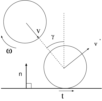
Figure 1: A schematic picture of collision between a sphere and a flat wall.

The impact process is important in granular physics. Although we believe that the static interaction among contact grains can be described by the contact mechanics of elastic materials, we little know the dynamical part of contact mechanics. Thus, the distinct element method which is the most popular method for the simulation of grains contains many unknown parameters.Cundall and Strack (1979) Therefore, the theory of impact for elastic materials gives the basis of granular physics.Jaeger et al. (1996); Kadanoff (1999); de Gennes (1999)

While $e$ has been believed to be less than $1$ in most situations, we have recently recognized that $e$ can exceed $1$ in oblique impactsSmith and Liu (1992); Calsamiglia et al. (1997); Louge and Adams (2002). In particular, Louge and AdamsLouge and Adams (2002) reported that $e$ increases as a linear function of the magnitude of $\tan\gamma$ in the oblique impact of a hard aluminum oxide sphere on a thick plate with the incident angle $\gamma$. In this case, Young’s modulus of the wall is $100$ times smaller than that of the sphere in the experiment. Thus, the physics of impact is one of interesting subjects in current statistical mechanics.

The organization of this paper is as follows. In the next section, we explain the current understanding of normal impacts including the quasi-static theory, the effect of radiation of sounds, and the effect of the plastic deformation. In section III, we summarize the standard treatments for oblique impacts which include Walton’s argumentWalton (1992); Walton and Braun (1986) and the theory by Maw et al.Maw et al. (1976) In section IV, we will introduce three typical approaches for simulation of impacts of elastic materials. In section V, we briefly explain the recent analysis to explain the anomalous behavior of the restitution coefficient exceeds unity. Section VI is the short summary of this paper.

II The current understanding on normal impact

This section is devoted to summarize the current understanding on a normal head-on collision of elastic spheres or a collision between a sphere and a wall. From the quasi-static theoryKuwabara and Kono (1987); Brilliantov et al. (1996); Morgado and Oppenheim (1997); Schwager and Pöschel (1998); Ramírez et al. (1999), we believe that the restitution coefficient $e$ decays as $1-e\propto v^{1/5}$ with $v=v_{n}$ for small impact velocity. The agreement between the theory and experimental results is fair.Kuwabara and Kono (1987); Sondergaard et al. (1990); Labous et al. (1997) For high speed impacts, the plastic deformation of elastic particles is dominant mechanism to determine the post-collisional processes. Experimental results support the theoretical prediction $e\propto v^{-1/4}$.Johnson (1972, 1985) At present, we do not have any appropriate theory for the finite impact speed but below the threshold at which plastic deformation takes place.

II.1 Mechanism of inelastic collision

Inelasticity arises from the transfer of translational kinetic energy to internal degrees of freedom. The dominant dissipative processes for low speed impacts are viscous effects of elastic materials, the heat conduction and the sound emission into or out of the elastic materials. When a local deformation with finite speed takes place in a macroscopic material, the system is excited to a nonequilibrium state and after that it is relaxed to an equilibrium state. It is not easy to specify the microscopic origin of viscous effects or the relaxation process, because such systems have numerous number of degree of freedom. However, at least, inelastic scatterings of phonons and excitation-radiation processes in electronic states are two major sources of the dissipations.

It should be noted that the coefficient of restitution of one-dimensional rods is insensitive to the impact speed but depends on the ratio of lengths for two colliding rods.Goldsmith (1960); Giese and Zippelius (1996); Aspelmeier et al. (1998) On the other hand, the restitution coefficient strongly depends on the impact speed and Poisson’s ratio in higher dimensional impacts. For example, the two-dimensional simulation by Gerl and ZippeliusGerl and Zippelius (1999) shows that inelasticity increases as Poisson’s ratio increases.

II.2 Outline of theory of a quasi-static impact

In this subsection, we present the outline of quasi-static theory for a normal impact of elastic spheres.

The theory is based on the contact theory of elastic spheres developed by Hertz.Hertz (1882) Hertzian contact theory predicts that the radius of contact $a$ and the elastic compress force $F_{el}$ for two spheres with radii $R$ and $R^{\prime}$ are respectively given by

$$a=F_{el}^{1/3}\left(D\frac{RR^{\prime}}{R+R^{\prime}}\right)^{1/3}:\quad F_{el}=\frac{h^{3/2}}{D}\left(\frac{RR^{\prime}}{R+R^{\prime}}\right)^{1/2}$$ (4)

where $h$ is the length of compression, and $D=\frac{3}{4}(\frac{1-\nu}{E}+\frac{1-\nu^{\prime 2}}{E^{\prime}})$ with Young’s modulus $E,E^{\prime}$ and Poisson’s ratio $\nu,\nu^{\prime}$ for two contact materials.Love (1927); Landau and Lifshitz (1960); Hills et al. (1993); Galin (1953); Johnson (1985)

Let us consider a low speed impact of two spheres. In the limit of low speed, the nonequilibrium processes may be suppressed, and the collision can be treated as an elastic process. The energy conservation can be read

$$m_{eff}\left(\frac{dh}{dt}\right)^{2}+\kappa h^{5/2}=m_{eff}v^{2},\quad\kappa=\frac{4}{5D}\displaystyle\sqrt{\frac{RR^{\prime}}{R+R^{\prime}}},$$ (5)

where $m_{eff}=mm^{\prime}/(m+m^{\prime})$ is the reduced mass of two spheres with masses $m$ and $m^{\prime}$. The maximum deformation is easily obtained as $h_{0}=(m_{eff}/\kappa)^{2/5}v^{4/5}$. The contact time $t_{c}$ of the collision which is two times as large as the time needed to reach $h_{0}$ is given by

$$t_{c}=2\left(\frac{m_{eff}^{2}}{\kappa^{2}v}\right)^{1/5}\int_{0}^{1}\frac{dx}{\sqrt{1-x^{5/2}}}=c_{t}\left(\frac{m_{eff}^{2}}{\kappa^{2}v}\right)^{1/5}$$ (6)

where $c_{t}=4\sqrt{\pi}\Gamma(2/5)/5\Gamma(9/10)\simeq 2.94$ with the Gamma function $\Gamma(x)$.

The above treatment predicts $e=1$, because the process does not contain any dissipation. Kuwabara and KonoKuwabara and Kono (1987) assume the existence of Rayleigh’s dissipation function for elastic solids, and write down the dissipative force as

$$F_{f}=-2\displaystyle\sqrt{\frac{RR^{\prime}}{R+R^{\prime}}}\frac{\sqrt{h}}{\tilde{D}}\frac{dh}{dt}$$ (7)

for two contacted spheres. Here, $\tilde{D}$ corresponds to $D$ for elastic contact, which can be represented by viscous parameters of Rayleigh’s dissipation function. The magnitude of the viscous parameter $\tilde{D}$ can be measured from an experiment of sound attenuation. Adding this viscous term, the dimensionless form of equation of motion becomes

$$\ddot{x}+\eta\sqrt{x}\dot{x}+\frac{5}{4}x^{3/2}=0;\quad\eta\equiv\frac{5}{2}\tilde{\kappa}\left(\frac{v}{\kappa^{3}m_{eff}^{2}}\right)^{1/5}$$ (8)

where $\tilde{\kappa}=(4/5\tilde{D})\sqrt{RR^{\prime}/(R+R^{\prime})}$. Here, we nondimensionalize the variables in terms of $h=h_{0}x$, $t=(h_{0}/v)\tau$, and thus $\dot{x}=dx/d\tau$. Thus, the problem is reduced to obtaining $e=dx/d\tau$ at $\tau_{c}=t_{c}(v/h_{0})$ under the initial conditions $x=0$ and $\dot{x}=1$. From (8), it is easy to obtain

$$e^{2}-1=-2\eta\int_{0}^{\tau_{c}}\sqrt{x}{\dot{x}}^{2}d\tau.$$ (9)

Since the exact evaluation of the integral is impossible, we may replace $x$ in the above equation by the solution of elastic equation. Using this approximation we obtain

$$e\simeq 1-1.009\eta=1-1.009\times\frac{5}{2}\tilde{\kappa}\left(\frac{v}{\kappa^{3}{m_{eff}}^{2}}\right)^{1/5},$$ (10)

where the numerical constant comes from $(4/5)B(3/5,3/2)\simeq 1.009$ with the beta function $B(x,y)$. Thus, the coefficient of restitution for the low speed impact is believed to decay $1-e\propto v^{1/5}$. The result can be obtained in different contexts.Morgado and Oppenheim (1997); Brilliantov et al. (1996)

Here, we briefly summarize the two-dimensional counterpart of normal impacts. For impacts of an elastic disk on a rigid wall, we do not have reliable argument. The total force of elastic force and dissipative force may be given by

$$F_{tot}\simeq-\frac{\pi E_{*}h}{\ln(4R/h)}-\tau_{0}\frac{\pi E_{*}\dot{h}}{\ln(4R/h)},$$ (11)

where $E_{*}=E/(1-\nu^{2})$ and $\tau_{0}$ represents the time scale for the dissipation of the small deformation. Replacing the logarithmic term as a constant correction, the equation for elastic motion can be solved. Thus, we may evaluate the contact time $t_{c}$ as

$$t_{c}\simeq\frac{\pi R}{c}\displaystyle\sqrt{\ln\frac{4c}{v}}$$ (12)

where $c=\sqrt{E_{*}/\rho}$ and $\rho$ are the compressive sound velocity and the density, respectively.Gerl and Zippelius (1999); Hayakawa and Kuninaka (2002) From the comparison of eq.(12) with a two-dimensional simulation, we have confirmed that the above estimation is quantitatively correct.Hayakawa and Kuninaka (2002) Here, we adopt a bold approximation: $h_{max}\simeq vR\sqrt{(\rho/E_{*})\ln(4R/h)}\sim vR/c$. Including the dissipative force this approximation gives

$$e\simeq 1-\frac{2\pi E_{*}}{\rho Rc\sqrt{\ln(4c/v)}}.$$ (13)

The correctness of this expression has not been confirmed.

II.3 The effect of radiation of elastic waves

So far, we do not have any theoretical argument to estimate the restitution coefficient as a result of radiation of elastic waves. On the other hand, Miller and PurseyMiller and Pursey (1954, 1955) calculated the averaged power radiated per unit area by the normal oscillating contact of circular region on a semi-infinite isotropic elastic material. Although the situation is a little different each other, we may apply their calculation to estimate the energy loss by radiation of elastic waves.

Miller and PurseyMiller and Pursey (1954, 1955) obtained the powers radiated in the compressible ($W_{c}$) and shear waves ($W_{s}$) as

$$W_{c} = \frac{a^{4}{k_{1}}^{2}t_{c}\zeta^{4}P_{0}^{2}}{4\rho}\int_{0}^{\pi/2}d\theta\{\Theta_{1}(\theta)\}^{2}\sin\theta$$ (14)

$$W_{s} = \frac{a^{4}{k_{1}}^{2}t_{c}\zeta^{9}P_{0}^{2}}{4\rho}\int_{0}^{\pi/2}d\theta|\Theta_{2}(\theta)|^{2}\sin\theta,$$ (15)

where $\theta$ is the polar angle from the axis of symmetry, $P_{0}=F_{el}/(\pi a^{2})$ is the average compressive force, and

$$\Theta_{1}(\theta) = \frac{\cos\theta(\zeta^{2}-2\sin^{2}\theta)}{F_{0}(\sin\theta)}\quad\Theta_{2}(\theta)=\frac{\sin 2\theta\sqrt{\zeta^{2}\sin^{2}\theta-1}}{F_{0}(\zeta\sin\theta)}$$ (16)

$$F_{0}(x) \equiv (2x^{2}-\zeta^{2})^{2}-4x^{2}\sqrt{(x^{2}-\zeta^{2})(x^{2}-1)},$$ (17)

$$k_{1} = \frac{\pi}{t_{c}}\sqrt{\frac{\rho(1+\nu)(1-2\nu)}{E(1-\nu)}},\quad k_{2}=\frac{\pi}{t_{c}}\sqrt{\frac{2\rho(1+\nu)}{E}}$$ (18)

$$\zeta = k_{2}/k_{1}=\sqrt{\frac{2(1-\nu)}{1-2\nu}}.$$ (19)

Here we omit the power radiated in terms of surface waves which plays an important role in the paper by Miller and PurseyMiller and Pursey (1954, 1955), because they can be absorbed as the numerical factor and the treatment for spherical surfaces is not obvious. The integrations of $W_{c}$ and $W_{s}$ are possible once we specify the material. For example, in the case of the material with $\nu=1/4$, i.e. $\zeta=\sqrt{3}$, the total amount of power is given by

$$W=W_{c}+W_{s}=1.579\frac{a^{4}{k_{1}}^{2}t_{c}\zeta^{4}P_{0}^{2}}{4\rho}.$$ (20)

The energy loss during collision is thus given by

$$E_{loss}=2\int_{0}^{t_{c}/2}dtW\simeq\frac{5.337}{\rho t_{c}^{2}E^{3/2}}\int_{0}^{t_{c}/2}dtF_{el}^{2}.$$ (21)

Similarly the argument in the previous section, the integral in the right hand side can be evaluated as $\int_{0}^{t_{c}/2}dtF_{el}^{2}=5\sqrt{\pi}\Gamma(8/5)/(8\Gamma(21/10))\kappa^{2/5}m_{eff}^{8/5}v^{11/5}$ in the elastic limit. Thus, we obtain

$$E_{loss}\simeq 0.5827\frac{\kappa^{6/5}m_{eff}^{4/5}}{\rho E^{3/2}}v^{13/5}.$$ (22)

From the relation $E_{loss}=(1-e^{2})m_{eff}v^{2}/2\simeq m_{eff}v^{2}(1-e)$, we finally reach the new relation:

$$1-e\simeq 0.5827\frac{\kappa^{6/5}}{\rho m_{eff}^{1/5}E^{3/2}}v^{1/5},$$ (23)

for $\nu=1/4$. The discussion here is the rough evaluation of the restitution coefficient based on the energy loss by radiation of elastic waves. Although the numerical constant in eq.(23) is meaningless, we expect that the scaling relation can be used in realistic situations. It is interesting that the restitution coefficient $e$ obeys $1-e\propto v^{1/5}$ which is the essentially same as that of the quasi-static theory.Kuwabara and Kono (1987); Morgado and Oppenheim (1997); Brilliantov et al. (1996); Schwager and Pöschel (1998); Ramírez et al. (1999)

It should be noted that HunterHunter (1957) derived $1-e\propto v^{3/5}$ from the theory of Miller and Pursey.Miller and Pursey (1954, 1955) The difference comes from the followings. HunterHunter (1957) assumes that the energy dissipation is obtained from

$$W_{H}=\int_{0}^{t_{c}}dt\pi a^{2}F_{el}(t)\frac{d\bar{u}(t)}{dt},$$ (24)

where $\bar{u}(t)$ is the mean surface displacement. Although HunterHunter (1957) adopts the result of Miller and PurseyMiller and Pursey (1954, 1955) for $\bar{u}$, this is only the fraction of the radiation. The above treatment presented here is more reliable.

However, the analysis presented in this subsection is still prematured. Insufficient parts of the analysis are as follows: (i) The theory by Miller and PurseyMiller and Pursey (1954, 1955) assume the constant pressure in the contact area, but Hertzian contact theory predicts the distribution of pressure. (ii) Miller and PurseyMiller and Pursey (1954, 1955) discussed the radiation of elastic wave for semi-infinitely large region, but the actual contacted spheres have curvature and finite volume. Therefore, we may need more systematic treatment for the radiation of elastic waves.

II.4 Impact with plastic deformation

When the impact speed is large enough, the elastic description is no longer valid but we have to consider the effects of plastic deformation. The restitution coefficient drastically decreases when the plastic deformation occurs. Following the argument by JohnsonJohnson (1985), we review the argument of the restitution coefficient for impacts with plastic deformations. In the argument in this subsection, we neglect numerical factors. So the result is basically valid for collisions for two spheres with equal radius $R$ and the density.

Let us evaluate the yield pressure. From Hertzian contact theory the maximum pressure of compression exists at the center of contact and its expression is given by

$$p_{0}=\frac{3F_{el}}{2\pi a^{2}}=\left(\frac{6F_{el}{E_{*}}^{2}}{\pi^{3}R^{2}}\right)^{1/3}.$$ (25)

Thus, the compressive elastic force at the yield pressure $p_{0}=(p_{0})_{Y}$ becomes

$$F_{el}=\frac{\pi^{3}R^{2}}{6{E_{*}}^{2}}(p_{0})_{Y}^{3},$$ (26)

where $(p_{0})_{Y}$ is about 1.6 $E$ at Mises’ condition.Johnson (1985)

Hertzian contact theory gives $F_{el}\sim E_{*}R^{1/2}h^{3/2}$, while the maximum deformation is

$$h_{*}\sim\left(\frac{mv^{2}}{R^{1/2}E_{*}}\right)^{2/5}$$ (27)

from $mv^{2}\sim F_{el}h\sim E_{*}R^{1/2}h^{5/2}$, where $m$ is the mass of each sphere. Substituting this $h_{*}$ into Hertzian contact theory with setting $F_{el}=F_{Y}$, we balance the force with $F_{Y}\sim\frac{R^{2}}{{E_{*}}^{2}}(p_{0})_{Y}^{3}$. Then we obtain

$$(p_{0})_{Y}\sim\left(\frac{E_{*}}{R^{3/4}}\right)^{4/5}(mv^{2})^{1/5},$$ (28)

which is the condition for yield stress.

Let us discuss the effect of plastic deformation to the restitution coefficient. From Hertzian contact theory there is a relation between the compression and the radius of the contact $h\sim a^{2}/R$. Therefore the deformation $h_{*}$ for the plastic deformation becomes $h_{*}\sim F_{*}/(E_{*}a_{*})$ because of $F_{*}\sim E_{*}\sqrt{Rh}h$, where $a_{*}$ and $F_{*}$ are respectively the radius of contact area and the compressive force for the plastic deformation. Thus, the internal energy stored during the deformation may be evaluated as $W^{\prime}\sim F_{*}h_{*}\sim{F_{*}}^{2}/(a_{*}E_{*})$. On the other hand, we have $F_{*}=\pi a_{*}^{2}p_{d}$ with the contact pressure $p_{d}$. Since the stored energy is released as the kinetic energy in impact processes, the kinetic energy for rebound is given by $K_{r}\sim W^{\prime}\sim a_{*}^{3}p_{d}^{2}/E_{*}$.

On the other hand, we can estimate the work needed for compression as $W=(1/2)mv^{2}\sim\int_{0}^{h_{*}}dhF_{el}\sim\int_{0}^{a_{*}}daF_{*}a/R$. Assuming that $F_{el}=\pi a^{2}p_{d}$ is kept during the impact, we obtain

$$W=\int_{0}^{a_{*}}\frac{\pi p_{d}a^{3}da}{R}\sim\frac{p_{d}{a_{*}}^{4}}{R}\sim mv^{2}.$$ (29)

Thus, we reach

$$e^{2}=\frac{{v^{\prime}}^{2}}{v^{2}}\sim\frac{p_{d}R}{E_{*}a_{*}}.$$ (30)

Equation (30) can be rewritten as

$$e^{2}\sim\frac{p_{d}}{E_{*}}\left(\frac{p_{d}R^{3}}{mv^{2}}\right)^{1/4}$$ (31)

and thus, we finally obtain

$$e\propto v^{-1/4}.$$ (32)

This expression recovers experimental results.

III Current Understanding of Oblique Impact

III.1 Walton’s argument

To characterize the oblique collision, Walton introduced three parameters:Walton (1992); Walton and Braun (1986) the coefficient of normal restitution $e$, the coefficient of Coulomb’s friction $\mu$, and the maximum value of the coefficient of tangential restitution $\beta_{0}$. The expression is given by

$$\beta\simeq\left\{\begin{array}[]{ll}-1-\mu(1+e)\cot\gamma\left(1+\frac{mR^{2}}{I}\right)&\quad(\gamma\geq\gamma_{0})\\ \beta_{0}&\quad(\gamma\leq\gamma_{0}),\end{array}\right.$$ (33)

where $\gamma_{0}$ is the critical angle, and $m$, $R$, and $I$ are mass, radius and moment of inertia of spheres respectively.Walton (1992); Walton and Braun (1986) Experiments have supported that his characterization adequately capture the essence of binary collision of spheres or collision of a sphere on a flat plateLabous et al. (1997); Foerster et al. (1994); Lorentz et al. (1997); Gorham and Kharaz (2000).

The derivation of the first equation of Walton’s expression is simple. When there is a slip, the friction coefficient satisfies

$$|{\bf n}\times{\bf J}|=\mu({\bf n}\cdot{\bf J}),$$ (34)

where ${\bf J}=m({\bf v}^{\prime}-{\bf v})$ is the impulse. Let us write ${\bf J}$ as the following form:

$${\bf J}=A({\bf n}\cdot{\bf v}_{c}){\bf n}+B[{\bf v}_{c}-({\bf n}\cdot{\bf v}_{c}){\bf n}],$$ (35)

where $A$ and $B$ are constants to be determined. From the definition of $e$ and $\beta$ with the aid of $I({\mbox{\boldmath$\omega$}}^{\prime}-\mbox{\boldmath$\omega$})=-R({\bf n}\times{\bf J})$ we write

$$m({\bf v}_{c}^{\prime}-{\bf v}_{c})=A({\bf n}\cdot{\bf v}_{c}){\bf n}+(1+\frac{mR^{2}}{I})B[{\bf v}_{c}-({\bf n}\cdot{\bf v}_{c}){\bf n}].$$ (36)

Thus, from the projection to the normal direction we obtain $A=-m(1+e)$ and $B=(1+mR^{2}/I)m(1+\beta)$. On the other hand, through the relation $|{\bf n}\times{\bf J}|=B|{\bf n}\times{\bf v}_{c}|=\mu({\bf n}\cdot{\bf J})=\mu A({\bf n}\cdot{\bf v}_{c})$, we can rewrite ${\bf J}$ as

$${\bf J}=-m(1+e)({\bf n}\cdot{\bf v}_{c}){\bf n}+\mu m(1+e)\cot\gamma[{\bf v}_{c}-({\bf n}\cdot{\bf v}_{c}){\bf n}].$$ (37)

Thus, we obtain the first expression of eq.(33).

Figure 2: Comparison between Walton’s argument and our numerical result. Here $\Psi_{1}=\tan\gamma$ and $\Psi_{2}=-{v_{t}}^{\prime}/v_{n}$. Parameters for the simulation are the same as those in ref.Kuninaka and Hayakawa (2003).

In spite of its simple form and its simple derivation, Walton’s expression is useful to characterize oblique impacts. However, we do not know how to determine $\beta_{0}$ and $\gamma_{0}$. In addition, it cannot be applied to impacts for very small $\gamma$ in which $\beta$ cannot be a constant, because it should not be contradict with the normal impact at $\gamma=0$. The discontinuity of differentiation of $\beta$ at $\gamma=\gamma_{0}$ is also unnatural. To know the details of physics of the oblique impacts we should introduce alternative theory.

III.2 Theory of Maw et al.

More systematic treatment for oblique impacts is developed by Maw et al.Maw et al. (1976); Stronge (2000); Kuninaka and Hayakawa (2003) The complete explanation of their theory is long because of its complicated structure. Here, we only summarize the result of the theory.

They assume that the stiffness of normal compliance for restitution changes from $k$ to $k/e^{2}$ where $k$ is the normal stiffness for compression. They do not discuss the origin of the normal restitution coefficient $e$ which is assumed to be constant and its effect for the stiffness explicitly.

They also indicate that there are three region depending on the incident angle $\gamma$. According to their theoryMaw et al. (1976), $\beta$ for the impact of a circular disk on a wall can be represented byKuninaka and Hayakawa (2003)

1. $1/\mu\sigma^{2}<\cot\gamma$ with $\sigma=\sqrt{(2-\nu)/(2(1-\nu))}$:

   $$\beta=-\cos\omega t_{1}-\mu\frac{\beta_{x}}{\beta_{z}}e\left[1+\cos\left(\frac{\Omega t_{1}}{e}+\frac{\pi}{2}(1-e^{-1})\right)\right]\cot\gamma,$$ (38)

2. $\beta_{x}/\beta_{z}\mu(1+e)<\cot\gamma<1/\mu\sigma^{2}$:

   $$\beta = -\cos\omega(t_{3}-t_{2})-\mu\frac{\beta_{x}}{\beta_{z}}[\cos\omega(t_{3}-t_{2})-\cos\Omega t_{2}\cos\omega(t_{3}-t_{2})$$ (39)

   $$+\frac{\Omega}{\omega}\sin\Omega t_{2}\sin\omega(t_{3}-t_{2})+e+\cos\Omega t_{3}]\cot\gamma,$$

3. $\cot\gamma<\beta_{x}/\beta_{z}\mu(1+e)$:

   $$\beta=-1+\mu\frac{\beta_{x}}{\beta_{z}}\left(1+e\right)\cot\gamma,$$ (40)

where $\mu$ is the coefficient of friction, $\beta_{x}=3$ and $\beta_{z}=1$ are constants for the impact of the disk on the infinite wall. $\Omega$ and $\omega$ are respectively $\pi/2t_{0}$ and $(\pi/2\sigma t_{0})\sqrt{\beta_{x}/\beta_{z}}$, where $t_{0}$ is the time for compression. The time $t_{1}$ is the transition time from initial stick motion to slip motion which is determined by

$$\frac{|F_{x}(t_{1})|}{\mu F_{z}(t_{1})}=\left\{\begin{array}[]{ll}\displaystyle\frac{1}{\sigma^{2}}\frac{v_{x}(0)}{\mu v_{z}(0)}\frac{\Omega}{\omega}\frac{\sin\omega t_{1}}{\sin\Omega t_{1}}=1&0\leq t_{1}<t_{0}\\ \displaystyle\frac{1}{\sigma^{2}}\frac{v_{x}(0)}{\mu v_{z}(0)}\frac{\Omega}{\omega}\frac{\sin\omega t_{1}}{\sin(\frac{\Omega t_{1}}{e}+\frac{\pi}{2}(1-e^{-1}))}=1&t_{0}\leq t_{1}<t_{f},\end{array}\right.$$ (41)

where $v_{x}(t)$ and $v_{z}(t)$ are the tangential and the normal relative velocities at the contact point, respectively. While $t_{2}$ can be determined by (42) :

$$\begin{array}[]{lr}\Omega t_{2}=\arccos\left(\displaystyle\frac{v_{x}(0)/\mu v_{z}(0)-\beta_{x}/\beta_{z}}{\sigma^{2}-\beta_{x}/\beta_{z}}\right)&{\rm for}{~{}}\displaystyle\frac{v_{x}(0)}{v_{z}(0)}\leq\mu\displaystyle\frac{\beta_{x}}{\beta_{z}}\\ \displaystyle\frac{\Omega t_{2}}{e}=-\displaystyle\frac{\pi}{2}(1-e^{-1})+\arccos\left(\frac{v_{x}(0)/\mu v_{z}(0)-\beta_{x}/\beta_{z}}{\sigma^{2}e^{-1}-e\beta_{x}/\beta_{z}}\right)&{\rm for}{~{}}\displaystyle\frac{v_{x}(0)}{v_{z}(0)}>\mu\displaystyle\frac{\beta_{x}}{\beta_{z}}\end{array}$$ (42)

which is the time to start sticking. The time $t_{3}$ determined by solving eqs.(43) numerically is the transition time from stick motion to slip motion:

$$\left|\frac{\Omega u_{x}(t_{2})}{\mu v_{z}(0)}\cos\omega(t_{3}-t_{2})-\frac{\Omega v_{x}(t_{2})}{\omega\mu v_{z}(0)}\sin\omega(t_{3}-t_{2})\right|=\sigma^{2}\sin\left[\frac{\Omega t_{3}}{e}+\frac{\pi}{2}(1-e^{-1})\right],$$ (43)

where $u_{x}(t_{2})$ is the tangential deformation at time $t_{2}$. By calculating $\beta$ at each value of $\cot\gamma$ and interpolating them with cubic spline interpolation method, we can draw the theoretical curve.

Figure 3: Comparison between Maw’s theory and our numerical result. The situation is the same as that in ref.Kuninaka and Hayakawa (2003).

Figure 3 shows comparison of the theory with our numerical simulation, in which the agreement is acceptable.

As is shown, the theory by Maw et al.Maw et al. (1976); Stronge (2000) captures the physics of impact processes. For large $\gamma$, i.e. region (iii), the disk slips on the wall without any rotation or sticking. For intermediate $\gamma$, that is, the region (ii), the disk slips at first and stick at $t=t_{2}$ and slips again at $t=t_{3}$. For small $\gamma$ in the region (i), the disk sticks initially and begins to slip at $t=t_{1}$. In this sense, their theory improves some defects of Walton’s argument.Walton (1992); Walton and Braun (1986) However, their theory includes some other defects: The final expression for $\beta$ is complicated and is required for numerical calculation. It still contains undetermined parameters $e$ and $\mu$ which are assumed to be constants. As is shown, $e$ and $\mu$ strongly depend on the impact speed and the incident angle.Kuwabara and Kono (1987); Morgado and Oppenheim (1997); Brilliantov et al. (1996); Sondergaard et al. (1990); Labous et al. (1997); Vincent (1900); Schwager and Pöschel (1998); Ramírez et al. (1999); Gerl and Zippelius (1999); Hayakawa and Kuninaka (2002); Gorham and Kharaz (2000); Louge and Adams (2002); Kuninaka and Hayakawa Thus, we cannot justify their assumption.

IV Numerical modeling

In general, the success of theoretical approach is limited for nonlinear problems because of difficulties of analysis. On the other hand, numerical approach has become standard as computers become popular. The advantage of this approach is obvious. (i) We can investigate collision processes under idealistic situations. (ii) It is easy to control situations to investigate the properties of impact processes. (iii) It is possible to analyze nonlinear problems. However, when we restrict our interest in numerical studies of impacts, we still do not have any standard technique and the status of such the studies is prematured.

One of typical approaches for engineers is to use FEM (Finite Element Method).Smith and Liu (1992); Lim and Stronge (1998, 1999); Minamoto and Takezono (2003); Wu et al. (2003) There are some standard packages for simulation of impact processes. For example, Lim and StrongeLim and Stronge (1998, 1999) carried out two-dimensional simulation of a transverse collision of a cylinder against an elastoplastic half space based on DYNA2D. A three-dimensional FEM also exists.Minamoto and Takezono (2003) All of them reproduce experimental results. Since FEM is originally proposed for a solver for static problems, they can recover the Hertzian contact theory for the static elastic problem. No viscous term, however, is included within FEM. To obtain inelastic impacts, FEM usually introduces elastic-plastic deformation or fully plastic deformation. Therefore, the simulation based on FEM sometimes predicts $e\propto v^{-1/4}$ without quasi-static region.Lim and Stronge (1998) We also note that there are many input parameters for FEM. For example, it includes at least two yield stresses for the transition from the elastic region to the elastic-plastic region, and the transition from the elastic-plastic region to the fully plastic region. It also contains at least two friction coefficient as a constant. However, as will be shown, the friction coefficient cannot be regarded as a constant.

Another approach is proposed by Gerl and ZippeliusGerl and Zippelius (1999); Hayakawa and Kuninaka (2002) which is based on the mode analysis of elastic materials. They assume that an isolated disk is in an eigenstate of isothermal vibration of elastic waves. When the disk contacts a wall, the transitions among eigenstates is induced by nonlinear effects of interaction between the disk and the wall.

The last approach is based on the equation of motion for mass points connected by springs.Hayakawa and Kuninaka (2002); Kuninaka and Hayakawa (2003) This approach is intuitive and flexible. For example, the other approaches may not be applied to impacts with rough surfaces without essential change of algorithms, but this approach can include the roughness at surface easily. The roughness at surface plays crucial roles for oblique impacts. In fact, the coefficient of tangential restitution $\beta$ becomes -1 without the roughness.Kuninaka and Hayakawa (2003) The disadvantage of this approach is that the code is not fast, and the result strongly depends on lattice structures.

The last two approaches are adequate for the high speed impact without plastic deformation. At present, there is no three dimensional simulations, and two-dimensional simulations for normal impacts may not agree with those for quasi-static theory. One of defects for these approaches is that the problem is not relaxed to a static state without introduction of local dissipation. For later discussion, we focus on the last approach to simulate the oblique impact of a disk on a flat wall to clarify the mechanism of anomalous behavior of the restitution coefficient $e$.

V Simulation of oblique impact

Figure 4: The elastic disk and wall consisted of random lattice.

V.1 Our model

Let us introduce our numerical modelKuninaka and Hayakawa (2003, ) which is a typical example of the last approach in the previous section. The discussion in this section is based on our recent paper.Kuninaka and Hayakawa

Our numerical model consists of an elastic disk and an elastic wall (Fig. 4). The width and the height of the wall are $8R$ and $2R$, respectively, where $R$ is the radius of the disk. We adopt the fixed boundary condition for the both side ends and the bottom of the wall. To make each of them, at first, we place mass points at random in a circle and a rectangle with the same density, respectively. For the disk, we place $800$ particles at random in a circle with the radius $R$ while for the wall, similarly, we place $4000$ particles at random in a rectangle.

After that, we connect all mass points with nonlinear springs for each of them using the Delaunay triangulation algorithmSugihara (2001). The spring interaction between connected mass points is given by

$$V^{(i)}(x)=\frac{1}{2}k^{(i)}_{a}x^{2}+\frac{1}{4}k^{(i)}_{b}x^{4},\hskip 8.53581pti=d\text{(disk)},w\text{(wall)},$$ (44)

where $x$ is a stretch from the natural length of spring, and $k^{(i)}_{a}$ and $k^{(i)}_{b}$ are the spring constants for the disk($i$=d) and the wall($i$=w).

In most of our simulations, we adopt $k^{(d)}_{a}=1.0\times m_{0}c^{2}/R^{2}$for the disk while $k^{(w)}_{a}=k^{(d)}_{a}/100$ for the wall, where $m_{0}$ and $c$ are the mass of each mass point and the one-dimensional velocity of sound, respectively. In this model, the wall is much softer than the disk as in ref.Louge and Adams (2002). We adopt $k^{(i)}_{b}=k^{(i)}_{a}\times 10^{-3}/R^{2}$ for each of them. We do not introduce any dissipative mechanism in this model. The interaction between the disk and the wall during a collision is given by ${\bf F}(l)=\xi V_{0}\exp(\xi l){\bf n}^{s}$, where $\xi$ is $300/R$, $V_{0}$ is $\xi m_{0}c^{2}R/2$, $l$ is the distance between each surface particle of the disk and the surface spring of the wall, and ${\bf n}^{s}$ is the normal unit vector to the spring.

In this model, the roughness of the surfaces is important to make the disk rotate after collisionsKuninaka and Hayakawa (2003). To make roughness, the normal random numbers with its average is zero and its standard deviation is $\delta=3\times 10^{-2}R$ are used for the surface particles of the disk and the wall. All the data in this paper are obtained from the average of 100 samples in random numbers.

Poisson’s ratio $\nu$ and Young’s modulus $E$ of this model can be evaluated from the strains of the band of random lattice in vertical and horizontal directions to the applied force. We obtain Poisson’s ratio $\nu$ and Young’s modulus $E$ as $\nu=(7.50\pm 0.11)\times 10^{-2}$ and $E=(9.54\pm 0.231)\times 10^{3}m_{0}c^{2}/R^{2}$, respectively.Kuninaka and Hayakawa (2003)

In our simulation, we define the incident angle $\gamma$ by the angle between the normal vector of the wall and the initial velocity vector of the disk(see Fig. 4). We fix the initial colliding speed of the disk as $|{\bf v}(0)|=0.1c$ to control the normal and tangential components of the initial colliding velocity as $v_{t}(0)=|{\bf v}(0)|\sin\gamma$ and $v_{n}(0)=|{\bf v}(0)|\cos\gamma$, respectively. We use the fourth order symplectic numerical method for the numerical scheme of integration with the time step $\Delta t=10^{-3}R/c$.

Figure 5: Numerical and theoretical results of the relation between $\Psi_{1}$ and $e$.

V.2 Results

Figure 5 is the normal restitution coefficient $e$ against $\Psi_{1}=\tan\gamma$ for the impact of the hard disk on the soft wall. The cross points are the average and the error bars are the standard deviation of 100 samples for each incident angle. This result shows that $e$ increases as $\Psi_{1}$ increases to exceed unity, and has a peak around $\Psi_{1}=6.0$. This behavior is contrast to that in the experiment by Louge and AdamsLouge and Adams (2002).

Let us clarify the mechanism of our results. Louge and AdamsLouge and Adams (2002) suggest the anomalous behavior of $e\geq 1$ can be understood by the local deformation on the surface of the wall during an impact. They attribute their results to the rotation of normal unit vector of the wall surface by an angle $\alpha$ and derive the corrected expression for $e$. Thus, we determine the quantity of $\alpha$ at each incident angle from the theory of elasticity and calculate corrected $e$.

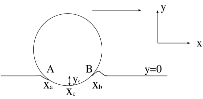
Figure 6: The schematic figure of a hard disk sliding on a soft wall. $x$ coordinates of both ends of the contact area AB are $x=x_{a}$ and $x=x_{b}$.

Figure 6 is the schematic figure of a hard disk moving from left to right on a wall, where the length of the contact area is $l=|x_{b}-x_{a}|$. From the theory of elasticityHills et al. (1993); Galin (1953), this ratio can be estimated as

$$\frac{x_{c}-x_{a}}{l}=1-\theta\hskip 14.22636pt\text{with}\hskip 14.22636pt\theta=\frac{1}{\pi}\arctan\frac{1-2\nu}{\mu(2-2\nu)},$$ (45)

where $\nu$ is Poisson’s ratio of the wall and $\mu$ is the coefficient of friction. Here $\tan\alpha\equiv\frac{f(x_{b})-f(x_{a})}{l}$ with the deformed shape of the wall $f(x)$ approximated by a parabolic function near $x_{c}$ is reduced to

$$\tan\alpha=\frac{1-2\theta}{2-2\theta}\frac{|x_{c}-x_{a}|}{R}.$$ (46)

In eq.(46), $|x_{c}-x_{a}|$ can be evaluated by the simulation data. From our simulation, the maximum value of $y_{c}$ is about $0.17R$ at $\Psi_{1}=1.0$. Assuming the disk is pressed in the normal direction, we can estimate the contact area as about $1.1R$ which is the maximum value. Thus, we adopt its half value, $0.55R$, as $|x_{c}-x_{a}|$.

The cross points in Fig.7 is $\mu$ calculated from eq.(34) and our simulation data against each $\Psi_{1}$. Figure 7 shows $\mu$ has a peak around $\Psi_{1}=3.0$. Substituting this result to eqs.(45) and (46), we obtain the relation between $\Psi_{1}$ and $\tan\alpha$.

The restitution coefficient $e$ can be obtained as a function of $\tan\alpha$ by regarding the impact as that on a tilted surface with the angle $\alpha$. Skipping the derivation, we can write the result asKuninaka and Hayakawa

$$e=\frac{e_{\alpha}+\Psi_{2}^{\alpha}\tan\alpha}{1-\Psi_{1}^{\alpha}\tan\alpha},$$ (47)

where $e_{\alpha}$ is the restitution coefficient defined through

$${\bf v_{c}}^{\prime}\cdot{\bf n}_{\alpha}=-e_{\alpha}({\bf v_{c}}\cdot{\bf n}_{\alpha}),$$ (48)

where ${\bf n}_{\alpha}$ is the unit normal vector of the tilted slope connecting $A$ and $B$ in Fig.6. Here $\Psi_{1}^{\alpha}$ and $\Psi_{2}^{\alpha}$ are respectively given by

$$\Psi_{1}^{\alpha}=\frac{\Psi_{1}-\tan\alpha}{1+\Psi_{1}\tan\alpha}.$$ (49)

and

$$\Psi_{2}^{\alpha}=\Psi_{1}^{\alpha}-3(1+e_{\alpha})\mu_{\alpha}$$ (50)

in the two-dimensional situationWalton (1992); Walton and Braun (1986). $\mu_{\alpha}$ in eq.(50) is given by

$$\mu_{\alpha}=\frac{\mu+\tan\alpha}{1-\mu\tan\alpha}.$$ (51)

To draw the solid line in Fig.5, at first, we calculate $\tan\alpha$ and $\mu$ by eqs.(46) and (34) respectively for each $\Psi_{1}$. After that, we calculate $\Psi_{1}^{\alpha}$ and $\Psi_{2}^{\alpha}$ by eqs.(49) and (50), and obtain $e$ by substituting them into eq.(47) for each $\Psi_{1}$. Although $e_{\alpha}$ is assumed to be a constant in ref.Kuninaka and Hayakawa , here we evaluate $e_{\alpha}$ from our simulation which has the weak dependence of $\gamma$. The solid line of Fig.5 is eq.(47). All points are interpolated with cubic spline interpolation method to draw the theoretical curve. Such the theoretical description of $e$ is consistent with our numerical result. As can be seen, the restitution coefficient $e$ depends on the relation between $\mu$ and $\Psi_{1}$.

Figure 7: Numerical and theoretical results of the relation between $\Psi_{1}$ and $\mu$.

It should be noted that the behavior of $\mu$ as a function of $\gamma$ can be understood by using a simple phenomenological argument. The solid curve in Fig.7 is the fitting curve obtained from the theory. If we omit the collapse of the roughness by the impact for large $\gamma$ close to $\pi/2$, both $\mu$ and $e$ increase with increasing $\gamma$. This suggests that the discrepancy between our result in Fig.5 and the result by Louge and AdamsLouge and Adams (2002) is originated from the difference of impact speed. Namely, our impact speed much larger than the experimental one. Although we skip the details of derivation, it may be clear that our argument captures the essence of physics of the oblique impact.

V.3 Discussion

At first, let us discuss the origin of the relation between $e$ and $\Psi_{1}$. As was indicated, the local deformation of the wall’s surface is essential for $e$ to exceed unity. We have also carried out the simulation when $k^{(w)}_{a}=10\times k^{(d)}_{a}$, which means the wall is harder than the disk. In this case, $e$ takes almost constant value to exceed unity suddenly around $\Psi_{1}=4.5$. This tendency resembles the experiment by Calsamiglia et al.Calsamiglia et al. (1997). This behavior can be understood as that the disk is scattered by hard nails distributed on the surface of the wall.

Figure 8: Numerical results of $e$ for the impact of a soft disk on a hard wall. It should be noted that $\Psi_{1}=4.5$ is almost the same as the largest $\gamma$ in the experiment of ref.Calsamiglia et al. (1997).

Thus, the wall should be much softer than the disk to get smooth increases of $e$ as increasing $\gamma$. In addition, it is important to fix the initial kinetic energy of the disk. We have confirmed so far that $e$ cannot exceed unity when we change $\gamma$ with fixed $v_{n}$Kuninaka and Hayakawa (2003).

Second, the initial velocity of the disk and the local deformation of the wall are so large that the local dissipation in springs and the gravity have not affected our numerical results. In addition, we have carried out the other simulation with a disk of $400$ particles and a wall of $2000$ particles to investigate the effect of the model size. Although there is a slight difference between the results, the data can be reproduced quite well by our phenomenological theory.

Third, the local deformation of the wall also affects the relation between $\mu$ and $\Psi_{1}$. In early studies, it has been shown that $\mu$ depends on the impact velocity Gorham and Kharaz (2000); Louge and Adams (2002). In our simulation, the magnitude of $\alpha$ has a peak around $\Psi_{1}=3.0$. This behavior is interpreted as that the local deformation collapses for large $v_{t}$. The decrease of $\mu$ and the friction force cause the decrease of $e$.

In final, we adopt the static theory of elasticity to explain our numerical results for the discussion here. However, it is important to solve the time-dependent equation of the deformation of the wall surface to analyze the dynamics of impact phenomena. The dynamical analysis is our future task.

In summary of this section, we have carried out the two-dimensional simulation of the oblique impact of an elastic disk on an elastic wall. We have found that the restitution coefficient $e$ can exceed unity in the oblique impact, which is attributed to the local deformation of the wall. The relation between $\mu$ and $\Psi_{1}$ is also related to the local deformation and can be explained by a simple theory.

VI Summary

We review the current understanding on inelastic impacts of elastic materials. We explain the standard theories for the normal impact and for oblique impacts. We also introduce some typical approaches for numerical simulation for impact problems. Although this problem is fundamental and familiar in elementary mechanics, the theoretical treatment is prematured. In recent finding of the anomalous behavior of the restitution coefficient exceeds unity is an example to have potential to be developed as a subject of physics. Unfortunately, most of the existing theories are based on engineering idea and they are not so simple and beautiful. In some cases, the assumption of the theory may not be valid. For physicists, in other words, there will be a lot of room for improvement of the theory of impact of elastic materials.