Dynamics of correlations in atomic Bose-Einstein condensates

Abstract

The Gross-Pitaevskii equation has been extremely successful in the theory of weakly-interacting Bose-Einstein condensates. However, present-day experiments reach beyond the regime of its validity due to the significant role of correlations. We review a method of tackling the dynamics of correlations in Bose condensed gases, in terms of noncommutative cumulants. This new approach has a wide range of applicability in the areas of current interest, e.g. the production of molecules and the manipulation of interactions in condensates. It also offers an interesting perspective on the classical-field methods for partly condensed Bose gases.

Eight years after the first experimental achievement of Bose-Einstein condensation of atoms Anderson95 , the field of quantum-degenerate gases is not losing its pace. On the contrary, it continues to open new and promising avenues for research, with the latest hot topics including quantum vortices Matthews99 ; Madison00 , Bose condensation of molecules Jochim03 and prospects of elucidating pairing mechanisms with the help of ultracold Fermi gases Levi03 .

Given the enormous potential and diversity of the field, it comes as a surprise that most of the experiments performed so far with Bose-Einstein condensates have been modelled almost perfectly by mean-field theory. The famous Gross-Pitaevskii equation Pitaevskii61 ; Gross61 has proved to be a genuine workhorse in the area, being employed in a myriad of contexts Dalfovo99 . An interesting and relatively new addition to the plethora of applications is a classical-field method for the dynamics of interacting Bose gases at non-zero temperatures Svistunov91 ; Damle96 ; Goral01 ; Davis01 ; Sinatra01 ; Goral02 ; Schmidt03 .

Only recently have new types of experiments been performed which necessitate the use of more advanced theoretical techniques. A striking example is provided by an experimental demonstration of a quantum phase transition from a superfluid to a Mott insulator with bosons in an optical lattice Greiner02 . In this case, the mean field vanishes completely in the insulating phase. Mean-field theory also fails in a strongly-interacting regime accessible through magnetically tunable two-body scattering in the vicinity of a Feshbach resonance Inouye98 ; Donley02 . Very recently, a number of experiments have explored the association of ultracold molecules through crossing a Feshbach resonance Herbig03 ; Xu03 ; Duerr03 . Again, in this situation mean field approaches provide an approximate description of the processes involved in limiting cases only KGTKSAGETPSJ03 .

Apart from the availability of new experimental results challenging the applicability of the lowest order, mean-field techniques, a very interesting general issue is to what extent the time-dependent Gross-Pitaevskii equation describes a dynamical response of a condensed gas to perturbations. Experiments operating in the vicinity of a Feshbach resonance provide just such an example where external perturbations are violent and may lead to an almost complete depletion of the condensate. However, one can imagine other, more general situations, e.g. a rapid variation of a trapping potential, where losses can also be expected to be significant.

In this paper, we review a recently developed method capable of handling the dynamics of a Bose condensed gas beyond mean field theory in a self-consistent, number-conserving way TKKB02 . The method is based on the expansion of correlation functions in terms of noncommutative cumulants Fricke96 . After sketching the general ideas behind this new approach, we describe a test of its predictions against the experimental data in a particular case of a Feshbach resonance crossing performed with a ⁸⁵Rb condensate at JILA Cornish00 . Furthermore, we provide an outlook for other possible applications of the cumulant approach.

We start from a very general form of a many-body Hamiltonian in its second-quantised form:

$$H=\int d\mathbf{x}\ \psi^{\dagger}(\mathbf{x})H_{\mathrm{1B}}(\mathbf{x})\psi(\mathbf{x})+\frac{1}{2}\int d\mathbf{x}d\mathbf{y}\ \psi^{\dagger}(\mathbf{x})\psi^{\dagger}(\mathbf{y})V(\mathbf{x}-\mathbf{y})\psi(\mathbf{x})\psi(\mathbf{y})\,,$$ (1)

where $\psi(\mathbf{x})$ is a field operator for atoms, obeying the bosonic commutation relations: $[\psi(\mathbf{x}),\psi^{\dagger}(\mathbf{y})]=\delta(\mathbf{x}-\mathbf{y})$ and $[\psi(\mathbf{x}),\psi(\mathbf{y})]=0$. $V(\mathbf{x}-\mathbf{y})$ is the two-body interaction potential. The one-body Hamiltonian, which may contain an external (e.g. trapping) potential, is defined as follows:

$$H_{\mathrm{1B}}=-\hbar^{2}\nabla^{2}/2m+V_{\mathrm{ext}}\,.$$ (2)

All physical properties of a many-body system, e.g. a gas, are determined by correlation functions, i.e. expectation values of normal ordered products of field operators in the state at time $t$ (denoted hereafter as $\langle\ldots\rangle_{t}$) note . A usual way of proceeding with the problem of the time evolution of correlations consists in writing the hierarchy of the equations of motion, coupled due to the quartic interaction term in the Hamiltonian. Here we describe a different procedure, which involves noncommutative cumulants. Given a set of bosonic field operators $B_{1}$, $B_{2}$, $B_{3}$, … the cumulants (denoted as $\langle\ldots\rangle^{c}$) are defined recursively in the following way:

$$\langle B_{1}\rangle_{t} = \langle B_{1}\rangle^{c},$$

$$\langle B_{1}B_{2}\rangle_{t} = \langle B_{1}B_{2}\rangle^{c}+\langle B_{1}\rangle^{c}\langle B_{2}\rangle^{c},$$

$$\langle B_{1}B_{2}B_{3}\rangle_{t} = \langle B_{1}B_{2}B_{3}\rangle^{c}+\langle B_{1}\rangle^{c}\langle B_{2}B_{3}\rangle^{c}+\langle B_{2}\rangle^{c}\langle B_{1}B_{3}\rangle^{c}+\langle B_{3}\rangle^{c}\langle B_{1}B_{2}\rangle^{c}+\langle B_{1}\rangle^{c}\langle B_{2}\rangle^{c}\langle B_{3}\rangle^{c},$$ (3)

$$\vdots$$

It follows from the above definition that the cumulants capture the essential correlations in the system by subtracting factorisable contributions from the correlation functions. They decrease with an increasing order, provided that the system is not too far away from the interaction-free equilibrium, which is typically not true for correlation functions. In particular, for an ideal gas in thermal equilibrium all cumulants containing more than two field operators vanish, in agreement with Wick’s theorem of statistical mechanics. Thus, higher-order cumulants measure the deviation of the system from the interaction-free situation.

Specifying the cumulant expansion in the case of a partly condensed gas of bosons, one expects a special role to be played by the following three lowest-order cumulants:

$$\Psi(\mathbf{x},t) = \langle\psi(\mathbf{x})\rangle_{t}\,,$$ (4)

$$\Phi(\mathbf{x},\mathbf{y},t) = \langle\psi(\mathbf{y})\psi(\mathbf{x})\rangle_{t}-\Psi(\mathbf{y},t)\Psi(\mathbf{x},t)\,,$$ (5)

$$\Gamma(\mathbf{x},\mathbf{y},t) = \langle\psi^{\dagger}(\mathbf{y})\psi(\mathbf{x})\rangle_{t}-\Psi^{*}(\mathbf{y},t)\Psi(\mathbf{x},t)\,.$$ (6)

The first-order cumulant $\Psi(\mathbf{x},t)$ is the mean field, while the second order cumulants $\Phi(\mathbf{x},\mathbf{y},t)$ and $\Gamma(\mathbf{x},\mathbf{y},t)$ will be referred to as the pair function and the density matrix of the non-condensed fraction, respectively. We note that the commonly used Gross-Pitaevskii formalism with the contact potential would involve factorising all correlation functions, which corresponds to neglecting all cumulants of order higher than one.

The next step is to write the equations of motion for the cumulants. In order to handle the resulting infinite hierarchy of them, we define the following truncation scheme of order $n$. The equations of motion for cumulants containing not more than $n$ operators are kept exactly. In the equations of motion for the cumulants of order $n+1$ and $n+2$ we include free evolution only, i.e. we neglect those products of normal-ordered cumulants that contain $n+3$ and $n+4$ field operators. As a result, the equations of motion for the cumulants of order $n+1$ and $n+2$ can be solved formally and the solutions can be substituted back to the equations of motion for cumulants of order not greater than $n$. The consequence of such a procedure is that bare microscopic potentials are connected to transition matrices in all equations of motion up to order $n$.

In what follows, we present the first-order ($n=1$) cumulant approach for bosons TKKB02 . In this case the relevant equations of motion, after the first-order truncation, take the following form:

$$i\hbar\frac{\partial}{\partial t}\Psi({\bf x},t) = H_{{\rm 1B}}({\bf x})\Psi({\bf x},t)+\int d{\bf y}V({\bf x}-{\bf y})[{\langle\psi^{\dagger}({\bf y})\psi({\bf y})\psi({\bf x})\rangle^{c}}+\Psi({\bf y},t){\Gamma({\bf x},{\bf y},t)}+\Psi({\bf x},t){\Gamma({\bf y},{\bf y},t)}]$$ (7)

$$+ \int d{\bf y}V({\bf x}-{\bf y})\Psi^{\ast}({\bf y},t)\left[\Phi({\bf x},{\bf y},t)+\Psi({\bf x},t)\Psi({\bf y},t)\right]\,,$$

$$i\hbar\frac{\partial}{\partial t}\Phi({\bf x},{\bf y},t) = H_{{\rm 2B}}({\bf x},{\bf y})\Phi({\bf x},{\bf y},t)+V({\bf x}-{\bf y})\Psi({\bf x},t)\Psi({\bf y},t)\,,$$ (8)

where $H_{{\rm 2B}}({\bf x},{\bf y})=H_{{\rm 1B}}({\bf x})+H_{{\rm 1B}}({\bf y})+V({\bf x}-{\bf y})$. The first-order approach also includes the appropriately truncated equations of motion for $\Gamma({\bf x},{\bf y},t)$ and $\langle\psi^{\dagger}({\bf x})\psi({\bf y})\psi({\bf z})\rangle^{c}$. We note TKKB02 , however, that if $\Gamma({\bf x},{\bf y},t)$ and $\langle\psi^{\dagger}({\bf x})\psi({\bf y})\psi({\bf z})\rangle^{c}$ vanish initially, they will not evolve. Thus, we neglect these two cumulants on the right-hand side of Eq.(7). Back substitution of the formal solution of the linear equation of motion for $\Phi({\bf x},{\bf y},t)$ leads to a closed equation of motion for the mean field $\Psi({\bf x},t)$:

$$i\hbar\frac{\partial}{\partial t}\Psi({\bf x},t)=H_{{\rm 1B}}({\bf x})\Psi({\bf x},t)+\Psi^{*}({\bf x},t)\int_{t_{0}}^{t}dt_{1}(2\pi\hbar)^{3}\langle 0|T_{{\rm 2B}}^{(+)}(t,t_{1})|0\rangle\Psi^{2}({\bf x},t_{1})\,,$$ (9)

where

$$T_{{\rm 2B}}^{(+)}(t,t_{1})=V\delta(t-t_{1})+VG_{{\rm 2B}}^{(+)}(t,t_{1})V$$ (10)

is a retarded two-body time-dependent transition matrix. The time-dependent transition matrix is expressed in terms of the retarded two-body Green’s function $G_{{\rm 2B}}^{(+)}(t,t_{1})$, which is defined in a usual way through

$$\left(i\hbar\frac{\partial}{\partial t}-H_{{\rm 2B}}\right)G_{{\rm 2B}}^{(+)}(t,t_{1})=\delta(t-t_{1})\,.$$ (11)

The two-body physics enters the first-order cumulant approach through the two-body transition matrix. Thus, the binary collisions are described non-perturbatively. In Eq.(9), the transition matrix is sandwiched between two plane waves of zero (relative) momentum (denoted as $|0\rangle$). This reflects the short range of the microscopic interatomic potential $V$ as compared to the length scales relevant to the mean field $\Psi({\bf x},t)$. In practical terms, Eq.(11), describing the two-body dynamics, can be solved by making use of a separable form of the two-body interaction potential (for details, see TKTGKB03 ; KGTKSAGETPSJ03 ), which is a rather good approximation for low-energy collisions. In the end, the two-body problem is described in terms of a few collisional parameters (e.g. the scattering length or the scattering resonance width), which can be determined experimentally or theoretically.

Eq.(9) has the form of a non-Markovian non-linear Schrödinger equation. It can be shown that in the Markov approximation it reduces to the well known time-dependent Gross-Pitaevskii equation TKKB02 . We note in passing the limitations of the above formulation of the first-order cumulant approach. Neglecting the initial one-body density matrix of the non-condensate $\Gamma({\bf x},{\bf y},t_{0})$ implies that the initial state must be described by a mean field. The above derivation also assumes that the initial pair function $\Phi({\bf x},{\bf y},t_{0})$ vanishes, so no account of collisions before the initial time is taken. Both assumptions are well satisfied in most present-day experiments.

Although $\Gamma({\bf x},{\bf y},t)$ does not appear explicitly in the equation of motion (9) (which reflects the assumption that the non-condensed fraction does not affect the dynamics of the mean field), the atoms lost from the condensate are transferred into the non-condensate. Having solved for the evolution of the mean field and the pair function, we can now use them to determine the evolution of the non-condensed fraction by retaining only these terms in the full equation of motion for $\Gamma({\bf x},{\bf y},t)$ TKTGKB03 . The resulting dynamical equation has the following form:

$$i\hbar\frac{\partial}{\partial t}\Gamma({\bf x},{\bf y},t)=\bigg{\{}H_{\mathrm{1B}}({\bf x})\Gamma({\bf x},{\bf y},t)+\int\,d\mathbf{z}V({\bf x}-{\bf z})\Phi^{*}({\bf z},{\bf y},t)\left[\Phi({\bf x},{\bf z},t)+\Psi({\bf x},t)\Psi({\bf z},t)\right]\bigg{\}}-\bigg{\{}{\bf x}\leftrightarrow{\bf y}\bigg{\}}^{*}\,.$$ (12)

It can be shown that for an initially undepleted condensate, i.e. $\Gamma({\bf x},{\bf y},t_{0})=0$, the solution of Eq.(12) can be expressed in terms of the pair function as

$$\Gamma({\bf x},{\bf y},t)=\int d\mathbf{z}\,\Phi({\bf x},{\bf z},t)\Phi^{*}({\bf y},{\bf z},t)\,.$$ (13)

Consequently, the non-condensed fraction stems from the build-up of pair correlations. In turn, these correlations can appear either in the scattering continuum (as correlated pairs of relatively fast atoms) or in the bound part of the two-body spectrum, as molecules TKTGKB03 . Given Eq.(13), the total number of atoms $N$ can be shown to be a constant of motion:

$$N=\int d\mathbf{x}\left[\Gamma({\bf x},{\bf x},t)+|\Psi({\bf x},t)|^{2}\right]\,.$$ (14)

As an application of the cumulant method we study the experiment of Ref. Cornish00 performed with a ⁸⁵Rb condensate at JILA. In this experiment, the magnetic field was swept across a Feshbach resonance, starting from the side of the positive scattering length. A loss of atoms from the condensate was observed, which depended on the ramp speed of the magnetic field strength. In applying the cumulant approach to this case, special care has to be taken to describe properly the underlying two-body dynamics in the vicinity of a Feshbach resonance TKKG03 . We have solved the non-Markovian non-linear Schrödinger equation (9) to simulate the actual experimental procedure. At the end of the ramp we record the decrease in the norm of the mean field $\Psi({\bf x},t)$ and compare it with the experimentally measured condensate loss. The results are shown in Figure 1.

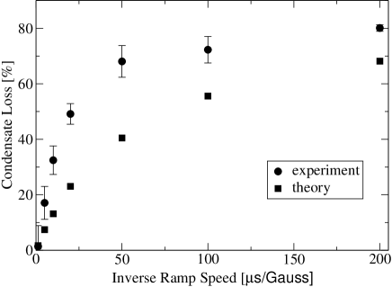
Figure 1: Loss of atoms from a ⁸⁵Rb condensate at the end of a linear magnetic field ramp across the 155 Gauss Feshbach resonance as a function of the inverse ramp speed. The circles with error bars are the experimental data from Ref. Cornish00 . The squares are determined from Eq. (9) using a cylindrical trap potential with the experimental trap frequencies.

We have employed the non-Markovian equation of the first-order cumulant approach to study other situations where significant loss of condensate atoms due to a dynamic perturbation is observed. The method has been successful in predicting the rate of atom loss in four-wave mixing experiments TKKB02 . We have also analysed TKTGKB03 the experiment pioneering the use of magnetic-field pulses for the association of molecules, where coherent atom-molecule oscillations have been observed Donley02 . In this context, the physical consequences of an extremely long-range nature of molecules created have been pointed out TKTGPSJKB03 and the process of adiabatic association of dimer molecules through Feshbach resonance crossings has been analysed in detail KGTKSAGETPSJ03 . The second-order approach has been used to determine the mean field energy associated with three-body collisions in Bose condensates TK02 .

There are other situations of experimental and theoretical interest where the mean-field dynamical description can be expected to fail due to the significance of pair correlations. In the context of optical lattices, the cumulant approach could be a useful tool in describing the dynamics of the superfluid bosonic gas in the vicinity of the quantum phase transition, where quantum depletion starts to grow. An area relatively unexplored experimentally is the dynamic manipulation of magnetically-tunable interactions, not necessarily in the close vicinity of a Feshbach resonance Abdullaev03 . The question of adiabaticity of the evolution with respect to particle loss from the condensate is an important one in this context. Finally, one can study situations where a Bose condensate is subjected to rapid variations of an external (e.g. trapping) potential. One of the interesting proposals in this field is a delta-kicked oscillator setup, employed in the studies of quantum chaos Gardiner00 .

From the viewpoint of the classical field methods, the cumulant approach also may offer an interesting perspective. The non-Markovian equation (9) can be viewed as a consistent way of including quantum corrections in the classical-field treatment. As such, it can be used to test the validity of replacing quantum field operators by complex-valued functions, which is the backbone of the latter approach Svistunov91 ; Damle96 ; Goral01 ; Davis01 ; Sinatra01 ; Goral02 ; Schmidt03 .

To conclude: in this paper we have reviewed a new method of tackling the dynamics of correlations in a Bose condensate, in terms of noncommutative cumulants. This framework delivers an accurate but computationally feasible approach to the beyond-mean-field evolution in a Bose-condensed gas. The method has been used to address several issues of current interest. Finally, we have pointed out several new applications and a possible link to the classical-field methods for partly condensed Bose gases.

We are particularly grateful to Eleanor Hodby, Simon Cornish and Carl Wieman for providing the experimental data in Fig. 1. We would also like to thank Simon Gardiner and Paul Julienne for many interesting discussions. This research has been supported by the European Community Marie Curie Fellowship under Contract no. HPMF-CT-2002-02000 (K.G.), a University Research Fellowship of the Royal Society (T.K.), Deutsche Forschungsgemeinschaft (T.G.). K.B. thanks the Royal Society and the Wolfson Foundation.

References

- (1) M.H. Anderson, J.R. Ensher, M.R. Matthews, C.E. Wieman, and E.A. Cornell, Science 269, 198 (1995).
- (2) M.R. Matthews, B.P. Anderson, P.C. Haljan, D.S. Hall, C.E.Wieman, and E.A. Cornell, Phys. Rev. Lett. 83, 2498 (1999).
- (3) K.W. Madison, F. Chevy, W. Wohlleben, and J. Dalibard, Phys. Rev. Lett. 84, 806 (2000).
- (4) S. Jochim, M. Bartenstein, A. Altmeyer, G. Hendl, S. Riedl, C. Chin, J. Hecker Denschlag, and R. Grimm, Science 302, 2101 (2003).
- (5) B. Goss Levi, Physics Today 56, no. 10, 18 (2003).
- (6) L.P. Pitaevskii, Zh. ksp. Teor. Fiz. 40, 646 (1961) [Sov. Phys. JETP 13, 451 (1961)].
- (7) E.P. Gross, Nuovo Cimento 20, 454 (1961).
- (8) F. Dalfovo, S. Giorgini, L.P. Pitaevskii, and S. Stringari, Rev. Mod. Phys. 71, 463 (1999).
- (9) B.V. Svistunov, J. Mosc. Phys. Soc. 1, 373 (1991).
- (10) K. Damle, S.N. Majumdar, and S. Sachdev, Phys. Rev. A 54, 5037 (1996).
- (11) K. Góral, M. Gajda, and K. Rza⸦żewski, Opt. Express 8, 92 (2001).
- (12) M.J. Davis, S.A. Morgan, and K. Burnett, Phys. Rev. Lett. 87, 160402 (2001).
- (13) A. Sinatra, C. Lobo, and Y. Castin, Phys. Rev. Lett. 87, 210404 (2001).
- (14) K. Góral, M. Gajda, and K. Rza⸦żewski, Phys. Rev. A 66, 051602 (2002).
- (15) H. Schmidt, K. Góral, F. Floegel, M. Gajda, and K. Rza⸦żewski, J. Opt. B: Quantum Semiclass. Opt. 5, S96 (2003).
- (16) M. Greiner, O. Mandel, T. Esslinger, T.W. Hänsch, and I. Bloch, Nature (London) 415, 39 (2002).
- (17) S. Inouye, M.R. Andrews, J. Stenger, H.-J. Miesner, D.M. Stamper-Kurn, and W. Ketterle, Nature (London) 392, 151 (1998).
- (18) E.A. Donley, N.R. Claussen, S.T. Thompson, and C.E. Wieman, Nature (London) 417, 529 (2002).
- (19) J. Herbig, T. Kraemer, M. Mark, T. Weber, C. Chin, H.-Ch. Nägerl, and R. Grimm, Science 301, 1510 (2003).
- (20) K. Xu, T. Mukaiyama, J.R. Abo-Shaeer, J.K. Chin, D. Miller, and W. Ketterle, Phys. Rev. Lett. 91, 210402 (2003).
- (21) S. Dürr, T. Volz, A. Marte, and G. Rempe, Phys. Rev. Lett. 92, 020406 (2004).
- (22) K. Góral, T. Köhler, S.A. Gardiner, E. Tiesinga, and P.S. Julienne, e-print arXive cond-mat/0312178.
- (23) T. Köhler and K. Burnett, Phys. Rev. A 65, 033601 (2002).
- (24) J. Fricke, Ann. Phys. (N.Y.) 252, 479 (1996).
- (25) S.L. Cornish, N.R. Claussen, J.L. Roberts, E.A. Cornell, and C.E. Wieman, Phys. Rev. Lett. 85, 1795 (2000).
- (26) We describe the state of the many-body system with the help of a statistical operator and the expectation value of an arbitrary operator in this state is given by . The evolution of such an expectation value is then determined by the Schrödinger equation .
- (27) T. Köhler, T. Gasenzer, and K. Burnett, Phys. Rev. A 67, 013601 (2003).
- (28) T. Köhler, K. Góral, and T. Gasenzer, e-print arXive cond-mat/0305060.
- (29) T. Köhler, T. Gasenzer, P.S. Julienne, and K. Burnett, Phys. Rev. Lett. 91, 230401 (2003).
- (30) T. Köhler, Phys. Rev. Lett. 89, 210404 (2002).
- (31) see, e.g., P.G. Kevrekidis, G. Theocharis, D.J. Frantzeskakis, and B.A. Malomed, Phys. Rev. Lett. 90, 230401 (2003).
- (32) S.A. Gardiner, D. Jaksch, R. Dum, J.I. Cirac, and P. Zoller, Phys. Rev. A 62, 023612 (2000).