Entanglement in Mesoscopic Structures: Role of Projection

Abstract

We present a theoretical analysis of the appearance of entanglement in non-interacting mesoscopic structures. Our setup involves two oppositely polarized sources injecting electrons of opposite spin into the two incoming leads. The mixing of these polarized streams in an ideal four-channel beam splitter produces two outgoing streams with particular tunable correlations. A Bell inequality test involving cross-correlated spin-currents in opposite leads signals the presence of spin-entanglement between particles propagating in different leads. We identify the role of fermionic statistics and projective measurement in the generation of these spin-entangled electrons.

Quantum entangled charged quasi-particles are perceived as a valuable resource for a future solid state based quantum information technology. Recently, specific designs for mesoscopic structures have been proposed which generate spatially separated streams of entangled particles ent_sc ; ent_qd ; chtchelkatchev_02 ; samuelsson_03 . In addition, Bell inequality type measurements have been conceived which test for the presence of these non-classical and non-local correlations chtchelkatchev_02 ; samuelsson_03 . Usually, entangled electron-pairs are generated through specific interactions (e.g., through the attractive interaction in a superconductor or the repulsive interaction in a quantum dot) and particular measures are taken to separate the constituents in space (e.g., involving beam splitters and appropriate filters). However, recently it has been predicted that non-local entanglement as signalled through a violation of Bell inequality tests can be observed in non-interacting systems as well beenakker_03 ; fazio_03 ; samuelsson_04 ; lebedev_03 . The important task then is to identify the origin of the entanglement; candidates are the fermionic statistics, the beam splitter, or the projection in the Bell measurement itself bosehome_02 ; samuelsson_04 .

Here, we report on our study of entanglement in a non-interacting system, where we make sure, that the particles encounter the Bell setup in a non-entangled state. Nevertheless, we find the Bell-inequality to be violated and conclude that the concomittant entanglement is produced in a wave function projection during the Bell measurement. We note that wave function projection as a resource of non-local entanglement is known for single-particle sources (Fock states) bosehome_02 , a scheme working for both bosons and fermions. What is different in Refs. beenakker_03, ; fazio_03, ; samuelsson_04, ; lebedev_03, and in the present work is that the sources are many-particle states in local thermal equilibrium. It is then essential that one deals with fermions; wave function projection cannot create entanglement out of a thermal source of bosons.

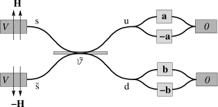
Figure 1: Mesoscopic normal-metal structure with a beam splitter generating two streams of electrons with tunable correlations in the two outgoing arms ‘u’ and ‘d’. The source (left) injects polarized (along the $z$-axis) electrons into the source leads ‘s’ and ‘$\bar{\mathrm{s}}$’. The beam splitter mixes the two incoming streams with a mixing angle $\vartheta$. The scattered (or outgoing) beams are analyzed in a Bell type coincidence measurement involving spin-currents projected onto the directions $\pm{\bf a}$ (in the ‘u’ lead) and $\pm{\bf b}$ (in the ‘d’ lead). The injection reservoirs are voltage ($V$) biased against the outgoing reservoirs. The Bell inequality test signals the presence of entanglement within the interval $|\vartheta-45^{\circ}|<12.235^{\circ}$. We relate this entanglement to the presence of spin-triplet correlations in the projected part of the scattered wavefunction describing electron-pairs distributed between the arms.

The generic setup for the production of spatially separated entangled degrees of freedom usually involves a source injecting the particles carrying the internal degree of freedom (the spin ent_sc ; ent_qd ; fazio_03 ; lebedev_03 or an orbital quantum number samuelsson_03 ; beenakker_03 ; samuelsson_04 ) and a beam splitter separating these particles in space, see Fig. 1. In addition, ‘filters’ may be used to inhibit the propagation of unwanted components into the spatially separated leads ent_sc ; ent_qd ; chtchelkatchev_02 ; samuelsson_03 , thus enforcing a pure flow of entangled particles in the outgoing leads. The successful generation of entanglement then is measured in a Bell inequality type setup BItest . A surprising new feature has been recently predicted with a Bell inequality test exhibiting violation in a non-interacting system beenakker_03 ; fazio_03 ; samuelsson_04 ; lebedev_03 ; the question arises as to what produces the entanglement manifested in the Bell inequality violation and it is this question which we wish to address in the present work. In order to do so, we describe theoretically an experiment where we make sure, that the particles are not entangled up to the point where the correlations are measured in the Bell inequality setup; nevertheless, we find them violated. We trace this violation back to an entanglement which has its origin in the confluence of various elements: i) the Fermi statistics provides a noiseless stream of incoming electrons, ii) the beam splitter mixes the indistinguishable particles at one point in space removing the information about their origin, iii) the splitter directs the mixed product state into the two leads thus organizing their spatial separation, iv) a coincidence measurement projects the mixed product state onto its (spin-)entangled component describing the electron pair split between the two leads, v) measuring the spin-entangled state in a Bell inequality test exhibits violation (the steps iv) and v) are united in our setup). Note, that the simple fermionic reservoir defining the source in Ref. lebedev_03, injects spin-entangled pairs from the beginning; hence an analysis of this system cannot provide a definitive answer on the minimal setup providing spatially separated entangled pairs since both the source and/or the projective Bell measurement could be responsible for the violation.

Below, we pursue the following strategy: We first define a particle source and investigate its characteristic via an analysis of the associated two-particle density matrix. We then define the corresponding pair wave function (thus reducing the many body problem to a two-particle problem) and determine its concurrence following the definition of Schliemann et al. schliemann_01 for indistinguishable particles (more generally, one could calculate the Slater rank of the wave function, cf. Ref. schliemann_01, ; here, we deal with a four-dimensional one-particle Hilbert space where the concurrence provides a simple and quantitative measure for the degree of entanglement). For our specially designed source we find a zero concurrence and hence our incoming beam is not entangled. We then go over to the scattering state behind the (tunable) beam splitter and reanalyze the state with the help of the two-particle density matrix. We determine the associated two-particle wave function and find its concurrence; comparing the results for the incoming and scattered wave function, we will see that the concurrence is unchanged, a simple consequence of the unitary action of the beam splitter. However, the mixer removes the information on the origin of the particles, thus preparing an entangled wave function component in the output channel. Third, we analyze the component of the wave function to which the Bell setup is sensitive and determine its degree of entanglement; depending on the mixing angle of the beam splitter, we find concurrencies between 0 (no entanglement) and unity (maximal entanglement). Finally, we determine the violation of the Bell inequality as measured through time-resolved spin-current cross-correlators and find agreement between the degree of violation and the degree of entanglement of the projected state as expressed through the concurrence.

Our source draws particles from two spin-polarized reservoirs with opposite polarization directed along the $z$-axis. The polarized electrons are injected into source leads ‘s’ and ‘$\bar{\rm s}$’ and are subsequently mixed in a tunable four-channel beam splitter, see Fig. 1. The outgoing channels are denoted by ‘u’ (for the upper lead) and ‘d’ (the ‘down’ lead). The spin-correlations in the scattering channels ‘u’ and ‘d’ are then analyzed in a Bell inequality test. The polarized reservoirs are voltage biased with $eV=\mu_{\rm\scriptscriptstyle B}H/2$ equal to the magnetic energy in the polarizing field $H$; the incoming electron streams then are fully polarized (the magnetic field is confined to the reservoirs).

The spin-correlations between electrons in leads ‘x’ and ‘y’ are conveniently analyzed with the help of the two-particle density matrix (or pair correlation function)

$$g_{\vec{\sigma}}^{\mathrm{xy}}(x,y)=\mathrm{Tr}\bigl{(}\hat{\rho}\hat{\Psi}_{\mathrm{x}\sigma_{1}}^{\dagger}(x)\hat{\Psi}_{\mathrm{y}\sigma_{2}}^{\dagger}(y)\hat{\Psi}_{\mathrm{y}\sigma_{3}}(y)\hat{\Psi}_{\mathrm{x}\sigma_{4}}(x)\bigr{)}$$ (1)

with trace over states of the Fermi sea. Here, $\hat{\Psi}_{\mathrm{x}\sigma}$ are field operators describing electrons with spin $\sigma$ in lead ‘x’ and $\hat{\rho}$ is the density operator. The pair correlation function (1) is conveniently expressed through the one-particle correlators $G_{\sigma\bar{\sigma}}^{\mathrm{xy}}(x,y)\equiv\langle\hat{\Psi}_{\mathrm{x}\sigma}^{\dagger}(x)\hat{\Psi}_{\mathrm{y}\bar{\sigma}}(y)\rangle$,

$$g_{\vec{\sigma}}^{\mathrm{xy}}(x,y)\!=\!G_{\sigma_{1}\!\sigma_{4}}^{\mathrm{xx}}\!(0)G_{\sigma_{2}\!\sigma_{3}}^{\mathrm{yy}}\!(0)-G_{\sigma_{1}\!\sigma_{3}}^{\mathrm{xy}}\!(x\!-\!y)G_{\sigma_{2}\!\sigma_{4}}^{\mathrm{yx}}\!(y\!-\!x).$$ (2)

The one-particle correlators can be written in terms of a product of orbital- and spin parts, $G_{\sigma\bar{\sigma}}^{\mathrm{xy}}(x,y)=G^{\mathrm{xy}}(x,y)\chi^{\mathrm{xy}}(\sigma,\bar{\sigma})$, and split into equilibrium and excess terms,

$$G_{\sigma\bar{\sigma}}^{\mathrm{xy}}(x,y)=G_{\mathrm{eq}}(x,y)\chi_{\mathrm{eq}}^{\mathrm{xy}}(\sigma,\bar{\sigma})+G_{\mathrm{ex}}(x,y)\chi_{\mathrm{ex}}^{\mathrm{xy}}(\sigma,\bar{\sigma}),$$ (3)

with $G_{\mathrm{ex}}(x,y)$ vanishing at zero voltage $V$ and zero polarization field $H$.

In order to find the two-particle density matrix in the source leads ‘s’, ‘$\bar{\mathrm{s}}$’ we make use of the scattering states

$$\hat{\Psi}_{\mathrm{s}}\!=\!\sum\limits_{k\sigma}e^{ikx}\hat{a}_{k\sigma}+e^{-ikx}(\cos\vartheta e^{-i\varphi}\hat{c}_{k\sigma}+\sin\vartheta e^{i\psi}\hat{d}_{k\sigma}),$$

$$\hat{\Psi}_{\bar{\mathrm{s}}}\!=\!\sum\limits_{k\sigma}e^{ikx}\hat{b}_{k\sigma}+e^{-ikx}(\cos\vartheta e^{i\varphi}\hat{d}_{k\sigma}-\sin\vartheta e^{-i\psi}\hat{c}_{k\sigma}),$$

where $\hat{a}_{k\sigma}$, $\hat{b}_{k\sigma}$ denote the annihilation operators for electrons in the source reservoirs $\mathrm{s}$ and $\bar{\mathrm{s}}$ with momentum $k$ and spin $\sigma\in\uparrow,\downarrow$ polarized along the $z$-axis and time evolution $\propto\exp(-i\epsilon_{k}t/\hbar)$, $\epsilon_{k}=\hbar^{2}k^{2}/2m$; the operators $\hat{c}_{k\sigma}$ and $\hat{d}_{k\sigma}$ annihilate electrons in the reservoirs attached to the outgoing leads ‘u’ and ‘d’, respectively. Also, we make use here of the standard parametrization of a reflectionless four-beam splitter,

$$\left(\begin{array}[]{c}\mathrm{u}\\ \mathrm{d}\end{array}\right)=\left(\begin{array}[]{cc}e^{i\varphi}\cos\vartheta&-e^{i\psi}\sin\vartheta\\ e^{-i\psi}\sin\vartheta&e^{-i\varphi}\cos\vartheta\end{array}\right)\left(\begin{array}[]{c}\mathrm{s}\\ \bar{\mathrm{s}}\end{array}\right),$$ (4)

with the angles $\vartheta\in(0,\pi/2)$, $\varphi,\psi\in(0,2\pi)$; without loss of generality we will assume $\varphi=\psi=0$ in what follows. The orbital part of the one-particle correlator $G^{\mathrm{xy}}(x-y)\equiv G(x-y)$ takes the form

$$G_{\mathrm{eq}}(x)=\frac{\sin k_{\rm\scriptscriptstyle F}}{\pi x},$$ (5)

$$G_{\mathrm{ex}}(x)=e^{-i(k_{\rm\scriptscriptstyle F}+k_{V})x}\,\frac{\sin k_{V}x}{\pi x},$$ (6)

with $k_{V}=k_{\rm\scriptscriptstyle F}(eV/\epsilon_{\rm\scriptscriptstyle F})$ and $\epsilon_{\rm\scriptscriptstyle F}$ ($k_{\rm\scriptscriptstyle F}$) the Fermi energy (wave vector) in the unbiased system. The spin factors for the equilibrium and excess parts read,

$$\chi_{\mathrm{eq}}^{\mathrm{xx}}(\sigma,\bar{\sigma})=\langle\sigma|\bar{\sigma}\rangle,$$ (7)

$$\chi_{\mathrm{ex}}^{\mathrm{ss}}(\sigma,\bar{\sigma})\!=\!\langle\sigma|\!\uparrow\rangle\langle\uparrow\!|\bar{\sigma}\rangle,\quad\chi_{\mathrm{ex}}^{\mathrm{\bar{s}\,\bar{s}}}(\sigma,\bar{\sigma})\!=\!\langle\sigma|\!\downarrow\rangle\langle\downarrow\!|\bar{\sigma}\rangle,$$

the latter describing the injection of polarized electrons into the leads ‘s’ and ‘$\bar{\mathrm{s}}$’. Finally, the cross correlation function between the source leads vanishes, $G_{\sigma\bar{\sigma}}^{\mathrm{\,s\bar{s}}}(x-y)=0$, and the final result for the excess part of the pair correlation function between source leads reads

$$\bigl{[}g^{\mathrm{\,s\bar{s}}}_{\vec{\sigma}}(x,y)\bigr{]}_{\mathrm{ex}}=|G_{\mathrm{ex}}(0)|^{2}\,\langle\sigma_{1}|\!\uparrow\rangle\langle\uparrow\!|\sigma_{4}\rangle\langle\sigma_{2}|\!\downarrow\rangle\langle\downarrow\!|\sigma_{3}\rangle.$$ (8)

This result then describes the injection of two uncorrelated streams of polarized electrons into the leads ‘s’ and ‘$\bar{\mathrm{s}}$’. Furthermore, statistical analysis lesoviklevitov tells that the Fermi statistics enforces injection into each lead of a regular stream of particles separated by the single-particle correlation time $\tau_{V}=\hbar/eV$. The full many body description then is conveniently reduced to a two-particle problem where the two reservoirs inject a sequence of electron pairs residing in the wave function $\Psi_{\mathrm{in}}^{\scriptscriptstyle 12}=\bigl{[}\phi_{\mathrm{s}\uparrow}^{\scriptscriptstyle 1}\phi_{\bar{\mathrm{s}}\downarrow}^{\scriptscriptstyle 2}-\phi_{\bar{\mathrm{s}}\downarrow}^{\scriptscriptstyle 1}\phi_{\mathrm{s}\uparrow}^{\scriptscriptstyle 2}\bigr{]}/\sqrt{2}$ with $\phi_{\mathrm{s}\uparrow}$ ($\phi_{\bar{\mathrm{s}}\downarrow}$) the single-particle wave functions associated with electrons in the upper (lower) source lead. This wave function is a simple Slater determinant and hence non-entangled according to schliemann_01 .

Next, we extend the above analysis to the outgoing leads ‘u’ and ‘d’. The scattering states in the outgoing leads take the form

$$\hat{\Psi}_{\mathrm{u}}=\!\sum\limits_{k\sigma}e^{-ikx}\hat{c}_{k\sigma}\!+e^{ikx}(\cos\vartheta\,\hat{a}_{k\sigma}-\sin\vartheta\,\hat{b}_{k\sigma}),$$

$$\hat{\Psi}_{\mathrm{d}}=\!\sum\limits_{k\sigma}e^{-ikx}\hat{d}_{k\sigma}\!+e^{ikx}(\cos\vartheta\,\hat{b}_{k\sigma}+\sin\vartheta\,\hat{a}_{k\sigma}).$$

The excess particles injected by the source leads now are mixed in the beam-splitter and thus non-vanishing cross correlations are expected to show up in the leads ‘u’ and ‘d’. The one-particle correlation function assumes the form (3) with the orbital correlators (5) and (6) and spin correlators

$$\chi_{\mathrm{eq}}^{\mathrm{xx}}(\sigma,\bar{\sigma})=\langle\sigma|\bar{\sigma}\rangle,\qquad\mathrm{x}\in{\text{`u'}},{\text{`d'}},$$ (9)

$$\chi_{\mathrm{ex}}^{\mathrm{uu}}(\sigma,\bar{\sigma})=\cos^{2}\vartheta\langle\sigma|\!\uparrow\rangle\langle\uparrow\!|\bar{\sigma}\rangle+\sin^{2}\vartheta\langle\sigma|\!\downarrow\rangle\langle\downarrow\!|\bar{\sigma}\rangle,$$

$$\chi_{\mathrm{ex}}^{\mathrm{dd}}(\sigma,\bar{\sigma})=\sin^{2}\vartheta\langle\sigma|\!\uparrow\rangle\langle\uparrow\!|\bar{\sigma}\rangle+\cos^{2}\vartheta\langle\sigma|\!\downarrow\rangle\langle\downarrow\!|\bar{\sigma}\rangle,$$

$$\chi_{\mathrm{ex}}^{\mathrm{ud}}(\sigma,\bar{\sigma})=\chi_{\mathrm{ex}}^{\mathrm{du}}(\sigma,\bar{\sigma})$$

$$\qquad\qquad\,\,=\cos\vartheta\sin\vartheta\bigl{[}\langle\sigma|\!\uparrow\rangle\langle\uparrow\!|\bar{\sigma}\rangle-\langle\sigma|\!\downarrow\rangle\langle\downarrow\!|\bar{\sigma}\rangle\bigr{]}.$$

Evaluating the excess part of the two-particle cross-correlations between the leads ‘u’ and ‘d’ at the symmetric position $x=y$ we find

$$\bigl{[}g^{\mathrm{ud}}_{\vec{\sigma}}(x,x)\bigr{]}_{\mathrm{ex}}=|G_{\mathrm{ex}}(0)|^{2}$$ (10)

$$\qquad\,\,\,\bigl{[}\cos^{4}\vartheta\langle\sigma_{1}|\!\uparrow\rangle\langle\uparrow\!|\sigma_{4}\rangle\langle\sigma_{2}|\!\downarrow\rangle\langle\downarrow\!|\sigma_{3}\rangle$$

$$\qquad+\sin^{4}\vartheta\langle\sigma_{1}|\!\downarrow\rangle\langle\downarrow\!|\sigma_{4}\rangle\langle\sigma_{2}|\!\uparrow\rangle\langle\uparrow\!|\sigma_{3}\rangle$$

$$\qquad+\cos^{2}\vartheta\sin^{2}\vartheta\langle\sigma_{1}|\!\uparrow\rangle\langle\uparrow\!|\sigma_{3}\rangle\langle\sigma_{2}|\!\downarrow\rangle\langle\downarrow\!|\sigma_{4}\rangle$$

$$\qquad+\cos^{2}\vartheta\sin^{2}\vartheta\langle\sigma_{1}|\!\downarrow\rangle\langle\downarrow\!|\sigma_{3}\rangle\langle\sigma_{2}|\!\uparrow\rangle\langle\uparrow\!|\sigma_{4}\rangle\bigr{]}.$$

Hence, a symmetric splitter ($\vartheta=\pi/4$) produces the spin correlations of a triplet state $[|\chi_{\mathrm{tr}}^{\mathrm{ud}}\rangle=|\!\uparrow\rangle_{\mathrm{u}}|\!\downarrow\rangle_{\mathrm{d}}+$ $|\!\downarrow\rangle_{\mathrm{u}}|\!\uparrow\rangle_{\mathrm{d}}]/\sqrt{2}$ involving two electrons separated in different leads ‘u’ and ‘d’ but at equivalent locations $x=y$. The general case with arbitrary mixing angle $\vartheta$ results in a density matrix describing a pure state involving the superposition $|\chi_{\mathrm{tr}}^{\mathrm{ud}}\rangle+\cos 2\vartheta|\chi_{\mathrm{sg}}^{\mathrm{ud}}\rangle$ of the above triplet state and the singlet state $[|\chi_{\mathrm{sg}}^{\mathrm{ud}}\rangle=|\!\uparrow\rangle_{\mathrm{u}}|\!\downarrow\rangle_{\mathrm{d}}-|\!\downarrow\rangle_{\mathrm{u}}|\!\uparrow\rangle_{\mathrm{d}}]/\sqrt{2}$. The analoguous calculation for the two-particle density matrix describing electrons in the same outgoing lead ‘x’ equal ’u’ or ’d’ points to the presence of singlet correlations,

$$\bigl{[}g^{\mathrm{xx}}_{\vec{\sigma}}(x,y)\bigr{]}_{\mathrm{ex}}=|G_{\mathrm{ex}}(0)|^{2}\langle\sigma_{1}|\sigma_{4}\rangle\langle\sigma_{2}|\sigma_{3}\rangle$$ (11)

$$\qquad\qquad-\,|G_{\mathrm{ex}}(x-y)|^{2}\langle\sigma_{1}|\sigma_{3}\rangle\langle\sigma_{2}|\sigma_{4}\rangle.$$

Again, the above results can be used to reduce the problem from its many-body form to a two-particle problem. Given the incoming Slater determinant $\Psi_{\mathrm{in}}^{\scriptscriptstyle 12}$ we obtain the scattered state $\Psi_{\mathrm{out}}^{\scriptscriptstyle 12}$ through the transformation $\phi_{\mathrm{s}\uparrow}\rightarrow\cos\vartheta\,\phi_{\mathrm{u}\uparrow}+\sin\vartheta\,\phi_{\mathrm{d}\uparrow}$ describing scattered spin-$\uparrow$ electrons originating from the source lead ‘s’ and $\phi_{\bar{\mathrm{s}}\downarrow}\rightarrow-\sin\vartheta\,\phi_{\mathrm{u}\downarrow}+\cos\vartheta\,\phi_{\mathrm{d}\downarrow}$ for excess spin-$\downarrow$ electrons from ‘$\bar{\mathrm{s}}$’ (the wave functions $\phi_{\mathrm{x}\sigma}=\phi_{\mathrm{x}}\chi_{\sigma}$ describe electrons with orbital (spin) wave function $\phi_{\mathrm{x}}$ ($\chi_{\sigma}$) propagating in lead ‘x’). The resulting scattering wave function has the form

$$\Psi_{\mathrm{out}}^{\scriptscriptstyle 12}=\sin\vartheta\cos\vartheta\bigl{[}\phi_{\mathrm{u}}^{\scriptscriptstyle 1}\phi_{\mathrm{u}}^{\scriptscriptstyle 2}\chi_{\mathrm{sg}}^{\scriptscriptstyle 12}-\phi_{\mathrm{d}}^{\scriptscriptstyle 1}\phi_{\mathrm{d}}^{\scriptscriptstyle 2}\chi_{\mathrm{sg}}^{\scriptscriptstyle 12}\bigr{]}$$

$$\qquad\>\>+\Phi_{\mathrm{ud}}^{\scriptscriptstyle 12}\chi_{\mathrm{tr}}^{\scriptscriptstyle 12}+\cos 2\vartheta\,\bar{\Phi}_{\mathrm{ud}}^{\scriptscriptstyle 12}\chi_{\mathrm{sg}}^{\scriptscriptstyle 12},$$ (12)

where the first two terms describe the propagation of a spin-singlet pair with the wave function $\chi_{\mathrm{sg}}^{\scriptscriptstyle 12}=(\chi_{\uparrow}^{\scriptscriptstyle 1}\chi_{\downarrow}^{\scriptscriptstyle 2}-\chi_{\downarrow}^{\scriptscriptstyle 1}\chi_{\uparrow}^{\scriptscriptstyle 2})/\sqrt{2}$ in the upper and lower lead. The last two terms describe the component where the electron pair is split between the ‘u’ and ‘d’ leads; it is a superposition of singlet- and triplet states ($\chi_{\mathrm{tr}}^{\scriptscriptstyle 12}=(\chi_{\uparrow}^{\scriptscriptstyle 1}\chi_{\downarrow}^{\scriptscriptstyle 2}+\chi_{\downarrow}^{\scriptscriptstyle 1}\chi_{\uparrow}^{\scriptscriptstyle 2})/\sqrt{2}$) with corresponding symmetrized and anti-symmetrized orbital wave functions $\bar{\Phi}_{\mathrm{ud}}^{\scriptscriptstyle 12}=(\phi_{\mathrm{u}}^{\scriptscriptstyle 1}\phi_{\mathrm{d}}^{\scriptscriptstyle 2}+\phi_{\mathrm{d}}^{\scriptscriptstyle 1}\phi_{\mathrm{u}}^{\scriptscriptstyle 2})/2$ and $\Phi_{\mathrm{ud}}^{\scriptscriptstyle 12}=(\phi_{\mathrm{u}}^{\scriptscriptstyle 1}\phi_{\mathrm{d}}^{\scriptscriptstyle 2}-\phi_{\mathrm{d}}^{\scriptscriptstyle 1}\phi_{\mathrm{u}}^{\scriptscriptstyle 2})/2$. The entanglement present in these wave functions is easily determined using the formalism developed by Schliemann et al. schliemann_01 : The wave function associated with a pair of electrons can be written in terms of a single-electron basis $\{\phi_{i}\}$, $\Psi^{\scriptscriptstyle 12}=\sum_{ij}\phi_{i}^{\scriptscriptstyle 1}w_{ij}\phi_{j}^{\scriptscriptstyle 2}$ where the anti-symmetric matrix $w_{ij}=-w_{ji}$ guarantees for the proper symmetrization. The analysis simplifies drastically for the case where the one-particle Hilbert space is four-dimensional; then the concurrence ${\cal C}(\Psi)=8\sqrt{\det w(\Psi)}$ gives a quantitative measure for the entanglement present in the wave function $\Psi$, ${\cal C}(\Psi)=0$ for a non-entangled state and ${\cal C}(\Psi)=1$ for a fully entangled wave function. For our setup the one-particle basis is defined as $\{\phi_{\mathrm{u}\uparrow},\phi_{\mathrm{u}\downarrow},\phi_{\mathrm{d}\uparrow},\phi_{\mathrm{d}\downarrow}\}$ and the matrix $w(\Psi_{\mathrm{out}})$ describing the scattered state (12) assumes the form

$$w^{\mathrm{out}}_{ij}=\!\frac{1}{\sqrt{2}}\!\!\left[\!\begin{array}[]{cccc}0&-{\sin 2\vartheta}/2&0&\cos^{2}\vartheta\\ \sin 2\vartheta/2&0&\sin^{2}\vartheta&0\\ 0&-\sin^{2}\vartheta&0&\sin 2\vartheta/2\\ -\cos^{2}\vartheta&0&-\sin 2\vartheta/2&0\end{array}\!\right]\!.$$ (17)

The concurrence of the scattering state (12) vanishes, hence $\Psi^{\mathrm{out}}$ is non-entangled and takes the form of an elementary Slater determinant. Next, let us analyze the concurrence of that part of the scattering wave function to which our coincidence measurement in leads ‘u’ and ‘d’ is sensitive. The component describing the two particles split between the leads reads $\Psi_{\mathrm{ud}}^{\scriptscriptstyle 12}=\Phi_{\mathrm{ud}}^{\scriptscriptstyle 12}\chi_{\mathrm{tr}}^{\scriptscriptstyle 12}+\cos 2\vartheta\,\bar{\Phi}_{\mathrm{ud}}^{\scriptscriptstyle 12}\chi_{\mathrm{sg}}^{\scriptscriptstyle 12}$, cf. (12). This projected state is described by the matrix

$$w^{\mathrm{ud}}_{ij}=\frac{1}{\sqrt{2}}\left[\!\begin{array}[]{cccc}0&0&0&\cos^{2}\vartheta\\ 0&0&\sin^{2}\vartheta&0\\ 0&-\sin^{2}\vartheta&0&0\\ -\cos^{2}\vartheta&0&0&0\end{array}\!\right],$$ (22)

from which one easily derives the concurrence ${\cal C}(\Psi_{\mathrm{ud}}^{\scriptscriptstyle 12})=\sin^{2}2\vartheta$; we conclude that the component $\Psi_{\mathrm{ud}}^{\scriptscriptstyle 12}$ detected in a coincidence measurement is entangled. Furthermore, the concurrence is equal to unity for the symmetric splitter $\phi=\pi/4$ where we deal with a maximally entangled triplet state (note the loss of information about which electron (from ‘s’ or ‘$\bar{\mathrm{s}}$’) enters the lead ‘u’ or ‘d’). We conclude that a Bell inequality test sensitive to the split part of the wave function will exhibit violation. We attribute this violation to the combined action of i) the splitter where the information on the identity of the particles is destroyed and the entangled component $\Psi_{\mathrm{ud}}^{\scriptscriptstyle 12}$ is ‘prepared’ and ii) the wave function projection inherent in the coincidence measurement and ‘realizing’ the entanglement.

The Bell type setup BItest in Fig. 1 measures the correlations in the spin-entangled scattered wave function $\Psi_{\mathrm{out}}^{\scriptscriptstyle 12}$. It involves the finite-time current cross-correlators $C_{{\bf a},{\bf b}}(x,y;\tau)\equiv\langle\langle\hat{I}_{\bf a}(x,\tau)\hat{I}_{\bf b}(y,0)\rangle\rangle$ between the spin-currents $\hat{I}_{\bf a}(x,\tau)$ projected onto directions ${\bf a}$ (in lead ‘u’) and partners $\hat{I}_{\bf b}(y,0)$ (in lead ‘d’) projected onto ${\bf b}$. These correlators enter the Bell inequality ($\bar{\bf a}$ and $\bar{\bf b}$ denote a second set of directions)

$$|E({\bf a},{\bf b})-E({\bf a},\bar{\bf b})+E(\bar{\bf a},{\bf b})+E(\bar{\bf a},\bar{\bf b})|\leq 2$$ (23)

via the current difference correlators

$$E({\bf a},{\bf b})=\frac{\langle[\hat{I}_{\bf a}(\tau)-\hat{I}_{\bf-a}(\tau)][\hat{I}_{\bf b}(0)-\hat{I}_{\bf-b}(0)]\rangle}{\langle[\hat{I}_{\bf a}(\tau)+\hat{I}_{\bf-a}(\tau)][\hat{I}_{\bf b}(0)+\hat{I}_{\bf-b}(0)]\rangle}.$$ (24)

The cross-measurement in different leads implies that the setup is sensitive only to the spin-entangled split-pair part $\Psi_{\mathrm{ud}}^{\scriptscriptstyle 12}$ of the scattering wave function and hence the Bell inequality can be violated. Making use of the field operators $\hat{\Psi}_{\mathrm{u}}$ and $\hat{\Psi}_{\mathrm{d}}$ describing the scattering states in the outgoing leads, we determine the irreducible current cross correlator and factorize into orbital and spin parts, $C_{{\bf a},{\bf b}}(x,y;\tau)=C_{x,y}(\tau)F_{{\bf a},{\bf b}}$, with $F_{{\bf a},{\bf b}}$ accounting for the spin projections. Using standard scattering theory of noise noise , one obtains the orbital cross-correlator (only the excess part gives a finite contribution)

$$C_{x,y}(\tau)=-\frac{e^{2}\sin^{2}\!2\vartheta}{h^{2}}\sin^{2}\frac{eV(\tau\!-\!\tau_{-})}{\hbar}\,\alpha(\tau\!-\!\tau_{-},\theta),$$ (25)

with $\alpha(\tau,\theta)=\pi^{2}\theta^{2}/\sinh^{2}[\pi\theta\tau/\hbar]$, $\tau^{\pm}=(x\pm y)/v_{\rm\scriptscriptstyle F}$, $\theta$ the temperature of the electronic reservoirs, and $v_{\rm\scriptscriptstyle F}$ the Fermi velocity. In order to arrive at the result (25) we have dropped terms small in the parameter $|\epsilon^{\prime}-\epsilon|/\epsilon_{\rm\scriptscriptstyle F}$ noise . The spin projection $F_{{\bf a},{\bf b}}$ assumes the form

$$F_{{\bf a},{\bf b}}=\langle{\bf a}|\!\uparrow\rangle\langle\uparrow\!|{\bf b}\rangle\langle{\bf b}|\!\uparrow\rangle\langle\uparrow\!|{\bf a}\rangle+\langle{\bf a}|\!\downarrow\rangle\langle\downarrow\!|{\bf b}\rangle\langle{\bf b}|\!\downarrow\rangle\langle\downarrow\!|{\bf a}\rangle$$

$$\qquad\>-\,\langle{\bf a}|\!\uparrow\rangle\langle\uparrow\!|{\bf b}\rangle\langle{\bf b}|\!\downarrow\rangle\langle\downarrow\!|{\bf a}\rangle-\langle{\bf a}|\!\downarrow\rangle\langle\downarrow\!|{\bf b}\rangle\langle{\bf b}|\!\uparrow\rangle\langle\uparrow\!|{\bf a}\rangle.$$

We express this result in terms of the angles $\theta_{\bf a}$ and $\varphi_{\bf a}$ describing the direction of magnetization in the ‘u’ lead filters and $\theta_{\bf b}$, $\varphi_{\bf b}$ referring to the filters in the ‘d’ lead and find that $F_{{\bf a},{\bf b}}=F_{-{\bf a},-{\bf b}}=F^{+}_{{\bf a},{\bf b}}$, $F_{-{\bf a},{\bf b}}=F_{{\bf a},-{\bf b}}=F^{-}_{{\bf a},{\bf b}}$ and

$$F_{{\bf a},{\bf b}}^{\pm}\!=\!(1\!\pm\cos\theta_{\bf a}\cos\theta_{\bf b}\!\mp\!\cos\varphi_{{\bf a}{\bf b}}\sin\theta_{\bf a}\sin\theta_{\bf b})/2,$$

with $\varphi_{{\bf a}{\bf b}}=\varphi_{\bf a}-\varphi_{\bf b}$. The correlator $E({\bf a},{\bf b})$ takes the form

$$E({\bf a},{\bf b})=\frac{2C_{x,y}(\tau)\bigl{[}F_{{\bf a},{\bf b}}^{+}-F_{{\bf a},{\bf b}}^{-}\bigr{]}+\Lambda_{-}}{2C_{x,y}(\tau)\bigl{[}F_{{\bf a},{\bf b}}^{+}+F_{{\bf a},{\bf b}}^{-}\bigr{]}+\Lambda_{+}},$$

with $\Lambda_{\pm}=[\langle\hat{I}_{{\bf a}}\rangle\pm\langle\hat{I}_{{\bf-a}}\rangle][\langle\hat{I}_{{\bf b}}\rangle\pm\langle\hat{I}_{{\bf-b}}\rangle]$. Evaluating the projected current averages one obtains $\Lambda_{-}=-e^{2}\,(2eV/h)^{2}\cos\theta_{\bf a}\cos\theta_{\bf b}\cos^{2}2\vartheta$ and $\Lambda_{+}=e^{2}(2eV/h)^{2}$. The triplet state is rotationally invariant within the plane $\theta_{\bf a}=\theta_{\bf b}=\pi/2$ and choosing filters within this equatorial plane the Bell inequality takes the form

$$\Bigg{|}\frac{C_{x,y}(\tau)[\cos\varphi_{{\bf a}{\bf b}}\!-\cos\varphi_{{\bf a}\bar{\bf b}}\!+\cos\varphi_{\bar{\bf a}{\bf b}}\!+\cos\varphi_{\bar{\bf a}\bar{\bf b}}\bigr{]}}{2C_{x,y}(\tau)+\Lambda_{+}}\Bigg{|}\!\leq 1.$$

Its maximum violation is obtained for the set of angles $\varphi_{\bf a}=0$, $\varphi_{\bf b}=\pi/4$, $\varphi_{\bar{\bf a}}=\pi/2$, $\varphi_{\bar{\bf b}}=3\pi/4$,

$$E_{\rm\scriptscriptstyle BI}\equiv\left|\frac{2C_{x,y}(\tau)}{2C_{x,y}(\tau)+\Lambda_{+}}\right|\leq\frac{1}{\sqrt{2}}.$$ (26)

Evaluating the above expression in the limit of low temperatures $\theta<eV$ and at the symmetric position $x=y$, we arrive at the simple form

$$\frac{\sin^{2}2\vartheta\,\sin^{2}(eV\tau/\hbar\bigr{)}}{2(eV\tau/\hbar)^{2}-\sin^{2}2\vartheta\sin^{2}(eV\tau/\hbar)}\leq\frac{1}{\sqrt{2}}.$$ (27)

We observe that the violation of the Bell inequality is restricted to short times $\tau<\tau_{\rm\scriptscriptstyle BI}=\tau_{V}\equiv\hbar/eV$ (lebedev_03 ; the relevance of a coincidence measurement involving the short time $\tau_{V}$ was noticed in Refs. beenakker_03 ; samuelsson_03 ). Furthermore, the violation strongly depends on the mixing angle $\vartheta$ of the beam splitter, with a maximal violation realized for a symmetric splitter $\vartheta=\pi/4$ generating a pure triplet state across the two arms. The Bell inequality cannot be violated for asymmetric splitters with $|\vartheta-\pi/4|>0.2135$ (corresponding to an angular width $|\vartheta-45^{\circ}|>12.235^{\circ}$): evaluating the BI (27) at zero time difference (i.e., in a coincidence measurement) we find the condition

$$\frac{\sin^{2}2\vartheta}{2-\sin^{2}2\vartheta}\leq\frac{1}{\sqrt{2}},$$ (28)

from which one derives the critical angle $\vartheta_{c}=[{\rm arcsin}(2/(\sqrt{2}+1))^{1/2}]/2=0.572$ (or $\vartheta_{c}=32.765^{\circ}$). The appearance of a critical angle naturally follows from the fact that the measured wave function component $\Psi_{\mathrm{ud}}^{\scriptscriptstyle 12}$ assumes the form of a simple Slater determinant in the limits $\vartheta=0,\pi/2$ and hence is not entangled. Note that the product of average currents $\Lambda_{+}$ is the largest term in the denominator of (26) and hence always relevant.

In conclusion, we have described a mesoscopic setup with a source injecting non-entangled electron pairs into two source leads ‘s’ and ‘$\bar{\mathrm{s}}$’. Subsequent mixing of these particle streams in a four-channel beam splitter does not generate entanglement between the particles in the two output leads ‘u’ and ‘d’. However, proper mixing of the incoming beams in the splitter removes the information on the path of the incoming particles and generates a wave function component describing electrons split between the leads ‘u’ and ‘d’ which is entangled. It is this component which manifests itself in the coincidence measurement of a Bell inequality test and proper violation is observed at short times. This analysis answers the question regarding the origin of entanglement observed in the Bell inequality test applied to the present non-interacting system. A modified setup where the particles propagate downstream after a coincidence measurement lends itself as a source for spin-entangled particles, cf. Ref. bosehome_02, .

It is interesting to analyze the setup described in Ref. lebedev_03, in the light of the findings reported here. The setup in lebedev_03 involves a simple normal reservoir injecting pairs of electrons into a source lead which are subsequently separated in space by a beam splitter. The injected pairs reside in a spin-singlet state involving the identical orbital wave function, $\Psi_{\mathrm{in}}^{\scriptscriptstyle 12}=\phi_{\mathrm{s}}^{\scriptscriptstyle 1}\phi_{\mathrm{s}}^{\scriptscriptstyle 2}\chi_{\mathrm{sg}}^{\scriptscriptstyle 12}$; the entanglement observed in a Bell inequality test then has been attributed to the entanglement associated with this spin-singlet state. One may criticise, that this incoming singlet, being a simple Slater determinant, is not entangled according to the definition given by Schliemann et al. schliemann_01 . However, after the beam splitter the orbital wave function $\phi_{\mathrm{s}}$ is delocalized between the two leads, $\phi_{\mathrm{s}}\rightarrow\Phi=t_{\mathrm{su}}\phi_{\mathrm{u}}+t_{\mathrm{sd}}\phi_{\mathrm{d}}$, with $t_{\mathrm{su}}$ and $t_{\mathrm{sd}}$ the corresponding scattering amplitudes. While the scattered state remains a Slater determinant $\Psi_{\mathrm{out}}^{\scriptscriptstyle 12}=\Phi^{\scriptscriptstyle 1}\Phi^{\scriptscriptstyle 2}\chi_{\mathrm{sg}}^{\scriptscriptstyle 12}$, the singlet correlations now can be observed in a coincidence measurement testing the cross-correlations between the leads ‘u’ and ‘d’. Hence the spin-entanglement is produced by the reservoir, but its observation requires proper projection. It is then difficult to trace a unique origin for the entanglement manifested in the violation of a Bell inequality test. The appropriate setup to address this question should involve a reservoir injecting particles with opposite spin residing in a Slater determinant of the form $\Psi_{\mathrm{in}}^{\scriptscriptstyle 12}=[\phi_{\mathrm{s}\uparrow}^{\scriptscriptstyle 1}\bar{\phi}_{\mathrm{s}\downarrow}^{\scriptscriptstyle 2}-\bar{\phi}_{\mathrm{s}\downarrow}^{\scriptscriptstyle 1}\phi_{\mathrm{s}\uparrow}^{\scriptscriptstyle 2}]/\sqrt{2}$ which is not entangled in the spin variable. Such an analysis has been presented here with the result, that the orbital projection in the coincidence measurement is sufficient to produce a spin-entangled state.

We acknowledge discussions with Atac Imamoglu and financial support from the Swiss National Foundation (SCOPES and CTS-ETHZ), the Landau Scholarship of the FZ Jülich, the Russian Science Support Foundation, the Russian Ministry of Science, and the program ‘Quantum Macrophysics’ of the RAS.

References

• (1) G. Lesovik, Th. Martin, and G. Blatter, Eur. Phys. J. B 24, 287 (2001); P. Recher, E.V. Sukhorukov, and D. Loss, Phys. Rev. B 63, 165314 (2001); C. Bena et al., Phys. Rev. Lett. 89, 037901 (2002).
• (2) G. Burkhard, D. Loss, and E.V. Sukhorukov, Phys. Rev. B 61, 16303 (2000); D. Loss and E.V. Sukhorukov, Phys. Rev. Lett. 84, 1035 (2000); W.D. Oliver, F. Yamaguchi, and Y. Yamamoto, Phys. Rev. Lett. 88, 037901 (2002); D.S. Saraga and D. Loss, Phys. Rev. Lett. 90, 166803 (2003).
• (3) N.M. Chtchelkatchev et al., Phys. Rev. B 66, 161320 (2002).
• (4) P. Samuelsson, E.V. Sukhorukov, and M. Büttiker, Phys. Rev. Lett. 91, 157002 (2003).
• (5) C.W.J. Beenakker, C. Emary, M. Kindermann, and J.L. van Velsen, Phys. Rev. Lett. 91, 147901 (2003) and C.W.J. Beenakker, M. Kindermann, C.M. Marcus, and A. Yacoby, cond-mat/0310199.
• (6) L. Faoro, F. Taddei, and R. Fazio, cond-mat/0306733.
• (7) P. Samuelsson, E.V. Sukhorukov, and M. Büttiker, cond-mat/0307473.
• (8) A.V. Lebedev, G.B. Lesovik, and G. Blatter, cond-mat/0311423.
• (9) S. Bose and D. Home, Phys. Rev. Lett. 88, 050401 (2002).
• (10) J.F. Clauser, M.A. Horne, A. Shimony, and R.A. Holt, Phys. Rev. Lett. 23, 880 (1969); A. Aspect, P. Grangier, and G. Roger, Phys. Rev. Lett. 49, 91 (1982).
• (11) J. Schliemann et al., Phys. Rev. A 64, 022303 (2001).
• (12) L.S. Levitov, H. Lee, and G.B. Lesovik, J. Math. Phys. 37, 4845 (1996).
• (13) G.B. Lesovik, Pis’ma Zh. Eksp. Teor. Fiz. 49, 513 (1989) [JETP Lett. 49, 592 (1989)] and ibid 70, 209 (1999) [70, 208 (1999)]; Y.M. Blanter and M. Büttiker, Phys. Rep. 336, 1 (2000).