Self-Consistent Mean-Field Theory for Frustrated Josephson Junction Arrays

Abstract

We review the self-consistent mean-field theory for charge-frustrated Josephson junction arrays. Using $\langle\cos{\varphi}\rangle$ ($\varphi$ is the phase of the superconducting wavefunction) as order parameter and imposing the self-consistency condition, we compute the phase boundary line between the superconducting region ($\langle\cos{\varphi}\rangle\neq 0$) and the insulating one ($\langle\cos{\varphi}\rangle=0$). For a uniform offset charge $q=e$ the superconducting phase increases with respect to the situation in which $q=0$. Here, we generalize the self-consistent mean-field theory to include the effects induced by a random distribution of offset charges and/or of diagonal self-capacitances. For most of the phase diagram, our results agree with the outcomes of Quantum Monte Carlo simulations as well as with previous studies using the path-integral approach.

I Introduction

The first artificially fabricated Josephson junction arrays (JJA’s) were realized twenty years ago at IBM voss82 as an effort to develop an electronics based on superconducting devices. Immediately after, it became clear that JJA’s provided an ideal model to investigate classical phase transitions, frustration effects and relevant aspects of non-linear dynamics simanek94 ; fazio01 . JJA’s are built by placing, on the sites of a lattice, islands of superconducting material coupled by Josephson junctions. The huge variety of behaviors of the system is rather simply described by the competition between the Josephson energy $E_{J}$ and the charging energy $E_{C}$: the former being responsible for the Josephson tunneling of Cooper pairs between the sites of the lattice, while the latter measures the effects of the electrostatic repulsion between Cooper pairs. The superconductor-insulator transition typical of JJA’s, for instance, depends crucially on the ratio between these two energy scales.

In many situations, it is relevant to analyze the effect of a background of external charges on the superconductor-insulator transition of a quantum JJA. Offset charges arise in experimental realizations of JJA’s as a result of charged impurities or by the application of a gate voltage between the array and the ground. In the former situation, offset charges are naturally randomly distributed on the lattice while in the latter situation they play the role of a sort of chemical potential and, then, their distribution may also be uniform. Offset charges may be regarded as effective charges $q_{i}$ located at the sites of the lattice: when $q_{i}\neq 2e$, they cannot be eliminated by Cooper pair tunneling. In general, offset charges frustrate the attempts of the system to minimize the energy of the charge distribution of the ground state (for this reason they are also called frustration charges). A large number of studies has by now been devoted to the analysis of the effects induced by offset charges both on the zero-temperature phase transition roddick93 ; luciano9596 ; larkin97 ; choi01 and on the phase transition at finite temperature bruder92 ; vanotterlo93 ; grignani00 .

In this paper we shall use the self-consistent mean-field theory (SCMFT) to investigate the finite temperature phase diagram for the self-charging (SC) model of JJA’s simanek94 ; in this model it is assumed that the potential at site $i$ depends only on the charge at the same site and, thus, the capacitance matrix describing the charge effects of the array is diagonal. In particular, we shall investigate situations in which offset charges (both uniform and random) are present. Although quantum corrections may be relevant for $d\leq 2$, the SCMFT has the merit of providing a rather intuitive and physically transparent approach to the analysis of some general features of the superconductor-insulator transition in these systems. Furthermore, the results we obtained are in very good agreement with the outcome of recent numerical simulations alsaidi03_2 and consistent with other analytical approaches not relying on mean-field theory diamantini95 .

The plan of the paper is as follows: in Sec. II we review the SCMFT for the SC model of quantum JJA’s with a uniform distribution of offset charges simanek94 ; grignani00 . We study the eigenvalue equation of the mean-field Hamiltonian and, for a uniform offset charge $q_{i}=e$, we show that there is superconductivity for all values of $E_{J}/E_{C}$. In Sec. III we point out how to extend the SCMFT to situations in which capacitive disorder is present: one has to impose the self-consistency condition with a double average, the quantum one and the average over the disorder. The results are in agreement with the ones obtained with the path-integral approach mancini03 ; mancini03-1 and, at very low temperatures, are consistent with the phase diagram obtained in Ref. fisher89 . Section IV is devoted to our concluding remarks.

II Mean-Field Theory for JJA’s with Offset Charges

The Hamiltonian commonly used to describe Cooper pairs tunneling in superconducting quantum networks defines the so-called quantum phase model (QPM):

$$H=\frac{1}{2}\sum_{ij}(Q_{i}+q_{i})C_{ij}^{-1}(Q_{j}+q_{j})-E_{J}\sum_{\left\langle ij\right\rangle}\cos(\varphi_{i}-\varphi_{j}),$$ (1)

where $\varphi_{i}$ is the phase of the superconducting order parameter at the grain $i$. Its conjugate variable ${n}_{i}\equiv Q_{i}/2e=-i\partial/\partial\varphi_{i}$ (with $[\varphi_{i},n_{j}]=i\>\delta_{ij}$) describes the number of excess Cooper pairs on the $i$-th superconducting grain and $C_{ij}$ is the capacitance matrix. The symbol $\langle ij\rangle$ denotes a sum over nearest-neighbor grains only.

The first term in the Hamiltonian (1) determines the electrostatic coupling between the Cooper pairs while the second term describes the hopping of Cooper pairs between neighboring sites ($E_{J}$ is the Josephson energy). An external gate voltage $V_{i}$ provides a contribution to the energy via the offset charge $q_{i}=\sum_{j}C_{ij}V_{j}$; this external voltage can be either applied to the ground plane or it may be induced by charges trapped in the substrate. The former situation leads to the appearance of a uniform frustration charge, while the latter naturally induces a random offset charge. In this paper we shall limit our investigation only to the SC model described by the Hamiltonian (1) with $C_{ij}=\delta_{ij}\>C_{ii}$. When all the $C_{ii}$’s are equal ($C_{ii}=C_{0}$), the charging energy $E_{C}$ is defined as $E_{C}=e^{2}/2C_{0}$.

With a uniform distribution of offset charges $q_{i}=q$, the Hamiltonian of the array is given by:

$$H=4E_{C}\sum_{i}\left(i\frac{\partial}{\partial\varphi_{i}}-\frac{q}{2e}\right)^{2}-E_{J}\sum_{\langle i,j\rangle}\cos(\varphi_{i}-\varphi_{j}).$$ (2)

Mean-field theory for the SC model for quantum JJA’s was first used by Simànek simanek79 ; simanek94 . The approximation consists in replacing the Josephson coupling on the link $i$-$j$ by an average coupling so that $E_{J}\sum_{\langle ij\rangle}\cos(\varphi_{i}-\varphi_{j})\approx zE_{J}\langle\cos{\varphi}\rangle\sum_{i}\cos\varphi_{i}$, where $z$ is the coordination number. Requiring the order parameter to be real, leads to $\langle\sin{\varphi_{i}}\rangle=0$; it is also assumed that $\langle\cos{\varphi}\rangle$ does not depend on the island index $i$. In the mean-field approximation the Hamiltonian (2)is given by a sum of single site Hamiltonians $H_{i}$ describing a quantum particle in the potential $\cos{\varphi_{i}}$:

$$H_{MFA}=\sum_{i}H_{i}=\sum\limits_{i}\Bigl{[}-4E_{C}\frac{\partial^{2}}{\partial\varphi_{i}^{2}}-8i\frac{q}{2e}E_{C}\frac{\partial}{\partial\varphi_{i}}+4\left(\frac{q}{2e}\right)^{2}E_{C}-zE_{J}\langle\cos\varphi\rangle\cos\varphi_{i}\Bigr{]}.$$ (3)

The pertinent Schrödinger equation to be solved is then

$$\Bigl{[}-4E_{C}\frac{d^{2}}{d\varphi^{2}}-8i\frac{q}{2e}E_{C}\frac{d}{d\varphi}+4\left(\frac{q}{2e}\right)^{2}E_{C}-zJ\langle\cos\varphi\rangle\cos\varphi\Bigr{]}\psi_{m}(\varphi)=E_{m}\psi_{m}(\varphi).$$ (4)

Due to the periodicity of the phase $\varphi$, the eigenfunctions should be $2\pi$-periodic functions of $\varphi$, i.e.,

$$\psi_{n}(\varphi)=\psi_{n}(\varphi+2\pi).$$ (5)

Furthermore, since the Hamiltonian (1) is invariant under the shift $q\to q+2le$, where $l$ is an integer, it is relevant to analyze only the situations corresponding to $q=0$ and $q=e$.

The order parameter $\langle\cos{\varphi}\rangle$ is evaluated in terms of the eigenfunctions of Eq. (4) through the self-consistency equation

$$\langle\cos\varphi\rangle=\frac{\sum\limits_{m}e^{-E_{m}/k_{B}T}\langle\psi_{m}|\cos\varphi|\psi_{m}\rangle}{\sum\limits_{m}e^{-E_{m}/k_{B}T}}.$$ (6)

From Eq. (6), one immediately sees that, for high temperatures or low $E_{J}$, only the solution $\langle\cos\varphi\rangle=0$ exists and, thus, there is no superconductivity; for low temperatures or high $E_{J}$ instead, $\langle\cos\varphi\rangle\neq 0$ and the system as a whole behaves as a superconductor. Solving the eigenvalue equation (4) provides us with all the tools needed to investigate the finite temperature phase diagram of the SC model of frustrated JJA’s. Defining $v=-zE_{J}\langle\cos\varphi\rangle/2E_{C}$, $\lambda_{m}^{\prime}=[E_{m}-4E_{C}(q/2e)^{2}]/E_{C}$, and $K=2i(q/2e)$, one finds

$$\frac{d^{2}\psi_{m}}{d\varphi^{2}}+K\frac{d\psi_{m}}{d\varphi}+\Bigr{(}\frac{\lambda_{m}^{\prime}}{4}-\frac{v}{2}\cos\varphi\Bigr{)}\psi_{m}=0.$$ (7)

Equation (7) is a Mathieu equation with a term proportional to a first derivative: setting

$$\psi_{m}(\varphi)=e^{-\frac{1}{2}K\varphi}\rho_{m}(\varphi),$$ (8)

one gets an equation for $\rho_{m}$, namely

$$\frac{d^{2}\rho_{m}}{d\varphi^{2}}+\Bigl{(}\frac{\lambda_{m}^{\prime}}{4}-\frac{K^{2}}{4}-\frac{v}{2}\cos\varphi\Bigr{)}\rho_{m}=0.$$ (9)

If one sets $\lambda_{m}=E_{m}/E_{C}$ and $\varphi=2x$, the eigenvalue equation (7) is usefully recast in the standard form of the Mathieu equation abramowitz64 :

$$\frac{d^{2}\rho_{m}}{dx^{2}}+(\lambda_{m}-2v\cos 2x)\rho_{m}=0.$$ (10)

It is well known abramowitz64 that the Mathieu equation admits the following periodic solutions:

1. $ce_{2n}(x,v)$, even solutions with period $\pi$ corresponding to the eigenvalues $a_{2n}(v)$;

2. $se_{2n+2}(x,v)$, odd solutions with period $\pi$ corresponding to the eigenvalues $b_{2n+2}(v)$;

3. $ce_{2n+1}(x,v)$, even solutions with period $2\pi$ corresponding to the eigenvalues $a_{2n+1}(v)$;

4. $se_{2n+1}(x,v)$, odd solutions with period $2\pi$ corresponding to the eigenvalues $b_{2n+1}(v)$.

Since the eigenfunctions of the Schrödinger equation (4) should satisfy the periodic boundary condition (5), from Eq. (8) one immediately sees that one should treat differently the situations where $q/2e$ is integer or half-integer. In fact, for integer $q/2e$, one has to consider only $\pi$-periodic solution of Eq. (10): in this way $\rho_{m}(\varphi)$ are $2\pi$-periodic, which, in turn, leads to $2\pi$-periodic $\psi_{m}(\varphi)=e^{-il\varphi}\rho_{m}(\varphi)$ (since $l$ is an integer). The solutions of Eq. (10) with period $\pi$ are the Mathieu eigenfunctions $ce_{2n+2}(x)$, $se_{2n}(x)$ (with $n=0,1,\ldots$) abramowitz64 . If, instead, $q/2e$ is half-integer, Eqs. (5) and (8) require the use of the Mathieu eigenfunctions $ce_{2n+1}(x)$, $se_{2n+1}(x)$ (with $n=0,1,\ldots$) which are $\pi$-anti-periodic. Then $\rho_{m}(\varphi)$ are $2\pi$-anti-periodic and the eigenfunctions $\psi(\varphi)=e^{-il\varphi/2}\rho_{m}(\varphi)$ are $2\pi$-periodic.

Since the phase transition is expected to be second order simkin96 , near the transition temperature, the order parameter $\langle\cos\varphi\rangle$ and the parameter $v$ are small: this allows one to use the expansion for small $v$ of the Mathieu functions abramowitz64 . As a result, one finds that, at the first order in $v$ and apart from the phase factor $e^{-i\varphi/2}$, the normalized eigenfunctions of the Schrödinger equation (4) satisfying, for $q=e$, the condition (5) are given by

$$\begin{split}\psi_{1}^{e}(\varphi)&=\frac{1}{\sqrt{\pi}}\Bigl{(}\cos\frac{\varphi}{2}-\frac{v}{8}\cos\frac{3\varphi}{2}\Bigr{)}\\ \psi_{1}^{o}(\varphi)&=\frac{1}{\sqrt{\pi}}\Bigl{(}\sin\frac{\varphi}{2}-\frac{v}{8}\sin\frac{3\varphi}{2}\Bigr{)},\end{split}$$ (11)

and, for $n=1,2,\ldots$, by

$$\begin{split}\psi_{2n+1}^{e}(\varphi)&=\frac{1}{\sqrt{\pi}}\Bigl{\{}\cos\frac{(2n+1)\varphi}{2}-v\Bigl{[}\frac{\cos\frac{(2n+3)\varphi}{2}}{4(2n+2)}-\frac{\cos\frac{(2n-1)\varphi}{2}}{8n}\Bigr{]}\Bigr{\}}\\ \psi_{2n+1}^{o}(\varphi)&=\frac{1}{\sqrt{\pi}}\Bigl{\{}\sin\frac{(2n+1)\varphi}{2}-v\Bigl{[}\frac{\sin\frac{(2n+3)\varphi}{2}}{4(2n+2)}-\frac{\sin\frac{(2n-1)\varphi}{2}}{8n}\Bigr{]}\Bigr{\}},\end{split}$$ (12)

where the superscript $e$ ($o$) stands for $even$ ($odd$). The corresponding energy eigenvalues are

$$\begin{split}E_{1}^{e}&=E_{C}(1+v)/2,\\ E_{1}^{o}&=E_{C}(1-v)/2,\\ E_{2n+1}^{e}&=E_{2n+1}^{o}=E_{C}(2n+1)^{2}/2\\ n&=1,2,\ldots\quad\quad\quad\quad.\end{split}$$ (13)

The expectation values $\langle\psi_{m}|\cos\varphi|\psi_{m}\rangle$, at the order $v$, are given by

$$\begin{split}\langle\psi_{1}^{e}|\cos\varphi|\psi_{1}^{e}\rangle&=\frac{1}{2}-\frac{v}{8}\\ \langle\psi_{1}^{o}|\cos\varphi|\psi_{1}^{o}\rangle&=-\frac{1}{2}-\frac{v}{8}\\ \langle\psi_{2n+1}^{e}|\cos\varphi|\psi_{2n+1}^{e}\rangle&=\langle\psi_{2n+1}^{o}|\cos\varphi|\psi_{2n+1}^{o}\rangle=\frac{v}{8n(n+1)}\\ n&=1,2,\ldots\quad.\end{split}$$ (14)

Upon inserting the above eigenfunctions and eigenvalues in Eq. (6) and keeping only the terms proportional to $v\sim\langle\cos\varphi\rangle$, one obtains the following equation for the critical temperature $T_{c}$:

$$\frac{1}{\alpha}=g(q=e,y),$$ (15)

where $y=k_{B}T_{c}/E_{C}$, $\alpha=zJ/(4E_{C})$ and

$$g(q=e,y)=\frac{\frac{4+y}{4y}e^{-1/y}-\sum\limits_{n=1}^{\infty}\frac{1}{1-4(n+1/2)^{2}}e^{-(4/y)(n+1/2)^{2}}}{e^{-1/y}+\sum\limits_{n=1}^{\infty}e^{-(4/y)(n+1/2)^{2}}}.$$ (16)

From Eq. (15) one easily shows that, in the presence of charge frustration $\pm(2n+1)\>e$ on the lattice sites, for each value of $\alpha$, there is a insulator-superconductor transition. Indeed, $g(e,y)\to\infty$ for $y\to 0$ and $g(e,y)\to 0$ for $y\to\infty$; also $dg/dy<0$ for all $y>0$. It follows that Eq. (15) has a unique solution for each value of $\alpha$. Moreover, since $g\approx 1/y=1/\alpha$, the critical temperature at which the transition occurs is given by $T_{c}\approx zE_{J}/4$.

For $q=0$, the solutions of the Mathieu equation (10) with period $\pi$ are the Mathieu eigenfunctions $ce_{2n+2}(x)$, $se_{2n}(x)$ (with $n=0,1,\ldots$): one finds

$$\frac{1}{\alpha}=g(q=0,y)$$ (17)

where

$$g(q=0,y)=\frac{1-2\sum\limits_{n=1}^{\infty}\frac{e^{-4n^{2}/y}}{4n^{2}-1}}{1+2\sum\limits_{n=1}^{\infty}e^{-4n^{2}/y}}.$$ (18)

From Eq. (17) one sees that for $\alpha>1$ the system has an insulator-superconductor transition, while for $\alpha<1$ there is no evidence for a transition. In fact, $g(e,y)\to\infty$ for $y\to 0$ and $g(e,y)\to 1$ for $y\to\infty$; also $dg/dy<0$ for all $y>0$. Therefore, the self-consistency equation (6) does not have solutions for $\alpha<1$ and it has a unique solution for $\alpha>1$. For small values of $y$, Eq. (17) yields $1/\alpha\approx(1-2e^{-4/y}/3)/(1+2e^{-4/y})$, from which

$$\frac{k_{B}T_{c}}{E_{C}}\approx\frac{4}{\log\frac{2(\alpha+3)}{3(\alpha-1)}}.$$ (19)

In Fig. 1 we plot $T_{c}$ as a function of $\alpha$ for $q=0$ and $q=e$ using Eqs. (15) and (17). For $q=0$, one sees that there is no superconductivity for $\alpha<1$. For $q=e$, superconductivity is attained for all the values of $\alpha$: a uniform offset charge $q=e$ always favors superconductivity.

It is worth noting that the eigenfunctions $\psi_{m}^{(0)}$ of the Schrödinger equation (4) without the periodic potential are

$$\psi_{m}^{(0)}=\frac{1}{\sqrt{2\pi}}e^{\pm im\varphi/2}.$$ (20)

These wavefunctions are also eigenfunctions of the number operator with eigenvalues ${\cal N}=\langle\psi_{m}^{(0)}|-i\partial/\partial\varphi|\psi_{m}^{(0)}\rangle=\pm\,m/2$. When $q=0$, the wave functions $\psi_{2n}^{e}$ and $\psi_{2n}^{o}$ are, respectively, the even and odd combinations resulting from the splitting of the eigenfunctions $\psi_{2n}^{(0)}$ and are related to the expectation value of the half-integer number of Cooper pairs (${\cal N}=0,\pm 1,\pm 2,\ldots$). On the other hand, when $q=e$, the expectation value of the number operator on the eigenfunctions $\psi_{2n+1}^{e}$ and $\psi_{2n+1}^{o}$ is half-integer and is equal to $1/2$ in the ground state. Therefore, an offset charge $q=e$ favors the Cooper pairs tunneling, making possible the insulator-superconductor transition also when $E_{C}\gg E_{J}$.

If one should use both periodic and anti-periodic solutions, the general solution of Eq. (4) would not have a definite periodicity and, consequently, the charges $n_{i}$ would take any value; this situation is expected to be relevant in the description of continuous flows of current due, for instance, to ohmic shunt resistances likharev85 ; schon88 . Unless there is dissipation, the use of both periodic and anti-periodic solution is unwarranted; however if, in the self-consistency equation (6), one should include also the $2\pi$-anti-periodic eigenfunctions simanek79 , one would find - for small critical temperatures - the following equation

$$1=\alpha\frac{1+(\frac{2}{y}+\frac{1}{2})e^{-1/y}-\frac{2}{3}e^{-4/y}}{1+2e^{-1/y}+2e^{-4/y}}.$$ (21)

Equation (21) for $\alpha$ less than a critical value $\alpha_{c}$ ($\alpha_{c}\approx 0.79$) does not have solutions, for $\alpha_{c}<\alpha<1$ has two solutions and for $\alpha>1$ has just one solution. This behavior is called reentrant simanek79 .

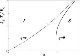
Figure 1: Phase diagram for the SC model without charge frustration (solid line) and with charge frustration $q=e$ (dashed line). $\alpha$ stands for the ratio $zE_{J}/4E_{C}$. The I and S indicate, respectively, insulating and superconducting phase.

We conclude this Section observing that the phase boundary line obtained within the mean-field approximation in the path-integral approach is $1/\alpha=g(q,y)$ with vanotterlo93 ; grignani00

$$g(q,y)=\frac{\sum_{n}e^{-\frac{4}{y}(n+\frac{q}{2e})^{2}}\frac{1}{1-4(n+\frac{q}{2e})^{2}}}{\sum_{m}e^{-\frac{4}{y}(m+\frac{q}{2e})^{2}}}.$$ (22)

Equation (22) coincides with Eqs. (15) and (17) for $q=e$ and $q=0$, respectively.

III Capacitive Disorder

In practical realizations of Josephson devices fazio01 , one has to deal with disorder caused by offset charge defects in the junctions or in the substrate krupenin00 . Random offset charges cannot be made to vanish by using a gate for each superconducting island since, in large arrays, too many electrodes would be necessary, making impossible the cooling of the system at the desired temperatures. In Ref. lafarge95 it was observed a sensible variation ($\sim 40\,\%$) of the resistance between the unfrustrated and the fully frustrated array. Moreover, it may also happen that the network’s parameters are not uniform across the whole array: despite recent advances in fabrication techniques, variation of junction parameters associated to the shape of the islands can be also of $20\,\%$ fazio01 . Thus, it is relevant in many practical situations to study JJA’s also with randomly distributed self-capacitances: this corresponds to have a random diagonal charging energy mancini03 ; alsaidi03 .

In this Section, we shall determine the finite temperature phase diagram of JJA’s with capacitive disorder (i.e., with random offset charges and/or random self-capacitances). To derive the phase boundary between the insulating and the superconducting phase, we shall use the mean-field approach for quantum JJA’s with offset charges and diagonal capacitance matrices reviewed in the previous Section. One has to impose now the self-consistency condition with a double average: the quantum average and the one over the disorder.

As we shall see, charge disorder supports superconductivity; furthermore, the relative changes of the insulating and superconducting regions of the phase diagram depend crucially on the weights of the $\delta$-like charge probability distribution. In the physical relevant situation of two charge distributions peaked at the values $q=0$ and $q=e$, increasing the frustrated weight favors the superconducting phase. Also the randomness of the self-capacitances leads to remarkable effects, namely, the superconducting phase increases with respect to the case where disorder is not present. In the following, we shall provide a quantitative analysis of these phenomena.

A pertinent extension of SCMFT in the presence of on-site disorder may be obtained introducing an order parameter averaged also over the disorder. In the following $\langle\cdots\rangle$ denotes only the quantum average while $[\cdots]_{av}$ an average over the random variables. The single-site Hamiltonians of Eq. (3) then become

$$H_{i}=-4E_{C}^{(i)}\frac{\partial^{2}}{\partial\varphi_{i}^{2}}-8iE_{C}^{(i)}\frac{q_{i}}{2e}\frac{\partial}{\partial\varphi_{i}}-zE_{J}\left[\langle\cos{\varphi}\rangle\right]_{av}\cos{\varphi_{i}}$$ (23)

where $E_{C}^{(i)}=e^{2}C_{ii}^{-1}/2$. The Hamiltonian (23) depends on a random variable $X$, which can be either $q_{i}$ or $E_{C}^{(i)}$. Thus, its eigenfunctions and eigenvalues depend either on $q_{i}$ or $E_{C}^{(i)}$:

$$H_{i}\,\psi_{n}(\varphi_{i};X)=E_{n}(X)\,\psi_{n}(\varphi_{i};X).$$ (24)

The self-consistency condition is given by

$$\left[\langle\cos{\varphi}\rangle\right]_{av}=\int dX\,P\left(X\right)\frac{\sum_{n}e^{-\beta E_{n}(X)}\langle\psi_{n}(X)|\cos\varphi|\psi_{n}(X)\rangle}{\sum_{n}e^{-\beta E_{n}(X)}}$$ (25)

where $P\left(X\right)$ is the probability distribution of $X$.

The phase boundary line is obtained from Eq. (25) by requiring $\left[\langle\cos{\varphi}\rangle\right]_{av}$ to be small and by keeping only terms proportional to it. The self-consistency condition yields a mean-field phase boundary line in agreement with the results obtained by the path-integral approach mancini03 . The low temperature behavior, obtained by a pertinent extrapolation of our finite $T$ results, is consistent with the phase diagram obtained in Ref. fisher89 (see Ref. mancini03 ).

III.1 Random Offset Charges

In this Section we shall study JJA’s at finite temperature with random charge frustration. One assumes that the offset charges are independently distributed according to a probability distribution given by a sum of $\delta$-like distributions

$$P(q_{i})=\sum_{n}p_{n}\,\delta(q_{i}-ne)$$ (26)

with $\sum_{n}p_{n}=1$. This corresponds to a random distribution of charges which are integer multiples of $e$ and, actually, this is the most realistic situation for a random distribution. Inserting the probability distribution (26) in Eq. (25), one has

$$\frac{1}{\alpha}=\int dq\sum_{n}p_{n}\,\delta(q-ne)g(q,y)=\sum_{odd}p_{n}\,g(ne,y)+\sum_{even}p_{n}\,g(ne,y)$$ (27)

where $\sum_{odd}$ ($\sum_{even}$) is a sum restricted to odd (even) integer.

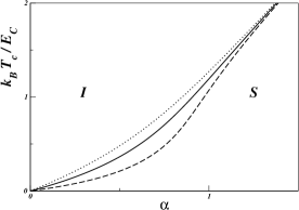
Figure 2: Phase diagram for random offset charges with the probability distribution given by Eq. (26). In the plot we take $p_{e}=1/4$ (dashed line), $1/2$ (solid line), and $3/4$ (dotted line).

Since the thermodynamical properties of the system are invariant under the shift $q\to q+2ne$, one should note that $g(q+2ne,y)=g(q,y)$, where $n$ is an integer. As a consequence, Eq. (27) leads to

$$\frac{1}{\alpha}=p_{0}\,g(0,y)+p_{e}\,g(e,y)$$ (28)

where $p_{0}=\sum_{even}\,p_{n}$ ($p_{e}=\sum_{odd}p_{n}$) is the probability that the offset charge $q$ is an even (odd) integer multiple of $e$. The results obtained from Eq. (27) with the probability distribution (26) are displayed in Fig. 2, where we plot the phase boundary line for $p_{e}=1/4,\>1/2,\>3/4$. One observes that increasing $p_{e}$ leads to an enlargement of the superconducting phase. It is worth noting that applying the SCMFT approximation with the probability distribution (26) it is possible to find exactly the same result obtained in a path-integral approach for a JJA model with diagonal capacitance matrices mancini03 .

III.2 Random Self-Capacitances

In this Section we shall study the finite temperature phase diagram of JJA’s with uniform charge frustration $q$ and random self-capacitances $C_{ii}$ with average $C_{0}$. Correspondingly, the average charging energy is $E_{C}^{0}=e^{2}/2C_{0}$. It is useful to define the charging energy terms $U_{ii}=8E_{C}^{(i)}$ and $U_{0}=8E_{C}^{0}$; averaging the self-consistency equation (25) over the random variables $U_{ii}$, the equation for the phase boundary becomes

$$\frac{1}{\alpha}=\int_{0}^{\infty}dU\>\frac{P(U)}{U}\>g(q,U,y)$$ (29)

where now $\alpha=2zE_{J}/U_{0}$, $y=8k_{B}T_{c}/U_{0}$ and $U=U_{ii}/U_{0}$. Equation (29) can be also obtained by using the path-integral approach mancini03 . The function $g(q=e,U,y)$ is given by

$$g(q=e,U,y)=\frac{\frac{4U+y}{4y}\>e^{-U/y}+\sum\limits_{n=1}^{\infty}\frac{1}{1-4(n+1/2)^{2}}\>e^{-(4U/y)(n+1/2)^{2}}}{e^{-U/y}+\sum\limits_{m=1}^{\infty}e^{-(4U/y)(m+1/2)^{2}}},$$ (30)

whereas the function $g(q=0,U,y)$ is given by

$$g(q=0,U,y)=\frac{\sum\limits_{n=-\infty}^{\infty}e^{-4U/y}\frac{1}{1-4n^{2}}}{\sum\limits_{m=-\infty}^{\infty}e^{-(4U/y)m^{2}}}.$$ (31)

If one, for instance, considers a bimodal distribution of the $U$’s, then

$$P(U)=p\>\delta(U_{1}-U)+(1-p)\>\delta(U_{2}-U),$$ (32)

where $U_{1}$ and $U_{2}$ are positive numbers. Inserting the probability distribution (32) in Eq. (29), one gets:

$$\frac{1}{\alpha}=p\,\frac{1}{U_{1}}\,g(q,U_{1},y)+(1-p)\,\frac{1}{U_{2}}\,g(q,U_{2},y).$$ (33)

The phase boundary line given by Eq. (33) is plotted in Fig. 3. One observes that, when $q=0$, the superconducting phase increases in comparison to the nonrandom case: this is due to the factors $1/U_{1}$ and $1/U_{2}$ in Eq. (33), which make larger the contribution of junctions with charging energies less than $U_{0}$. The increase of the superconducting phase is thus due to a decrease of the effective value of the charging energy. This phenomenon is largely independent from the specific choice of the distribution mancini03 .

It is pertinent to observe that, when $q=e$ (maximum frustration induced by the external offset charges), the randomness does not modify considerably the phase diagram. This should be compared with the unfrustrated case ($q=0$), where randomness sensibly affects the phase diagram.

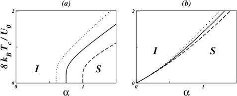
Figure 3: Phase diagram in the $T_{c}-\alpha$ plane for random diagonal charging energies distributed according to Eq. (32) and uniform offset charge $q=0$ (a), $q=e$ (b). $U_{0}$ is the average charging energy. We take $U_{1}=1/2$ and $U_{2}=3/2$, while $p$ is $1/4$ (dashed line), $1/2$ (solid line) and $3/4$ (dotted line).

IV Concluding Remarks

In this paper, we reviewed the use of the self-consistent mean-field theory to analyze the effects induced by offset charges on the finite temperature phase diagram of Josephson junction arrays.

We reviewed, for a diagonal Coulomb interaction matrix, the explicit derivation of the equation for the phase boundary line between the insulating and superconducting phase. The resulting phase diagram is drawn for a uniform offset charge distribution $q$: with $q=e$, the superconducting phase increases with respect to $q=0$, and the model exhibits superconductivity for all the values of $\alpha=zE_{J}/4E_{C}$. An offset charge $q=e$ tends therefore to decrease the charging energy and thus favors the superconducting behavior even for small Josephson energy $E_{J}$.

Using a pertinent extension of the self-consistent mean-field approach, we obtained here also the phase diagram at finite temperature of JJA’s with capacitive disorder. For a random distribution of offset charges which are integer multiples of $e$ one has that the superconducting phase increases in comparison with the unfrustrated case. For arrays with random charging energies, the superconducting phase increases with respect to the situation in which all self-capacitances are equal.

It is comforting to see that our mean-field analysis provides results which are in very good agreement with those obtained by Quantum Monte Carlo simulations alsaidi03_2 for most of the phase diagram.

References

- (1) R. F. Voss and R. A. Webb, Phys. Rev. B 25, 3446 (1982); R. A. Webb, R. F. Voss, G. Grinstein, and P. M. Horn, Phys. Rev. Lett. 51, 690 (1983).
- (2) E. Simànek, Inhomogeneous Superconductors, Oxford University Press, New York, 1994.
- (3) R. Fazio and H. van der Zant, Phys. Rep. 355, 235 (2001).
- (4) E. Roddick and D. Stroud, Phys. Rev. B 48, 16 600 (1993).
- (5) G. Luciano, U. Eckern and J. G. Kissner, Europhys. Lett. 32, 669 (1995); G. Luciano, U. Eckern, J. G. Kissner, and A. Tagliacozzo, J. Phys.: Condens. Matter 8, 1241 (1996).
- (6) A. I. Larkin and L. I. Glazman, Phys. Rev. Lett. 79, 3736 (1997).
- (7) M. Y. Choi, S. W. Rhee, M. Lee, and J. Choi, Phys. Rev. B 63, 094516 (2001).
- (8) C. Bruder, R. Fazio, A. Kampf, A. van Otterlo and G. Schön, Phys. Scri. 42, 159 (1992).
- (9) A. van Otterlo, K. H. Wagenblast, R. Fazio and G. Schön, Phys. Rev. B 48, 3316 (1993).
- (10) G. Grignani, A. Mattoni, P. Sodano, and A. Trombettoni, Phys. Rev. B 61, 11 676 (2000).
- (11) W. A. Al-Saidi and D. Stroud, cond-mat/0310047.
- (12) M. C. Diamantini, P. Sodano, and C. A. Trugenberger, Nucl. Phys. B 50 (1995); F. Cooper, P. Sodano, A. Trombettoni, and A. Chodos, Phys. Rev. D 68, 045011 (2003).
- (13) F. P. Mancini, P. Sodano, and A. Trombettoni, Phys. Rev. B 67 014518 (2003).
- (14) F. P. Mancini, P. Sodano, and A. Trombettoni, in New Developments in Superconductivity Research, edited by R. S. Stevens, Nova Science Publishers, New York, 2003, pg. 31.
- (15) M. P. A. Fisher, P. B. Weichman, G. Grinstein, and D. S. Fisher, Phys. Rev. B 40, 546 (1989).
- (16) E. Simànek, Solid State Commun. 31, 419 (1979).
- (17) M. Abramowitz and I. A. Stegun, Handbook of Mathematical Functions, Dover, New York, 1964.
- (18) Z. X. Wang and G. R. Guo, Special Functions, World Scientific, Singapore, 1989.
- (19) M. V. Simkin, Physica C 267, 161 (1996).
- (20) K. K. Likharev and A. B. Zorin, J. Low. Temp. Phys. 59, 347 (1985).
- (21) G. Schön and A. D. Zaikin, Physica, 152 B, 203 (1988).
- (22) E. Simànek, Phys. Rev. B 22, 459 (1980); Phys. Rev. B 23, 5762 (1981); Phys. Rev. B 32 500 (1985).
- (23) V. A. Krupenin, D. E. Presnov, A. B. Zorin, and J. Niemeyer, J. Low Temp. Phys. 118, 287 (2000).
- (24) P. Lafarge, J. J. Meindersma, J. E. and Mooji, in Macroscopic Quantum Phenomena and Coherence in Superconducting Networks, edited by C. Giovanella, and M. Tinkham, World Scientific, Singapore, 1995, pg. 94.
- (25) W. A. Al-Saidi and D. Stroud, Phys. Rev. B 67, 024511 (2003).