Transmission properties of a single metallic slit: From the subwavelength regime to the geometrical-optics limit

Abstract

In this work we explore the transmission properties of a single slit in a metallic screen. We analyze the dependence of these properties on both slit width and angle of incident radiation. We study in detail the crossover between the subwavelength regime and the geometrical-optics limit. In the subwavelength regime, resonant transmission linked to the excitation of waveguide resonances is analyzed. Linewidth of these resonances and their associated electric field intensities are controlled by just the width of the slit. More complex transmission spectra appear when the wavelength of light is comparable to the slit width. Rapid oscillations associated to the emergence of different propagating modes inside the slit are the main features appearing in this regime.

I Introduction

After the appearance of the experiment of Ebbesen et al. Ebbesen showing extraordinary optical transmission through a 2D array of subwavelength holes perforated in a thick metallic film, there has been a renewed interest in analyzing the optical properties of its 1D analog, an array of subwavelength slits Schroter ; Treacy ; Porto ; Astilean ; Sambles1 ; Collin ; Cao ; Barbara ; Garcia-Vidal1 . More recently, resonant transmission properties of a single subwavelength slit in a thick metallic screen have been analyzed both theoretically Takakura and experimentally Sambles2 ; Sambles3 ; Sambles4 . However, all these works consider the subwavelength regime. To the best of our knowledge, the study of the crossover between this regime and the geometrical-optics limit is still lacking.

In this work, we explore how the contribution to the transmission current of the different modes inside a single slit evolves as a function of the incident angle and the slit width. To get physical insight, we apply a formalism based on a modal expansion of the electromagnetic fields already proposed in an equivalent problem Martin-Moreno ; Garcia-Vidal2 . As we are interested in overall transmission behavior rather than in precise numerical comparison with experiments, we assume infinite conductivity for the metallic regions. Note, however, this approximation provides results of at least semi-quantitative value for good metals, such as silver or gold, if the dimensions of the structure are several times larger than the skin depthGarcia-Vidal1 . A bonus of using perfect metal boundary conditions is that all theoretical results are directly exportable to other frequency regimes, simply by scaling appropriately the geometrical parameters defining the structure.

This paper is organized as follows. In Sec. II we describe the theoretical formalism. This approach is applied to the subwavelength regime in Sec. III, where a comparison with available experimental data is also given. In addition, Sec. III presents two applications of a single subwavelength slit based on its characteristic resonant behavior. In Sec. IV we analyze the crossover between the subwavelength and the geometrical-optics limits. Finally, in Sec. V we summarize our results.

II Theoretical framework

In this work we are interested in the scattering process between a plane wave and the structure sketched in Fig. 1, i.e., a single metallic slit in a thick metal screen. Due to the translational invariance of the system along the $y$ axis, it is possible to write the vectorial Maxwell equations as two decoupled differential equations, one of them corresponding to s-polarization (electric field, ${\bf E}$, parallel to $y$ axis) and another corresponding to p-polarization (magnetic field, ${\bf H}$, parallel to $y$ axis). The case of s-polarization has been throughly analyzed in Schouten . Here, we concentrate on p-polarized light in which resonant transmission properties have been reported. For this polarization, the response of the structure can be solved by finding the solutions of the following equation

$$\nabla\left[{\frac{1}{\epsilon({\bf r})}}\nabla H_{y}({\bf r})\right]+{\frac{\omega^{2}}{c^{2}}}H_{y}({\bf r})=0$$ (1)

where we have assumed a harmonic time dependence of angular frequency $\omega$. $H_{y}({\bf r})$ is the y-component of the magnetic field and ${\bf r}=(x,z)$. $\epsilon({\bf r})$ defines the spatial distribution of the dielectric constant.

Once we know the field $H_{y}({\bf r})$, the spatial components of the electric field can be obtained from

$$E_{x} = -{\frac{i}{k_{0}\epsilon({\bf r})}}\frac{\partial H_{y}}{\partial z}\;,{\rm and},$$ (2)

$$E_{z} = \frac{i}{k_{0}\epsilon({\bf r})}\frac{\partial H_{y}}{\partial x}$$ (3)

To solve Eq. (1) it is convenient to divide the space into three different regions (labelled as I,II and III in Fig. 1). The magnetic field $H_{y}$ can be expressed in regions I and III as a superposition of propagating and evanescent plane waves as

$$H_{y}^{I}({\bf r}) = H_{y}^{inc}({\bf r})+\int_{-\infty}^{\infty}{\rm d}k\>\rho(k)\>\exp[i(kx-k_{z}z)]$$ (4)

$$H_{y}^{III}({\bf r}) = \int_{-\infty}^{\infty}{\rm d}k\>\tau(k)\>\exp[i(kx+k_{z}z)]$$ (5)

where $k_{z}=\sqrt{k_{0}^{2}-k^{2}}$, being $k_{0}$ the modulus of the wavevector of the incident plane wave. The coefficients $\rho(k)$ and $\tau(k)$ are the transmission and reflection amplitudes, respectively. The incident field is given by $H_{y}^{inc}({\bf r})=\exp[i(k_{0x}x+k_{0z}z)]$, being $k_{0x}$ and $k_{0z}$ the projections of the incident wavevector on the x and z axis, respectively (see Fig. 1).

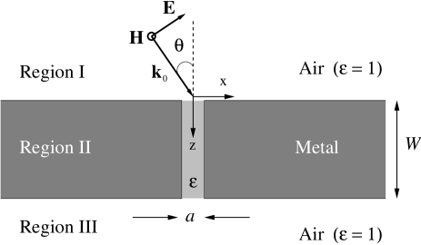
Figure 1: Schematic plot of the structure under study. Dark grey corresponds to metallic regions while light gray corresponds to a region defined by a homogeneous dielectric constant $\epsilon$. Both the reference system and the geometrical parameters that define this system are plotted.

Inside the slit, the solution can be expanded as a sum of the eigenmodes of a waveguide

$$H_{y}^{II}({\bf r})=\sum_{m=0}^{\infty}\>[A_{m}\>\exp(i\beta_{m}z)+\>B_{m}(-i\beta_{m}z)]\>\phi_{m}(x)$$ (6)

where $\beta_{m}=[k_{0}^{2}\epsilon-(m\pi/a)^{2}]^{\frac{1}{2}}$ and the function $\phi_{m}(x)=(2/\sqrt{a})\cos[m\pi/a(x+a/2)]$ corresponds to the solution of Eq. (1) within the slit, assuming perfect metal boundary conditions at $x=\pm a/2$. A homogeneous material without absorption and characterized by a dielectric constant $\epsilon$, is considered inside the slit (light gray area in Fig. 1). By allowing $\epsilon$ to vary we plan to check the reliability of a single slit as a fluidics detector.

By applying the corresponding matching conditions to both $H_{y}$ and $E_{x}$ at $z=0$ and $z=W$ and proyecting the resulting equations on waveguide modes and plane waves, we obtain a system of linear equations with the set of coefficients $\{A_{m},B_{m}\}$ as unknowns. We find that this problem is equivalent to that reported very recently in Refs. 15 and 16. In other words, the scattering problem studied in this paper is equivalent to consider a finite set of indentations with only one relevant mode inside each indentation. Therefore, to obtain more physical understanding of the mechanisms that take part in this scattering problem, it is convenient to change the set of variables $\{A_{m},B_{m}\}$ by the new set $\{E_{m}^{I},E_{m}^{O}\}$ defined by

$$E_{m}^{I} = \frac{\beta_{m}}{k_{0}\epsilon}(A_{m}-B_{m})$$ (7)

$$E_{m}^{O} = \frac{\beta_{m}}{k_{0}\epsilon}[A_{m}\exp{(i\beta_{m}W)}-B_{m}\exp{(-i\beta_{m}W)}]$$ (8)

The set of equations to solve for the amplitudes $\{E_{m}^{I},E_{m}^{O}\}$ can be expressed as

$$(f_{m}+g_{mm})E_{m}^{I}+\sum_{m^{\prime}\neq m}g_{mm^{\prime}}E_{m^{\prime}}^{I}+g_{m}^{v}E_{m}^{O} = I_{m}$$ (9)

$$(f_{m}+g_{mm})E_{m}^{O}+\sum_{m^{\prime\prime}\neq m}g_{mm^{\prime\prime}}E_{m^{\prime\prime}}^{O}+g_{m}^{v}E_{m}^{I} = 0$$ (10)

We can interpret the equations (9) and (10) as follows. The $m$-th mode has two associated field amplitudes, one of them ($E_{m}^{I}$) corresponds to the scattering events that take place at the input surface of the slit, while the another amplitude ($E_{m}^{O}$) is related to the output surface. Each amplitude is determined as the result of different scattering processes between all modes. Now, we pass to analyze in detail the different terms appearing in the set of equations (9) and (10).

$I_{m}$ is the overlap integral between the incident plane wave and $m$-th mode

$$I_{m}=2\int_{\frac{-a}{2}}^{\frac{a}{2}}\textrm{dx}\>\phi_{m}(x)\>\exp(ik_{0}\sin\theta\>x)$$ (11)

Modes inside the slit are coupled through $g_{mm^{\prime}}$

$$g_{mm^{\prime}}=\int_{\frac{-a}{2}}^{\frac{a}{2}}\int_{\frac{-a}{2}}^{\frac{a}{2}}\textrm{dx}\>\textrm{dx'}\phi_{m}^{*}(x)\>\phi_{m^{\prime}}(x^{\prime})\>G({\bf{\hat{x}}r},{\bf{\hat{x}^{\prime}}r^{\prime}})$$ (12)

The function $G({\bf r},{\bf r^{\prime}})=(\pi/\lambda)H_{0}^{(1)}(k_{0}|{\bf r}-{\bf r^{\prime}}|)$ is the two-dimensional Green’s function corresponding to the vacuum, being $H_{0}^{(1)}(x)$ the Hankel function of the first kind. The unitary vectors ${\bf{\hat{x}}}$ and ${\bf{\hat{x}^{\prime}}}$ correspond to x and x’ axis, respectively. Notice that the propagator $g_{mm^{\prime}}$ does not depend on the dielectric constant inside the slit but on the dielectric constant of the material outside, i.e., the coupling between modes takes places through the external medium.

Amplitude of the $m$-th mode is inversely proportional to $f_{m}+g_{mm}$, where $f_{m}$ is the associated admittance of that mode and $g_{mm}$ is the self-interaction term.

$$f_{m}=k_{0}\>\epsilon\>\gamma_{m}\frac{\exp(-i\beta_{m}W)+\exp(i\beta_{m}W)}{\beta_{m}[\exp(-i\beta_{m}W)-\exp(i\beta_{m}W)]}$$ (13)

where $\gamma_{m}$ comes from the normalization factors of the wavefield inside the slit and it is equal to 1 if $m=0$ and 1/2 if $m\neq 0$.

Amplitude of the $m$-th mode corresponding to the input surface is coupled to its counterpart in the output side through $g_{m}^{v}$

$$g_{m}^{v}=k_{0}\>\epsilon\>\gamma_{m}\frac{2}{\beta_{m}(\exp[i\beta_{m}W)-\exp(-i\beta_{m}W)]}$$ (14)

It can be proved that in the case of a non uniform slit, modes with different $m$ values are also coupled.

It is possible to write the Fourier coefficients $\rho(k)$ and $\tau(k)$ as a function of $\{E_{m}^{I},E_{m}^{O}\}$

$$\rho(k) = \delta(k-k_{0x})-\sum_{m=0}^{\infty}E_{m}^{I}\>S_{m}(k)\>\>\textrm{and}$$ (15)

$$\tau(k) = \sum_{m=0}^{\infty}E_{m}^{O}\>S_{m}(k)$$ (16)

where

$$S_{m}(k)=\frac{1}{2\pi\sqrt{1-(k/k_{0})^{2}}}\int_{-\frac{a}{2}}^{\frac{a}{2}}\textrm{dx}\>\phi_{m}(x)\>\exp(-ikx)$$ (17)

Therefore the field $H_{y}$ in air regions can be obtained from

$$H_{y}^{I}({\bf r}) = H_{y}^{0}({\bf r})+\sum_{m=0}^{\infty}(-E_{m}^{I})\>G_{m}({\bf r})$$ (18)

$$H_{y}^{III}({\bf r}) = \sum_{m=0}^{\infty}E_{m}^{O}\>G_{m}({\bf r})$$ (19)

where we define $H_{y}^{0}({\bf r})=2\cos(k_{0z}z)\exp(ik_{0x}x)$ and

$$G_{m}({\bf r})=\int_{-\frac{a}{2}}^{\frac{a}{2}}\textrm{dx'}\>\phi_{m}(x^{\prime})\>G(\bf{r},\bf{r^{\prime}})$$ (20)

with $\bf{r}$=(x,z) and being ${\bf r^{\prime}}=(x^{\prime},0)$ for the reflection region ($z<0$) and ${\bf{r^{\prime}}}=(x^{\prime},W)$ for the transmission region ($z>W$).

Equations (18) and (19) have a clear physical interpretation: scattered fields outside the sample are the result of the sum of those corresponding to a flat dielectric-metal interface $[H_{y}^{0}({\bf r})]$ and the contribution from each mode within the slit considered as an individual scatterer.

We can define the transmission current in the propagation direction as

$$J_{z}=\int_{-\infty}^{\infty}\textrm{dx}\>\Re\{[{\bf E^{*}(r)}\times{\bf H(r)}]_{z}\}$$ (21)

If we normalize the transmission of the system ($T$) to the flux of energy that impinges on the slit we can write for region III

$$T=\frac{1}{a}\>\Re(\sum_{m,m^{\prime}=0}^{\infty}E_{m^{\prime}}^{O}E_{m}^{O*}\>g_{mm^{\prime}})$$ (22)

As no absorption is present in the structure, current is conserved and the transmittance can be then alternatively and more easily evaluated inside the slit (region II)

$$T=\frac{1}{a}\>\Re(\sum_{m}^{\infty}E_{m}^{I*}E_{m}^{O}\>g_{m}^{v})$$ (23)

III Transmission in the subwavelength regime

First of all, we consider the transmission properties in the subwavelength limit, i.e., when $\lambda/a\gg 1$. In order to compare our numerical results with available experimental data, we begin by asumming $W=28.2$ mm and the same range of wavelengths considered in Ref. 12.

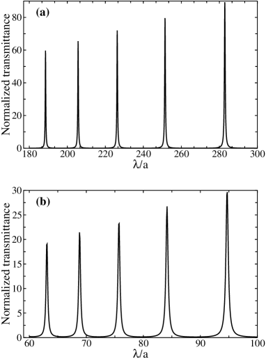
Figure 2: Transmittance of a metallic single slit as a function of the wavelength of the incident radiation, computed with the same W=28.2 mm and two different values of $a$, 25 $\mu$m (a) and 75 $\mu$m (b). Notice that the wavelength range considered is the same in the two panels. Normal incidence and $\epsilon$=1 inside the slit is assumed.

Figure 2 shows the transmittance in two different ranges of $\lambda/a$ within the subwavelength regime [in Fig. 2(a) we take $a$=25 $\mu$m while in Fig. 2(b) we consider $a$=75 $\mu$m]. In this figure we assumed normal incidence and $\epsilon$=1 within the slit. In the subwavelength regime, only the propagating $m=0$ mode has a non-negligible contribution to the transmittance. Then, for this particular case, the set of equations (9)-(10) converts into a system of two linear equations with a solution for $E_{0}^{O}$

$$E_{0}^{O}=-\frac{g_{0}^{v}I_{0}}{(f_{0}+g_{00})^{2}-g_{0}^{v2}}$$ (24)

It is then clear that the resonant transmission peaks observed in Fig.2 are associated with the zeroes of the denominator of Eq. (24). In the strict limit $a/\lambda\rightarrow 0$, $g_{00}$ goes to zero [as $a/\lambda\>Ln(a/\lambda)$] and resonant transmission appears at the condition $f_{0}=\pm g_{0}^{v}$, which straightforward algebra shows equivalent to the usual Fabry-Perot resonant condition $sin(k_{0}\sqrt{\epsilon}W)=0$. When $a/\lambda$ is small but not zero, the transmission peaks are shifted and broadened due to the non-negligible contribution of the real and imaginary part of $g_{00}$, respectively. Therefore, we can say that a subwavelength metallic slit behaves basically as a Fabry-Perot interferometer made of high reflective plates. Following with this analogy, it can be shown that when the slit width increases, the modulus of the reflection coefficients at the edges of the slit decreases, and therefore the efficiency of the system as a interferometer becomes poorer.

The numerical results shown in Fig. 2(b) are in agreement with experimental data published by Yang and SamblesSambles2 . However, it is worth noticing that for this case the expression obtained in Ref. 11, where only the leading terms in $a/\lambda$ are considered, overestimates (about 10%) the shift of resonant peaks from the usual Fabry-Perot resonant condition, $\sin(k_{0}\sqrt{\epsilon}W)=0$, showing that the asymptotic $a/\lambda\to 0$ limit is reached very slowly.

Another interesting feature observed in the subwavelength regime is that transmittance does not depend on the angle of incidence. This can be easily understood by looking at Eq.(11). In this expression, the only quantity that depends on $\theta$ is $I_{0}$

$$I_{0}(\theta)=2\>\textrm{sinc}\left[\pi\left(\frac{a}{\lambda}\right)\sin\theta\right]$$ (25)

where $sinc(x)=sin(x)/x$. If $a/\lambda$ is small enough the dependence of this coupling on the incident angle is negligible as $sinc\approx 1$, independent on $\theta$.

Figure 3: Contour plot of the electric field intensity of a single metallic slit defined by $a$=40 $\mu$m, $W$=1 mm. Incident radiation with $\lambda$=409 $\mu$m and $\theta$=0 is assumed. Red (blue) means maximum (minimum) field intensity.

Notice that, as it was mentioned before, we are normalizing the transmittance to the energy that reaches the slit. Therefore, since the total transmission in the resonant peaks for $a$=25$\mu$m is about three times that of $a$=75 $\mu$m, we can deduce that the energy flux collected by the slit at resonances is approximately the same for any value of $a$. This extraordinary property also implies that the electric field intensity inside the slit satisfies a $1/a$ dependence, and therefore, huge enhancements of the electric field intensity can be achieved just by reducing the slit width. However, as a leaky standing wave is excited within the slit, only a periodic set of regions will undergo the enhancement of the electric field intensity, as is shown in the contour plot of Fig. 3, where we have considered a representative example with $a$=40 $\mu$m and $W$=1 mm. Therefore, introducing a suitable non-linear medium inside the slit would produce a periodic modulation of the refractive index in the direction of propagation. In other words, an one-dimensional photonic crystal is formed by the electromagnetic radiation at the resonant frequencies.

It is also worth commenting that, as illustrated in Fig.2, the linewidth of the transmission resonances decreases when the slit width is reduced. This property allows us to measure the dielectric constant of small amounts of material filling the slit through the variation of the resonant wavelengths with $\epsilon$, as has been suggested by Yang and SamblesSambles3 ; Sambles4 . In this paper, we study the accuracy of this kind of structure to work as a high-sensitivity microfluidics detector. Within this context, very recently, changes in transmission properties of photonic crystals have been proposed as a way to identify certain very small quantities of fluids Topolancik . Here, we analyze a simple but functional alternative to this approach. A small amount of a fluid can be guided to flow within the slit and just by recording the location of the transmission resonances, an estimation of the dielectric constant of the material can be obtained. To prove this proposal, Fig. 4a shows a contour plot of the transmittance as a function of the wavelength and the dielectric constant inside the slit. The efficiency of this system is shown in of Fig. 4b where the same two fluids considered in Ref. 18 are assumed to fill the slit, i.e., $\epsilon$=1.8978 (isopropanol) and $\epsilon$=2.2506 (xylene). As can be seen from this figure, the two peaks are well separated and, in principle, with a slit with the geometrical parameters we have used in this simulation, this device could distinguish whether isopropanol or xylene are filling the slit. If we were interested in characterizing two fluids with more similar dielectric constants, we could obtain even higher resolution in the transmission resonances by just reducing the slit width. As commented previously, this device also is expected to work in the optical regime allowing then to characterize nanometric amounts of fluids.

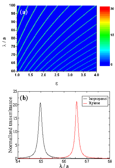
Figure 4: (a) Contour plot of the transmittance as a function of the wavelength and the dielectric constant inside the slit. Geometrical parameters as in Fig. 2(b) are assumed. (b) Comparison of the transmittance obtained with $\epsilon$=1.8978 (black line) and $\epsilon$=2.2506 (red line).

IV Crossover between the subwavelength regime and the geometrical-optics limit

In the previous sections we have found no dependence of the normalized transmittance with the angle of incidence in the extremely subwavelength limit. When the slit width increases, the dependence of the transmittance on incident angle becomes important. If $a/\lambda$ is still small enough that only the first mode ($m$=0) contributes appreciably to the transmission, the coupling with the external plane wave is governed by $I_{0}(\theta)$ [see Eq.(25)]. This is the case of the transmittance spectrum plotted in Fig. 5(a), where we assume $a$=1.25 mm. As shown in this figure, transmittance is maximum for $\theta=0^{\circ}$ and decreases very slowly when $\theta$ is increased.

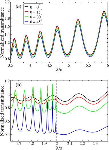
Figure 5: Transmittance computed with W=28.2 mm and (a) a=1.25 mm and (b) a=2.75 mm. Black, red, green and blue correspond to $\theta$ =0^∘, 15^∘, 30^∘, and 45^∘, respectively.

By increasing $a$, several eigenmodes with $m>0$ (both evanescent and propagating) start having a non-negligible contribution to the transmittance. The coupling of these $m>0$ modes with the external radiation and between them is given by $I_{m}$ and $g_{mm^{\prime}}$, respectively. An example of this behavior is shown in Fig. 5(b), where $a$=2.75 mm. As can be seen in this figure, when a slit mode changes its character from evanescent to propagating (dashed line in Fig. 5(b) shows the wavelength where $m=1$ becomes propagating, $\lambda=2a$), resonant transmission properties change dramatically. Interestingly, this change is not observed for $\theta=0^{\circ}$. This is due to the fact that $I_{m}(\theta=0^{\circ})=0$ for $m>0$ and $g_{0m}=0$ for $m$ odd. Then for this particular case of $\theta=0^{\circ}$ and for this range of wavelengths, transmission is governed by mode $m=0$. Similar abrupt changes, at wavelengths where eigenmodes with higher values of $m$ become propagating, have been also theoretically predicted for the transmission spectrum of light impinging on a circular aperture made in a perfect metal screen Roberts ; deAbajo .

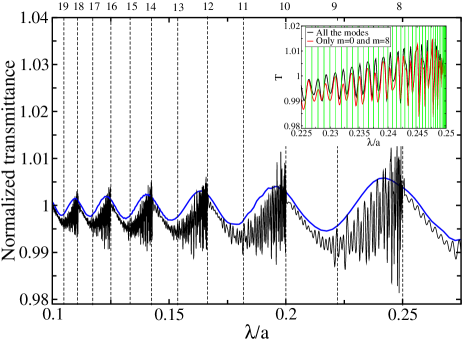
Figure 6: Main: transmittance computed with W=28.2 mm and a=2.75 mm. Dashed lines show the wavelengths where the corresponding mode (see labels on top) becomes propagating. Blue line corresponds to consider only the fundamental mode. Inbox: Comparison of the transmittance calculated taken into account all the modes (black line) and only m=0 and m=8 (red line). Vertical green lines show the wavelengths where the Fabry-Perot condition is fulfilled for m=8 (see text).

Now, let us focus in the interval $0.1<\lambda/a<0.275$. Solid black line in Fig. 6 shows the transmittance in this interval of wavelengths for $a$=2.75 mm. For the sake of simplicity, in this section we analyze only normal incidence. If $\theta\neq$0^∘ similar physical mechanisms are present. Dashed lines show the wavelengths where the corresponding mode changes it character from evanescent to propagating. First of all, notice that transmission peaks are associated to the emergence of propagating even modes and not to odd ones. This can be understood by realizing that, as commented before, for normal incidence, odd modes are uncoupled both to the external radiation and to the $m$=0 mode. Even modes, although uncoupled to the normal incident radiation, have an indirect illumination through their coupling with $m$=0 mode. In addition, this makes that the fundamental mode approximately gives the overall transmission envelope (see blue line in Fig. 6).

We have found that near the wavelength where the m-th mode (being m a even integer) changes its character from evanescent to propagating, i.e., at $\lambda/a=2/m$, transmission features are mainly governed by the contribution of only the mode m=0 and the m-th mode. In order to prove quantitatively this property, inbox of Fig. 6 shows the transmission in the neighborhood of the wavelength where m=8 becomes a propagating mode ($\lambda/a$=0.25). Black line in this figure shows the result considering all the modes within the slit, while red line shows the same calculation but now including only modes with $m$=0 and $m$=8 in Eqs. (9) and (10). We have found that $m$=0 gives the background of the transmittance while $m$=8 produces approximately the oscillatory behavior. These rapid oscillations of the spectrum can be explained by analyzing the $z$-component of the wavevector ($k_{z}$) associated to the corresponding eigenmode when this mode changes from evanescent to propagating. Within the range of wavelengths in which this change occurs, $k_{z}\rightarrow 0$ and then Fabry-Perot condition $sin(k_{z}\sqrt{\epsilon}W)=0$ is fulfilled for many wavelengths inside this interval, resulting in transmission peaks with a very small wavelength separation between them (see vertical green lines in inbox of Fig. 6). Finally, from Fig. 6 we can see how the amplitude of the transmittance oscillations decreases and tend to 1 when $\lambda/a\to 0$, as it is expected from geometrical optics.

V Summary

In this work, a formalism for analyzing the transmission properties of a single metallic slit under general conditions of angle of incidence and slit width has been presented.

First of all, we have carried out a comprehensive study of the subwavelength regime. We have discussed the appearance of transmission resonances associated to the excitation of slit waveguide modes. We have also discussed two possible devices based on the huge enhancement of the EM-fields inside the slit that accompanies the extraordinary transmission phenomenon: a non-linear device and a micro or nano-fluidics detector.

In addition, the behavior of the transmittance when the subwavelength limit is abandoned has been also analyzed. We have studied in detail how the geometrical optics limit ($T=1$) is recovered. In this regime, rapid oscillations in the transmission spectrum appear near the wavelength where a mode becomes propagating.

References

- (1) T.W. Ebbesen, H.J. Lezec, H.F. Ghaemi, T. Thio T, and P.A. Wolff, Nature (London) 391, 667 (1998).
- (2) U. Schroter and D. Heitmann, Phys. Rev. B 58, 15419 (1998).
- (3) M.M.J. Treacy, Appl. Phys. Lett. 75, 606 (1999).
- (4) J.A. Porto, F.J. García-Vidal, and J.B. Pendry, Phys. Rev. Lett. 83, 2845 (1999).
- (5) S. Astilean, Ph. Lalanne, and M. Palamaru, Opt. Comm. 175, 265 (2000).
- (6) H.E. Went, A.P. Hibbins, J.R. Sambles, C.R. Lawrence, and A.P. Crick, Appl. Phys. Lett. 77, 2789 (2000).
- (7) S. Collin, F. Pardo, R. Teissier, and J.L. Pelouard, Phys. Rev. B 63, 33107 (2001).
- (8) Q. Cao and Ph. Lalanne, Phys. Rev. Lett. 88, 57403 (2002).
- (9) A. Barbara, P. Quémerais, E. Bustarret, and T. López-Ríos, Phys. Rev. B 66, 161403(R) (2002).
- (10) F.J. García-Vidal and L. Martín-Moreno, Phys. Rev. B 66, 155412 (2002).
- (11) Y. Takakura, Phys. Rev. Lett. 86, 5601 (2001).
- (12) F. Yang and J.R. Sambles, Phys. Rev. Lett. 89, 63901 (2002).
- (13) F. Yang and J.R. Sambles, Appl. Phys. Lett. 81, 2047 (2002).
- (14) F. Yang and J.R. Sambles, J. Phys. D 35, 3049 (2002).
- (15) L. Martín-Moreno, F.J. García-Vidal, H.J. Lezec, A. Degiron, and T.W. Ebessen, Phys. Rev. Lett. 90, 167401 (2003).
- (16) F.J. García-Vidal, H.J. Lezec, T.W. Ebessen, and L. Martín-Moreno, Phys. Rev. Lett. 90, 213901 (2003).
- (17) H.F. Schouten, T.D. Visser, D. Lenstra, and H. Blok, Phys. Rev. E 67, 36608 (2003); H.F. Schouten, T.D. Visser, G. Gbur, D. Lenstra, and H.Blok, Opt. Express 11, 371 (2003).
- (18) J. Topolancik, P. Bhattacharya, J. Sabarinathan, and P.C. Yu, Appl. Phys. Lett. 82, 1143 (2003).
- (19) A. Roberts, J. Opt. Soc. Am. A 4, 1970 (1987).
- (20) F.J. García de Abajo, Opt. Express 10, 1475 (2002).