Fluctuations of entropy production in the isokinetic ensemble

Abstract

We discuss the microscopic definition of entropy production rate in a model of a dissipative system: a sheared fluid in which the kinetic energy is kept constant via a Gaussian thermostat. The total phase space contraction rate is the sum of two statistically independent contributions: the first one is due to the work of the conservative forces, is independent of the driving force and does not vanish at zero drive, making the system non-conservative also in equilibrium. The second is due to the work of the dissipative forces, and is responsible for the average entropy production; the distribution of its fluctuations is found to verify the Fluctuation Relation of Gallavotti and Cohen. The distribution of the fluctuations of the total phase space contraction rate also verify the Fluctuation Relation. It is compared with the same quantity calculated in the isoenergetic ensemble: we find that the two ensembles are equivalent, as conjectured by Gallavotti. Finally, we discuss the implication of our results for experiments trying to verify the validity of the FR.

Keywords: isokinetic ensemble, entropy production rate, fluctuation theorem, ensemble equivalence

I Introduction

A very important concept in the theory of out-of-equilibrium stationary states induced by the application of a driving force (temperature or velocity gradients, electric fields, etc.) to a system in contact with a thermal bath is that of entropy production rate gal1 ; gal2 . In usual nonequilibrium thermodynamics it is defined as the power dissipated by the driving force divided by the temperature of the bath evans :

$$\dot{\sigma}(t)=\frac{1}{T}\sum_{i}J_{i}(t)X_{i}(t)\ .$$ (1)

Here $X_{i}(t)$ is the driving force (e.g. the electrical field or the temperature gradient) and $J_{i}(t)$ its conjugated flux (the electrical current or the heat flux respectively).

The Probability Distribution Function (PDF) of the total entropy production over a time $\tau$ is defined as

$$P_{\tau}(\sigma)=P\left(\int_{0}^{\tau}dt\ \dot{\sigma}(t)=\sigma\right)\ .$$ (2)

If we set $k_{B}=1$, $\dot{\sigma}(t)$ has the dimension of an inverse time and $\sigma$ is dimensionless. Then, in the limit of large $\tau$, the function $P_{\tau}(\sigma)$ is expected to verify the Fluctuation Relation (FR) in the following form:

$$P_{\tau}(-\sigma)=e^{-\sigma}\ P_{\tau}(\sigma)\ ,$$ (3)

if $|\sigma/\langle\sigma\rangle|<C$, being $C$ a positive constant. Having fixed $C$, the correction at finite $\tau$ is of order one in the exponent of the right side of Eq. 3 (while $\sigma$ is of order $\tau$ if $\gamma\neq 0$). The FR states that the probability to observe a negative entropy production (over a large enough time interval) is exponentially smaller than the probability to observe the same value with positive sign. This relation has been first observed numerically in a sheared fluid ECM and subsequently proven to hold for reversible systems by Gallavotti and Cohen under the chaotic hypothesis, a strong chaoticity assumption for the dynamics of the system, leading to the demonstration of the Fluctuation Theorem (FT) GC . Gallavotti then showed that in the limit of small driving forces the FT implies the usual Green-Kubo relations and the Fluctuation-Dissipation Theorem GAL , thus clarifying the deep physical significance of Eq. 3. Despite the hypothesis of the FT are strictly verified only for very special systems, the FR has been shown to be valid for a large class of dissipative systems in very different conditions BGG ; BCL ; Kurchan ; LebSpo ; vulpiani ; GP . Some experimental attempts have also been done in order to check its validity for real systems ciliberto ; goldburg ; menon .

The verification of Eq. 3 in microscopic models for dissipative systems requires a microscopic definition of $\dot{\sigma}(t)$. In the case of conservative models, in which the phase space volume is conserved in absence of drive, the entropy production rate has been identified at the microscopic level with the phase space contraction rate ECM ; BGG ; BCL ; GP . One can ask if the same identification holds for models in which the phase space volume is not conserved even in absence of the driving force.

It has been conjectured by Gallavotti that, if the entropy production rate is properly defined, equivalence of ensembles should hold, in the sense that the FR must hold for a subsystem of the (big) dynamical system under consideration, at least for a large class of thermostatting mechanisms, including irreversible and stochastic ones gal1 ; gal2 ; gal_stat ; gal_fluid .

In this paper we will discuss two different models of thermostat, both mechanical and reversible (then, we will not discuss the problem of equivalence between reversible and irreversible thermostats), defining two different ensembles: the first one is constructed in order so that the total phase space contraction rate vanishes in equilibrium, while in the second one fluctuations of the total phase space contraction rate are present even in the limit of zero driving force, thus making the system non-conservative also in equilibrium. We will then discuss the equivalence of these ensemble and the possibility of identifying the entropy production rate with the phase space contraction rate when the latter is not vanishing in equilibrium.

II Two models of a mechanical thermostat

We consider a well known microscopic model for a sheared fluid defined by the SLLOD equations evans :

$$\begin{cases}&\dot{q}_{i}=\frac{p_{i}}{m}+\gamma y_{i}\hat{x}\ ,\\ &\dot{p}_{i}=F_{i}-\gamma p_{yi}\hat{x}-\alpha(p,q)p_{i}\ ,\end{cases}$$ (4)

where $F_{i}$ are conservative forces, $F_{i}=-\partial_{q_{i}}V(q)$. The terms proportional to $\gamma$ (the shear rate) impose to the liquid a flow along the $x$ direction with a gradient velocity field along the $y$ axis. In this model the driving force is the velocity gradient $\gamma$, and its conjugated flux is the $yx$ component of the stress tensor, $P_{yx}$. The function $\alpha(p,q)$ is a Gaussian thermostat, and can be defined in order to conserve either the total energy $H(p,q)=\sum_{i}\frac{p_{i}^{2}}{2m}+V(q)$ or the kinetic energy alone. The total phase space contraction rate for this system is given by:

$$\dot{\sigma}(p,q)=-\sum_{i}\left(\frac{\partial\dot{q}_{i}}{\partial q_{i}}+\frac{\partial\dot{p}_{i}}{\partial p_{i}}\right)=3N\alpha(p,q)+\sum_{i}\frac{\partial\alpha}{\partial p_{i}}p_{i}\ .$$ (5)

The second term is of order one in the case we will discuss, and will be neglected with respect to the first term.

II.0.1 Isoenergetic (or microcanonical) ensemble

Imposing the constraint $dH/dt=0$, one gets the following expression for $\alpha$:

$$\alpha_{H}(p,q)=-\gamma\frac{\sum_{i}(p_{xi}p_{yi}+mF_{xi}y_{i})}{\sum_{i}p^{2}_{i}}\ .$$ (6)

The expression for the phase space contraction rate is then:

$$\dot{\sigma}_{H}(p,q)=3N\alpha_{H}(p,q)=-\frac{\gamma P_{yx}(p,q)}{T(p)}\equiv\dot{\sigma}_{\gamma}(p,q)\ ,$$ (7)

where $T(p)=\frac{1}{3N}\sum_{i}\frac{p^{2}_{i}}{m}$ and $P_{yx}(p,q)=\sum_{i}(p_{xi}p_{yi}/m+F_{xi}y_{i})$ is the microscopic expression of the $yx$ component of the stress tensor evans . Note that in this case the phase space contraction rate is exactly equal to the microscopic expression of Eq. 1. From Eq. 7 we see that in the isoenergetic ensemble the phase space volume is conserved in equilibrium as $\dot{\sigma}_{H}$ is vanishing for $\gamma=0$. The behavior of the fluctuations of $\dot{\sigma}_{H}$ has been discussed in ECM where the validity of the FR for $P_{\tau}(\sigma_{H})$ was observed for the first time.

II.0.2 Isokinetic ensemble

If the temperature $T(p)$ has to be conserved instead of the total energy, one obtains the following expression for $\alpha$:

$$\alpha_{T}(p,q)=\frac{\sum_{i}p_{i}F_{i}-\gamma\sum_{i}p_{xi}p_{yi}}{\sum_{i}p^{2}_{i}}=\alpha_{H}(p,q)+\frac{\sum_{i}m\dot{q}_{i}F_{i}}{\sum_{i}p^{2}_{i}}\ ,$$ (8)

and the total phase space contraction rate is given by

$$\dot{\sigma}_{T}(p,q)=-\frac{\gamma P_{yx}(p,q)}{T(p)}+\frac{\sum_{i}\dot{q}_{i}F_{i}}{T(p)}=\dot{\sigma}_{\gamma}(p,q)+\dot{\sigma}_{c}(p,q)\ .$$ (9)

From the previous expression one sees that the total phase space volume contraction rate in the isokinetic ensemble is the sum of two different contributions: the first one ($\dot{\sigma}_{\gamma}$) is due to the work of the dissipative forces and has the same microscopic expression as in the isoenergetic ensemble (see Eq. 7); the second one ($\dot{\sigma}_{c}$) is the power dissipated by the conservative forces divided by the temperature. It is easy to see that it the second term can be also written as $\dot{\sigma}_{c}(p,q)=-T^{-1}(p)\frac{dV(q)}{dt}$; thus, it has zero average (because the total potential energy is constant in average). This term is present also in equilibrium ($\gamma=0$): then, in the isokinetic ensemble, the phase space volume is not conserved also in equilibrium, at variance to what happens in the isoenergetic ensemble. However, the two ensembles are known to be equivalent in equilibrium evans .

II.0.3 Ensemble equivalence in nonequilibrium

Having defined these two model of thermostat, two questions naturally arise:
1) One can ask if the proper definition of $\dot{\sigma}(t)$ (i.e. the one that verifies the FR) in the isokinetic ensemble is given by the total phase space contraction rate $\dot{\sigma}_{T}$ or by $\dot{\sigma}_{\gamma}$ alone;
2) Once a definition for the entropy production rate in the isokinetic ensemble has been chosen, one can compare the distribution of its fluctuation with the same quantity calculated in the isoenergetic ensemble, thus verifying if some kind of nonequilibrium ensemble equivalence holds gal1 ; gal2 .

To address this points, we will check numerically the validity of the following statements:
i) $\dot{\sigma}_{\gamma}$ and $\dot{\sigma}_{c}$ defined in Eq. 9 are statistically independent in the isokinetic ensemble;
ii) the PDF of $\dot{\sigma}_{c}$ is $\gamma$-independent in the range of $\gamma$ explored, i.e. the fluctuations of the power dissipated by the conservative forces are closely the same in and out of equilibrium;
iii) the PDF of $\dot{\sigma}_{\gamma}$ is the same in the isokinetic and in the isoenergetic ensemble for any value of $\tau$, therefore $P_{\tau}(\sigma_{\gamma})$ verifies the FR in both ensembles;
iv) the large $\tau$ limit for $P_{\tau}(\sigma_{\gamma})$ (condition for the validity of the FR) is attained for $\tau\gtrsim 10^{2}\tau_{\alpha}$, being $\tau_{\alpha}$ the decay time of the stress correlation function;
v) in the isokinetic ensemble, at large $\tau$, the fluctuations of $\dot{\sigma}_{T}$ are completely dominated by the dissipative part $\dot{\sigma}_{\gamma}$, and $P_{\tau}(\sigma_{T})$ tends to $P_{\tau}(\sigma_{\gamma})$: thus, $P_{\tau}(\sigma_{T})$ also verifies the FR. However, this happens for $\tau$ values ($\gtrsim 10^{4}\tau_{\alpha}$) much greater than the ones needed to observe the FR for $P_{\tau}(\sigma_{\gamma})$.
From the above statements it follows that $\dot{\sigma}_{c}$ acts as a “noise” superimposed to $\dot{\sigma}_{\gamma}$. It does not contribute to the average entropy production, and contributes to its fluctuations only for small $\tau$.

III Details of the simulation

The investigated system is a binary mixture of $N$=66 particles (33 type A and 33 type B) of equal mass $m$ interacting via a soft sphere pair potential $V_{\alpha\beta}(r)=\epsilon\left(\frac{\sigma_{\alpha}+\sigma_{\beta}}{r}\right)^{12}$; $\alpha$ and $\beta$ are indexes that specify the particle species ($\alpha,\beta\in[A,B]$). The potential is cut and shifted at $r_{\alpha\beta}=1.5(\sigma_{\alpha}+\sigma_{\beta})$ as usually done in Molecular Dynamics (MD) simulations allen . The small size of the system is mandatory in order to obtain the large fluctuations of entropy production needed to test Eq. 3. A common choice for the particle radii is $\sigma_{A}/\sigma_{B}=1.2$ ParisiBMSS . All the quantities are then reported in units of $m$, $\epsilon$, and the “effective radius” $\sigma_{0}^{3}=[(2\sigma_{A})^{3}+2(\sigma_{A}+\sigma_{B})^{3}+(2\sigma_{B})^{3}]/4$. The particles are confined in a cubic box, at density $\rho=1$ , with periodic boundary condition adapted to the presence of a shear flow. The SLLOD equations are integrated via a standard velocity-Verlet algorithm that approximates the exact equation of motion up to $o(dt^{3})$ allen . The integration step is chosen to be $dt=0.002$ in order to have a very good energy (or temperature) conservation over long times.

Three very long simulation runs ($10^{9}$ MD steps, corresponding to $t=2\cdot 10^{6}$) have been performed in order to have good statistics also for $\tau\sim 10^{5}$ MD steps: the first one at equilibrium ($\gamma=0$) in the isokinetic ensemble at $T=0.5$, the second one in the same ensemble at the same temperature with $\gamma=0.05$, and the third one in the isoenergetic ensemble with $E=3.3$, that corresponds to $\langle T(p)\rangle\sim 0.5$, and $\gamma=0.05$.

IV Conservative forces

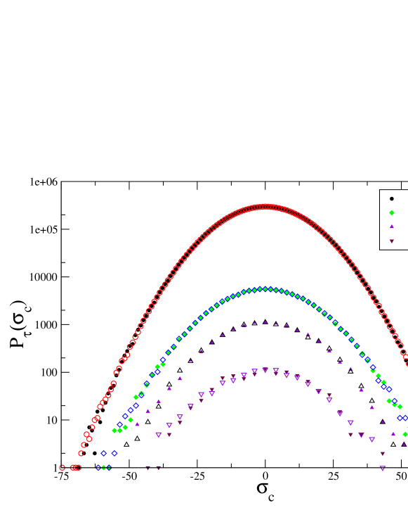
Figure 1: Probability distribution functions of $\sigma_{c}$ for different values of $\tau$ in equilibrium and for $\gamma=0.05$: for each value of $\tau$, filled symbols correspond to $\gamma=0$, open symbols to $\gamma=0.05$. On the $y$ axis the number of counts in each bin of the histogram is reported. A Gaussian distribution (non reported) perfectly describes all the curves in the range of fluctuations accessible to our simulation. The width of the distribution does not depend on $\tau$.

First, we study the PDF of $\dot{\sigma}_{c}(t)$ in the isokinetic ensemble. In Fig. 1 the function $P_{\tau}(\sigma_{c})$ is reported for different values of $\tau$ (from $0.2$ to $2000$) in equilibrium and for $\gamma=0.05$. The two sets of distributions are observed to coincide over the whole time range accessible to our simulations. Thus $P_{\tau}(\sigma_{c})$ is $\gamma$-independent and statement ii) is verified. At any time the distributions are well described by a Gaussian form

$$P_{\tau}(\sigma_{c})\propto\exp\left[-\frac{(\sigma_{c}-m_{c}(\tau))^{2}}{2S^{2}_{c}(\tau)}\right]$$ (10)

in the range of values of $\sigma_{c}$ accessible to our simulation. From the fit of the data reported in Fig. 1, we find that - within the statistical accuracy - the mean value of $\sigma_{c}$ is vanishing, as expected (see the discussion after Eq. 9). Moreover, recalling that

$$\sigma_{c}=\int_{0}^{\tau}\ dt\ \dot{\sigma}_{c}(t)=-\frac{1}{T}\int_{0}^{\tau}\ dt\frac{dV(q)}{dt}=\frac{V(0)-V(\tau)}{T}\ ,$$ (11)

we find

$$S^{2}_{c}(\tau)=\langle\sigma_{c}^{2}\rangle=2\frac{\langle V^{2}\rangle-\langle V(\tau)V(0)\rangle}{T^{2}}\sim 2\frac{\langle V^{2}\rangle-\langle V\rangle^{2}}{T^{2}}\ ,$$ (12)

where the last equality holds for large $\tau$. In our simulation $S_{c}^{2}(\tau)$ is observed to be $\tau$-independent and equal to $2(\langle V^{2}\rangle-\langle V\rangle^{2})/T^{2}$ (i.e. to the fluctuations of the potential energy) in the whole investigated $\tau$ range.

V Dissipative forces

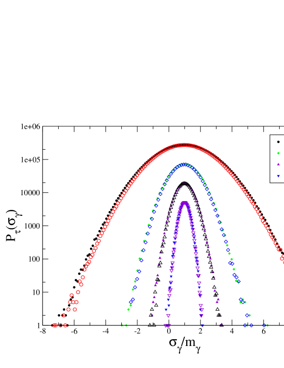
Figure 2: $P_{\tau}(\sigma_{\gamma})$ as a function of $\sigma_{\gamma}/m_{\gamma}$ at $T=0.5$ and $\gamma=0.05$: for each value of $\tau$ filled symbols correspond to the isokinetic ensemble, open symbols correspond to the isoenergetic ensemble. Ensemble equivalence holds for this quantity for any value of $\tau$. The distributions are Gaussian over the whole accessible range.

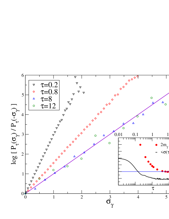
Figure 3: $\log P_{\tau}(\sigma_{\gamma})/P_{\tau}(-\sigma_{\gamma})$ as a function of $\sigma_{\gamma}$ for different values of $\tau$ in the isokinetic ensemble. The FT predicts the slope to be $1$ (continuous line) and is verified for $\tau\geq 8$. In the inset $2m_{\gamma}/S^{2}_{\gamma}$ (the slope of the lines) is reported as a function of $\tau$ together with the stress autocorrelation function (rescaled by an arbitrary factor).

We turn now to the analysis of the PDF of $\dot{\sigma}_{\gamma}(t)$, the entropy production due to the work of the dissipative forces. This quantity is reported in Fig. 2 for $T=0.5$ and $\gamma=0.05$ in both the isokinetic and isoenergetic ensemble. The PDFs in the two ensembles are found to coincide within the statistical uncertainties: thus, ensemble equivalence holds for the fluctuations of $\dot{\sigma}_{\gamma}$ at any $\tau$, proving the validity of statement iii).
In the isoenergetic ensemble, the distribution $P_{\tau}(\sigma_{\gamma})$ has been shown to verify the FR ECM , so we expect that the FR is also verified in the isokinetic ensemble for $\tau$ long enough. In Fig. 3 we report $\log P_{\tau}(\sigma_{\gamma})/P_{\tau}(-\sigma_{\gamma})$ as a function of $\sigma_{\gamma}$ calculated in the isokinetic ensemble. The FR predicts that the curve must be a straight line with slope $1$. From Fig. 3 we see that while for short $\tau$ values $\log P_{\tau}(\sigma_{\gamma})/P_{\tau}(-\sigma_{\gamma})$ appears to be linear but has a slope different from one, on increasing $\tau$ the slope tends toward one and the FR is indeed verified for $\tau\gtrsim 8$.
From Fig. 2 we can also observe that, similarly to that of $\dot{\sigma}_{c}(t)$, the PDF of $\dot{\sigma}_{\gamma}(t)$ is Gaussian over a very wide range. The same behavior has been observed and discussed in previous works BGG ; BCL ; GP . For a Gaussian distribution, $P_{\tau}(\sigma_{\gamma})\propto\exp\left[-\frac{(\sigma_{\gamma}-m_{\gamma}(\tau))^{2}}{2S^{2}_{\gamma}(\tau)}\right]$, the FR can be expressed as a relation between the mean value and the variance:

$$2m_{\gamma}=S^{2}_{\gamma}\ .$$ (13)

In the inset of Fig. 3 the quantity $2m_{\gamma}/S^{2}_{\gamma}$ is reported as a function of $\tau$. For $\tau\lesssim 20$ it coincides with the slope of $\log P_{\tau}(\sigma_{\gamma})/P_{\tau}(-\sigma_{\gamma})$ as a function of $\sigma_{\gamma}$ as derived from the main panel of Fig. 3. For $\tau\gtrsim 20$ in our simulation it is not possible to observe negative values of $\sigma_{\gamma}$ and the function $\log P_{\tau}(\sigma_{\gamma})/P_{\tau}(-\sigma_{\gamma})$ cannot be evaluated. However, the quantity $2m_{\gamma}/S^{2}_{\gamma}$ can be calculated also in absence of negative values of $\sigma_{\gamma}$ and is found to be equal to one within the statistical accuracy. In the inset of Fig. 3 the autocorrelation function of the entropy production $\langle\dot{\sigma}_{\gamma}(\tau)\dot{\sigma}_{\gamma}(0)\rangle$ is also reported as a function of $\tau$. This quantity, from Eq. (7), is proportional to the stress autocorrelation function $C(\tau)=\langle P_{yx}(\tau)P_{yx}(0)\rangle$. By defining the relaxation time of stress fluctuations $\tau_{\alpha}$ as $C(\tau_{\alpha})-C(\infty)=\frac{1}{2}[C(0)-C(\infty)]$, for the values of $\gamma$ and $T$ analyzed here we have $\tau_{\alpha}\sim 0.1$. From the inset of Fig. 3 we note that the FR is verified for $\tau\gtrsim 10^{2}\tau_{\alpha}$, which is statement iv).

VI Total phase space contraction rate

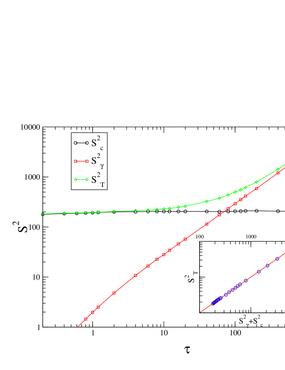
Figure 4: Variances of $\sigma_{c}$, $\sigma_{\gamma}$ and $\sigma_{T}$ as a function of $\tau$. In the inset, $S^{2}_{T}$ is reported as a function of $S^{2}_{c}+S^{2}_{\gamma}$; the data agree perfectly with the straight line of slope 1: then, $\sigma_{\gamma}$ and $\sigma_{c}$ are statistically independent. The fluctuations of $\sigma_{T}=\sigma_{\gamma}+\sigma_{c}$ are dominated at short times by $\sigma_{c}$ and at long times by $\sigma_{\gamma}$.

To conclude the analysis of the simulation data, we will now discuss the behavior of the fluctuations of the total phase space contraction rate, given by the sum of the two previously discussed contributions. Its PDF (not shown here) is also well described by a Gaussian distribution $P_{\tau}(\sigma_{T})\propto\exp\left[-\frac{(\sigma_{T}-m_{T}(\tau))^{2}}{2S^{2}_{T}(\tau)}\right]$ in the range of $\sigma_{T}$ accessible to our simulation. To relate the distribution of $\sigma_{T}$ to the ones of $\sigma_{c}$ and $\sigma_{\gamma}$, it is sufficient to discuss the behavior of the corresponding variances. In fact, remembering that $m_{c}=0$, $m_{\gamma}=m_{T}=1.39\tau$ and all the distributions are Gaussian in the observed range, the three distributions are fully specified by their variances. In Fig. 4 we report the variances $S^{2}_{c}$, $S^{2}_{\gamma}$ and $S^{2}_{T}$ as a function of $\tau$. In the inset, $S^{2}_{T}$ is reported as a function of $S^{2}_{c}+S^{2}_{\gamma}$ parametrically in $\tau$. From Fig. 4 we deduce that $\sigma_{c}$ and $\sigma_{\gamma}$ are statistically independent, as the variance of their sum is the sum of their variances, thus verifying statement i). Then, as $\sigma_{T}=\sigma_{c}+\sigma_{\gamma}$, its distribution is the convolution of the distributions of $\sigma_{c}$ and $\sigma_{\gamma}$. We observe also that $S^{2}_{c}$ is time-independent, while $S^{2}_{\gamma}=2m_{\gamma}=2.78\tau$ as predicted by the FR. Then, the fluctuations of the total entropy production are dominated by the conservative part at short times and by the dissipative part at long times. We have

$$\begin{cases}&P_{\tau}(\sigma_{T})\sim P_{\tau}(\sigma_{c})\hskip 28.45274pt\text{for small $\tau$ ($\lesssim 5$)}\\ &P_{\tau}(\sigma_{T})\sim P_{\tau}(\sigma_{\gamma})\hskip 28.45274pt\text{for large $\tau$ ($\gtrsim 1000$)}\end{cases}$$ (14)

This implies that the FR, being verified for $P_{\tau}(\sigma_{\gamma})$, is verified also for the PDF of the total entropy production $\sigma_{T}$, but for much longer times ($\tau\gtrsim 1000\sim 10^{4}\tau_{\alpha}$), and verifies statement v). Note that in our simulation it is not possible to directly check the validity of the FR in the asymptotic regime for $\sigma_{T}$ because it is not possible to observe negative values of $\sigma_{T}$ over so long times, so that the validity of the FR has to be deduced assuming a Gaussian form for the distribution $P_{\tau}(\sigma_{T})$ and checking that the ratio $2m_{T}/S^{2}_{T}$ is equal to one. However, by looking to the fluctuations of the dissipative part alone, the asymptotic regime is easily reached and a direct verification of the FR in the isokinetic ensemble is possible. Note also that the asymptotic regime for $\sigma_{T}$ corresponds to a regime in which the fluctuations due to the dissipative part are dominant and $\sigma_{T}\sim\sigma_{\gamma}$.

VII Fluctuation Relation for a Gaussian distribution

It is interesting to discuss briefly the implication of the FR if the distribution $P_{\tau}(\sigma)$ is Gaussian GAL ; BGG . In this case, the FR is equivalent to Eq. 13, and we can easily rewrite, using Eq. 7 and time-translation invariance:

$$\begin{split}&m_{\gamma}(\tau)=-\frac{\gamma}{T}\langle P_{yx}\rangle\tau\\ &S^{2}_{\gamma}(\tau)=\frac{\gamma^{2}}{T^{2}}\int_{0}^{\tau}dt\int_{0}^{\tau}dt^{\prime}\ \langle P_{yx}(t)P_{yx}(t^{\prime})\rangle=\frac{2\gamma^{2}\tau}{T^{2}}\int_{0}^{\tau}dt\ C(t)\end{split}$$ (15)

Then, Eq. 13 can be written in the following form

$$\langle P_{yx}\rangle=-\frac{\gamma}{T}\int_{0}^{\tau}dt\ C(t)$$ (16)

or, defining the viscosity $\eta=-\frac{\langle P_{yx}\rangle}{\gamma}$,

$$\eta=\frac{1}{T}\int_{0}^{\tau}dt\ C(t)$$ (17)

This (for $\tau\rightarrow\infty$) is an example of the well known Green-Kubo relation for the transport coefficients, that is strictly valid only in the $\gamma\rightarrow 0$ limit. Thus, if the distribution $P_{\tau}(\sigma_{\gamma})$ is a Gaussian, the FR implies the validity of the Green-Kubo relation for the viscosity also at finite $\gamma$.

VIII Conclusions

We discussed a simple model of a driven non-conservative system, i.e. a system in which the phase space volume is not conserved in equilibrium: a sheared liquid in the isokinetic ensemble.

We have shown that the total phase space contraction rate is the sum of two statistically independent contributions, defined in Eq. 9: the first, $\dot{\sigma}_{\gamma}$, is due to the work of the dissipative forces, and is the microscopic equivalent of the thermodynamic definition of entropy production given in Eq. 1. Its PDF is found to be the same in the two considered ensembles for any value of $\tau$, and verifies the FR in the large $\tau$ limit, $\tau\gtrsim 10^{2}\tau_{\alpha}$. The second contribution is $\gamma$-independent, has zero average and is negligible in the (very) large $\tau$ limit, $\tau\gtrsim 10^{4}\tau_{\alpha}$.

Then, we can conclude that:
a) The total entropy production can be identified, in the isokinetic ensemble, with the total phase space contraction rate $\dot{\sigma}_{T}$. The equivalence of isokinetic and isoenergetic ensembles holds, as conjectured in gal1 ; gal2 ; gal_stat ; gal_fluid . However, very large values of $\tau$, such that the contribution of $\dot{\sigma}_{c}$ can be neglected, have to be reached.
b) If one looks at that part of the phase space contraction rate that vanishes in the equilibrium limit, namely $\dot{\sigma}_{\gamma}$, equivalence holds for any $\tau$ and the FR is found to be verified at shorter times (by a factor $10^{2}$).
Obviously the first definition of entropy production rate has general validity gal2 , while the second one has to be discussed case by case by identifying the “relevant” part of the total phase space contraction rate. However, the second definition turns out to be very useful on a practical ground, because the very large $\tau$ values needed to observe the validity of the FR for the total phase space contraction rate are difficult to be reached in computer simulations. Also, this observation is relevant for experiments on real systems: indeed, equilibrium fluctuations of entropy production (analogous to $\dot{\sigma}_{c}$) are always present in real system in contact with a thermal bath, and it is impossible to separate the two contributions as in a numerical experiment. In planning experiments, one has then to check carefully that the time scales involved are such that the contribution analogous to $\dot{\sigma}_{c}$ is negligible.

It is a pleasure to thank Giovanni Gallavotti for a careful reading of the manuscript and for interesting suggestions and comments, and Alessandro Giuliani for useful discussions and encouragement.

References

- (1) G. Gallavotti, New methods in nonequilibrium gases and fluids, Proceedings of the conference Let’s face chaos through nonlinear dynamics, University of Maribor, ed. M. Robnik, Open Systems and Information Dynamics, Vol. 6, 1999; on-line at http://ipparco.roma1.infn.it.
- (2) G. Gallavotti, Nonequilibrium thermodynamics?, preprint cond-mat/0301172.
- (3) D.J. Evans and G.P. Morris, Statistical Mechanics of Nonequilibrium Liquids (Academic Press, London, 1990).
- (4) D. J. Evans, E. G. D. Cohen, and G. P. Morriss, Probability of second law violations in shearing steady states, Phys. Rev. Lett. 71, 2401 (1993).
- (5) G. Gallavotti and E.G.D. Cohen, Dynamical ensembles in nonequilibrium statistical mechanics, Phys. Rev. Lett. 74, 2694 (1995).
- (6) G. Gallavotti, Extension of Onsager’s reciprocity to large fields and the chaotic hypothesis, Phys. Rev. Lett. 77, 4334 (1996); G. Gallavotti, Chaotic hypothesis: Onsager reciprocity and fluctuation-dissipation theorem, J. Stat. Phys. 84, 899 (1996).
- (7) F. Bonetto, G. Gallavotti, and P. L. Garrido, Chaotic principle: an experimental test, Physica D 105, 226 (1997).
- (8) F. Bonetto, N. I. Chernov, J. L. Lebowitz, (Global and local) fluctuations of phase-space contraction in deterministic stationary non-equilibrium, Chaos 8, 823 (1998).
- (9) J. Kurchan, Fluctuation theorem for stochastic dynamics, J. Phys. A: Math. Gen. 31, 3719 (1998).
- (10) J. L. Lebowitz and H. Spohn, A Gallavotti-Cohen-type symmetry in the large deviation functional for stochastic dynamics, J. Stat. Phys. 95, 333 (1999).
- (11) L. Biferale, D. Pierotti, and A. Vulpiani, Time-reversible dynamical systems for turbulence, J. Phys. A: Math. Gen. 31, 21 (1998).
- (12) G. Gallavotti, F. Perroni, An experimental test of the local fluctuation theorem in chains of weakly interacting Anosov systems, preprint chao-dyn/9909007.
- (13) S. Ciliberto and C. Laroche, An experimental verification of the Gallavotti-Cohen fluctuation theorem, J. Phys. IV 8, 215 (1998).
- (14) W. I. Goldburg, Y. Y. Goldschmidt, and H. Kellay, Fluctuation and dissipation in liquid crystal electroconvection, Phys. Rev. Lett. 87, 245502 (2001).
- (15) K. Feitosa and N. Menon, A fluidized granular medium as an instance of the fluctuation theorem, preprint cond-mat/0308212.
- (16) G. Gallavotti, Statistical mechanics. A short treatise (Springer Verlag, Berlin, 2000).
- (17) G. Gallavotti, Foundation of fluid dynamics (Springer Verlag, Berlin, 2002).
- (18) M. P. Allen and D. J. Tildesley, Computer simulation of liquids (Oxford Science Publications, 1987).
- (19) G. Parisi, Off-equilibrium fluctuation dissipation relation in binary mixtures, Phys. Rev. Lett. 79, 3660 (1997).