Investigating Rare Events by Transition Interface Sampling

Daniele Moroni^a,∗, Titus S. van Erp^b, Peter G. Bolhuis^a

^aDepartment of Chemical Engineering, Universiteit van Amsterdam

Nieuwe Achtergracht 166, 1018 WV Amsterdam, The Netherlands

^bLaboratoire de Physique

Centre Européen de Calcul Atomique et Moléculaire,

Ecole Normale Supérieure de Lyon,

46 allée d’Italie, 69364 Lyon Cedex 07, France

Abstract

We briefly review simulation schemes for the investigation of rare transitions and we resume the recently introduced Transition Interface Sampling, a method in which the computation of rate constants is recast into the computation of fluxes through interfaces dividing the reactant and product state.

PACS: 82.20.Db, 82.20.Sb
keywords: Rare events; Rate constants; Transition Path Sampling.

^∗Corresponding author: Tel: +31-20-525-6917; fax: +31-20-525-5604;
email: moroni@science.uva.nl

1 Rare events

In many complex systems of physical importance transitions take place between stable states separated by a high (free) energy barrier. Examples are isomerizations in clusters, chemical reactions, protein folding and crystal nucleation. Molecular simulations techniques such as molecular dynamics (MD) in principle enable the computation of the reaction rate constants, the search for transition states and the exploration of reaction mechanisms. But since the rate constant of the transition depends exponentially on the activation barrier height, the expectation time of a transition can easily become orders of magnitude longer than the molecular timescale which is usually measured in femtoseconds. Hence, when using straightforward MD the study of these rare events is far beyond current computer capabilities.

In the past decade, a number of methods has been proposed that aim to tackle this timescale problem from different points of view. One class of methods focusses on escaping the initial state without making assumptions on the final state. This can be achieved by, for instance, artificially increasing the frequency of the rare event in a controlled way. The methods of Voter and collaborators follow this approach: hyperdynamics [1, 2] aims at lowering the energy difference between the top of the barrier and the initial basin, the parallel replica method [3] exploits the power of parallel processing to extend the molecular simulation time, and temperature-accelerated dynamics [4, 5] speeds up the event by raising the temperature. The idea of driving energy into the system to escape the basin of the energy minimum in which the system is initially prepared is also at the basis of conformational flooding [6], the Laio-Parrinello method [7, 8], and the enhanced sampling of a given reaction coordinate [9]. Another possible route is to coarse-grain the molecular dynamics on the fly and explore the resulting free-energy landscape [10]. Several methods are devoted to the exploration of the full potential energy surface through all its minima and saddle points. Examples are eigenvector following [11, 12], the activation-relaxation technique of Barkema and Mousseau, [13], the dimer method of Henkelmann and Jónsson [14], the kinetic Monte Carlo (MC) approach [15, 16, 17], and the discrete path sampling of Wales [18, 19].

When the initial and final state are known it is possible to generate paths connecting the two in the form of a discretized chain of states. This is the basis of a second class, the so-called two point boundary methods. One option is to find a minimal energy path on the potential energy surface, as in the Nudged Elastic Band method of Jónsson and collaborators [20, 21, 22, 23] and in the string method of E et al. [24], or to find a true dynamical path by minimizing a suitably chosen action [25]. Another possibility is to use modified stochastic equations of motion that guide the system from the initial to the final state [26].

To summarize, one can say that each of the above methods is well suited in one specific subclass of systems, but they also have their specific drawbacks. Some are inefficient for high dimensional systems or only give structural information and neglect the dynamics. Others are designed to find only one transition or make heavily use on assumptions or prior knowledge of the system. In complex systems at finite temperature, concepts like the minimum energy (or action) path or the lowest saddle point are not very useful. The reaction is rather described by a ensemble of paths. Similarly, one cannot speak of a particular transition state but only of an ensemble of transition states.

An important quantity describing the kinetics of rare events is the rate constant. The traditional way to calculate rate constants in complex condensed matter system is by the reactive flux method based on Transition State Theory [27, 28, 29, 30, 31]. This method consists of two stages. First, the free energy is computed as a function of selected degrees of freedom describing the reaction from the initial to the final state (the reaction coordinate), for instance by biased sampling techniques [32, 33, 34]. This step is complemented with the calculation of a dynamical transmission coefficient, by starting short trajectories from the maximum of the free energy barrier. However, in complex systems the correct reaction coordinate can be exceedingly difficult to find. If the reaction coordinate does not capture the molecular mechanism, the biased sampling methods will suffer from substantial hysteresis when following the system over the barrier. Moreover, even if the free energy profile is obtained correctly for this particular (but wrong) reaction coordinate, the corresponding transmission coefficient will be very low, making an accurate evaluation problematic.

To overcome these problems, Chandler and collaborators developed the Transition Path Sampling (TPS) method. This technique gathers a collection of true dynamical trajectories connecting the states without any a priori assumption of the reaction coordinate. From the ensemble of pathways rate constants can be calculated and reaction mechanisms can be extracted [35, 36, 37, 38]. The method can be combined with parallel tempering [39] and stochastic dynamics can be used for the case of diffusive barriers [40, 41]. Successful applications of TPS are, among others, ion pair dissociation in water [42, 43], alanine dipeptide in vacuum and in aqueous solution [44], neutral [45] and protonated [46, 47] water clusters, autoionization in water [48], and the folding of a polypeptide [49]. For a detailed review on TPS see Refs. [50, 51, 52]. Similar techniques by Elber and Olender [53, 54, 55] and Doniach et al [56] sample discretized stochastic pathways based on the Onsager-Machlup action. Finally, we mention the topological method of Tănase-Nicola and Kurchan [57] in which they suggest to use TPS in combination with saddle point searching vector walkers.

In this paper we focus on transition path sampling, and in particular on the Transition Interface Sampling (TIS) method, a recent improvement over the TPS rate constant calculation [58]. We briefly review the TIS method and give an example of its application. Further details on the derivations, algorithms and applications can be found in Ref. [58].

2 Transition Interface Sampling

Consider a dynamical system prepared in the initial state $A$. The state is stable in the sense that trajectories will stay in that state for a time long compared to the molecular time scale (e.g. vibrations). Eventually, the trajectories cross the barrier and reach the final state $B$. If the barrier is sufficiently high the system shows exponential relaxation and the rate constant $k_{AB}$ is well defined. In what follows we assume that we can compute the evolution of trajectories in phase space, without further specifying the details of the dynamics. For instance, we could use deterministic integration of Hamilton’s equations of motion or stochastic dynamics generated by a Langevin equation.

The starting point of TIS is the partitioning of phase space by interfaces. We define an order parameter $\lambda(x)$ as a function of the phase space point $x$ (consisting of positions and momenta of all particles in the system) and the interfaces $i=0\ldots n$ as the hypersurfaces $\{x|\lambda(x)=\lambda_{i}\}$. We assume that the interfaces do not intersect, that $\lambda_{i-1}<\lambda_{i}$, and we describe the boundaries of state $A$ and $B$ by $\lambda_{0}$ and $\lambda_{n}$ respectively. In the same spirit of TPS, the TIS method has the non-trivial advantage that the order parameter $\lambda(x)$ does not have to be a properly chosen reaction coordinate capturing the essence of the dynamical mechanism. Instead, it is sufficient that this function is able to characterize the basins of attraction of the stable states [50]. The basis of the TIS method is the microscopic equation for the rate constant

$$k_{AB}=\langle\phi_{n,0}\rangle/\langle h_{\mathcal{A}}\rangle.$$ (1)

Here $\langle\phi_{i,0}\rangle$ is the effective positive flux from interface 0 – i.e. from state $A$ – through interface $i$, where effective means that recrossings are not being counted. Equivalently, it is an average over all phase points that are first crossings through interface $i$ but belong to trajectories that originated in $A$. The denominator $\langle h_{\mathcal{A}}\rangle$ is a normalization factor taking into account all the phase points for which the corresponding trajectories come directly from $A$ without having visited $B$ (naturally, this includes the entire region A, and most part of the basin of attraction of A). In a simulation the ratio in Eq. (1) is computed by starting a MD simulation in state $A$ and counting the number of effective crosses with interface $n$, i.e. the number of times it reaches state $B$, per time unit. Since the transitions are rare, Eq. (1) is of no practical use in this form, because the simulation would have to be long enough to see at least one spontaneous event. We can improve efficiency by relating the effective flux $\langle\phi_{i,0}\rangle$ through an interface $i$ to the effective flux $\langle\phi_{i-1,0}\rangle$ through an interface $i-1$ closer to $A$:

$$\langle\phi_{i,0}\rangle=\langle\phi_{i-1,0}\rangle\cdot P_{A}(\lambda_{i}|\lambda_{i-1}).$$ (2)

Here, $P_{A}(\lambda_{i}|\lambda_{j})$ is the conditional probability that a trajectory coming from $A$ crosses interface $i$ provided that it has passed interface $j$. Iteratively substituting Eq. (2) in Eq. (1) we can write

$$k_{AB}=\frac{\langle\phi_{1,0}\rangle}{\langle h_{\mathcal{A}}\rangle}\prod_{i=1}^{n-1}P_{A}(\lambda_{i+1}|\lambda_{i})\equiv\frac{\langle\phi_{1,0}\rangle}{\langle h_{\mathcal{A}}\rangle}P_{A}(\lambda_{n}|\lambda_{1}),$$ (3)

which is the key equation of TIS. Similar equations can be written for the backward rate constant $k_{BA}$.

We compute the first term in Eq. (3) by starting a simulation in $A$ and counting the number of crossings with interface 1 per unit time. A statistically accurate value can be obtained by choosing the interface close enough to the initial state. The second term $P_{A}(\lambda_{n}|\lambda_{1})$ is computed using the factorization in Eq. (3). First, we generate an ensemble of paths that start in $A$, cross interface 1 and eventually return to $A$ or, alternatively, continue to cross the next interface 2. The probability $P_{A}(\lambda_{2}|\lambda_{1})$ is the ratio of the number of paths that reach interface 2 to the total number of sampled paths. Subsequently, we generate an ensemble of paths starting in $A$ and crossing interface 2, from which the next term $P_{A}(\lambda_{3}|\lambda_{2})$ can be obtained, and so on until we reach interface $n$ and thus state $B$. Each step consists of a sampling of paths starting in $A$ and crossing interface $i=1\ldots n-1$. This procedure is similar in spirit to the umbrella sampling technique in which different windows are employed to obtain free energy profiles [27]. Note that the final rate constant $k_{AB}$ is independent of the choice of the interfaces as long as the first and last one are inside the basin of attraction of the stable states $A$ and $B$ respectively.

The path ensembles are generated by constructing a random walk in path space employing a MC algorithm. Fundamental for both the TPS and TIS methods is the MC move that generates a new path from an existing one, the shooting move [36]. An existing path between the initial and final state is stored as collection of discrete time-slices. In a shooting move, a time slice is chosen at random, the momenta of all particles are slightly changed, and a new trajectory is created by integrating the system forward and backward in time. The new path is accepted with a probability chosen such that detailed balance is obeyed. In contrast to TPS, the path length does not have a prefixed value [36], but is allowed to vary because the integration of the equations of motion is stopped when one of the two interfaces of the corresponding ensemble is reached [58].

3 Discussion

We tested the TIS method on the isomerization of a diatomic molecule immersed in a repulsive fluid, a simple model system used before to test the TPS algorithms [38]. We report some details and the results in Fig. 1; more details can be found in Ref [58]. The forward rate constant for the isomerization corresponds to an average transition time $k_{AB}^{-1}=(3.6\pm 0.1)s$ in real units for argon, which is indeed many orders of magnitude beyond the MD time-step $\sim 4fs$. In Ref. [58] we showed that TIS is at least a factor 2 more efficient than TPS when computing the rate constant at equivalent conditions and same final relative error. The efficiency increases to 5 or more in systems with many recrossings.

The TIS algorithm makes use of the MC moves developed for TPS, and in this sense TIS can be considered an extension of TPS. TIS retains the good features, such as the independence of prior knowledge of a reaction coordinate [50], and improves on the weaker points, for example, minimizing computational effort by allowing a variable path length. The spirit behind the TIS methodology for computing rate constants, however, is different. The concept of a positive effective flux gives a faster convergence because only positive terms contribute to the rate. The implementation of the computer algorithm becomes easier and one can apply multidimensional or discrete interface order parameters. These advantages make TIS more efficient in terms of computational effort. Finally, in some cases a better characterization of true reactive paths can be achieved and non-true recrossings can be avoided through a proper choice of the interfaces, for instance, imposing kinetic energy constraints [58].

The TIS method has been successfully applied to two realistic cases, the folding of a polypeptide [49] and hydration of ethylene [59]. In this last case the method was combined with quantum ab-initio MD simulations. A recent variation of the TIS method for diffusive systems exploits very efficiently the loss of long time scale correlation by using a recursive reformulation of the crossing probability and the sampling of much shorter paths [60]. These results show that TIS is capable of studying rare event processes in complex systems efficiently and encourage even more challenging applications, such as isomerization in clusters and crystal nucleation, on which we plan to report in the future.

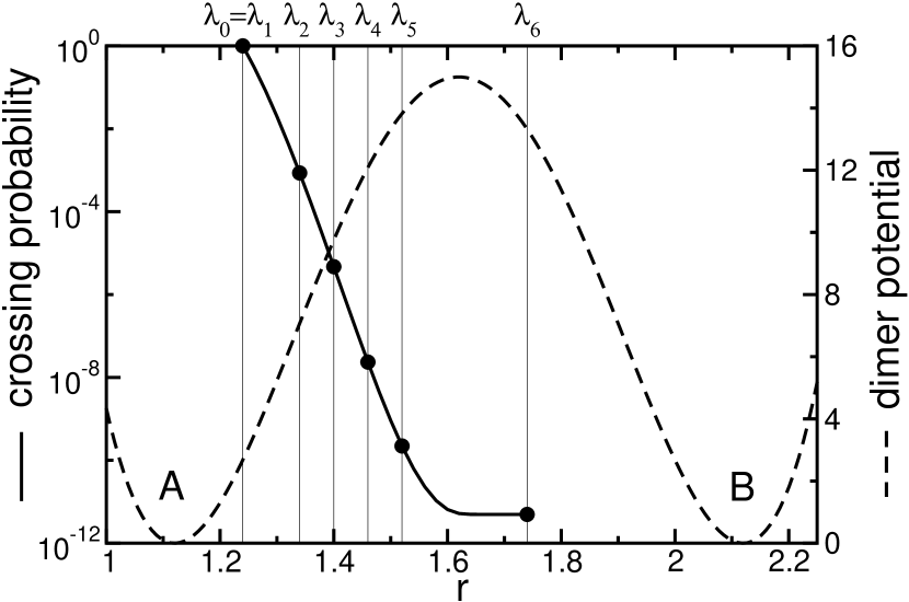
Figure 1: The dimer inter-particle potential (dashed line) and the TIS crossing probability $P_{A}(\lambda,\lambda_{1})$ (solid line) as function of the order parameter $\lambda=r$, the dimer inter-particle separation. State $A$ at the first minimum of the double-well corresponds to a compact state of the molecule and state $B$ at second minimum to an extended state. The number of 2D solvent particles with unit diameter is 25, the density is 0.7, the total energy was fixed at E=25 (all in Lennard-Jones reduced units [27]). We computed the flux $\langle\phi_{1,0}\rangle/\langle h_{\mathcal{A}}\rangle=0.1196\pm 0.0005$, and the crossing probability function $P_{A}(\lambda|\lambda_{1})$ by matching the partial functions $P_{A}(\lambda_{i+1}|\lambda_{i})$, $i=1\ldots 5$ in five windows of path ensemble simulations.The interfaces in between are indicated by vertical lines. The error on the data points is within symbol size. The smooth line joining the points was created using a finer grid of interfaces [58]. The horizontal plateau when approaching state $B$ at $\lambda_{n=6}=1.74$ is an expression of the commitment of the trajectories to the final stable state. Paths that cross $r\simeq 1.7$ always reach eventually the final interface without going back to $A$. The value of the plateau equals $P_{A}(\lambda_{n},\lambda_{1})$.

References

- [1] A. F. Voter, J. Chem. Phys. 106, 4665 (1997).
- [2] A. F. Voter, Phys. Rev. Lett. 78, 3908 (1997).
- [3] A. F. Voter, Phys. Rev. B 57, R13985 (1998).
- [4] A. F. Voter and M. R. Sørensen, Mat. Res. Soc. Symp. Proc. 538, 427 (1999).
- [5] M. R. Sørensen and A. F. Voter, J. Chem. Phys. 112, 9599 (2000).
- [6] H. Grubmüller, Phys. Rev. E 52, 2893 (1995).
- [7] A. Laio and M. Parrinello, Proc. Natl. Acad. Sci. USA 99, 12562 (2002).
- [8] M. Iannuzzi, A. Laio, and M. Parrinello, Phys. Rev. Lett. 90, 238302 (2003).
- [9] S. Melchionna, Phys. Rev. E 62, 8762 (2000).
- [10] G. Hummer and I. G. Kevrekidis, J. Chem. Phys. 118, 10762 (2003).
- [11] C. J. Cerjan and W. H. Miller, J. Chem. Phys. 75, 2800 (1981).
- [12] J. P. K. Doye and D. J. Wales, Z. Phys. D 40, 194 (1997).
- [13] G. T. Barkema and N. Mousseau, Phys. Rev. Lett. 77, 4358 (1996).
- [14] G. Henkelmann and H. Jónsson, J. Chem. Phys. 111, 7010 (1999).
- [15] D. T. Gillespie, J. Comput. Phys. 28, 395 (1978).
- [16] A. F. Voter, Phys. Rev. B 34, 6819 (1986).
- [17] K. A. Fichthorn and W. H. Weinberg, J. Chem. Phys. 95, 1090 (1991).
- [18] D. J. Wales, Mol. Phys. 100, 3285 (2002).
- [19] D. J. Wales, Energy Landscapes (Cambridge University Press, 2003).
- [20] G. Mills, H. Jónsson, and G. K. Schenter, Surf. Sci. 324, 305 (1995).
- [21] G. Henkelman, B. P. Uberuaga, and H. Jónsson, J. Chem. Phys. 113, 9901 (2000).
- [22] G. Henkelman and H. Jónsson, J. Chem. Phys. 113, 9978 (2000).
- [23] H. Jónsson, G. Mills, and K. W. Jacobsen, in Classical and Quantum Dynamics in Condensed Phase Simulations, edited by B. J. Berne, G. Ciccotti, and D. Coker (World Scientific, Singapore, 1998).
- [24] W. E, W. Ren, and E. Vanden-Eijnden, Phys. Rev. B 66, 052301 (2002).
- [25] D. Passerone and M. Parrinello, Phys. Rev. Lett. 87, 108302 (2001).
- [26] D. M. Zuckerman and T. B. Woolf, J. Chem. Phys. 11, 9475 (1999).
- [27] D. Frenkel and B. Smit, Understanding molecular simulation, 2nd ed. (Academic Press, San Diego, CA, 2002).
- [28] J. C. Keck, Adv. Chem. Phys. 13, 85 (1967).
- [29] J. B. Anderson, J. Chem. Phys. 58, 4684 (1973).
- [30] C. H. Bennett, in Algorithms for Chemical Computations, ACS Symposium Series No. 46, edited by R. Christofferson (American Chemical Society, Washington, D.C., 1977).
- [31] D. Chandler, J. Chem. Phys. 68, 2959 (1978).
- [32] G. M. Torrie and J. P. Valleau, Chem. Phys. Lett. 28, 578 (1974).
- [33] E. A. Carter, G. Ciccotti, J. T. Hynes, and R. Kapral, Chem. Phys. Lett. 156, 472 (1989).
- [34] G. Ciccotti, in Computer Simulations in Materials Science, edited by M. Meyer and V. Pontikis (Kluwer, Dordrecht, 1991), pp. 365–396.
- [35] C. Dellago, P. G. Bolhuis, F. S. Csajka, and D. Chandler, J. Chem. Phys. 108, 1964 (1998).
- [36] C. Dellago, P. G. Bolhuis, and D. Chandler, J. Chem. Phys. 108, 9236 (1998).
- [37] P. G. Bolhuis, C. Dellago, and D. Chandler, Faraday Discuss. 110, 421 (1998).
- [38] C. Dellago, P. G. Bolhuis, and D. Chandler, J. Chem. Phys. 110, 6617 (1999).
- [39] T. J. H. Vlugt and B. Smit, Phys. Chem. Comm. 2, 1 (2001).
- [40] P. G. Bolhuis, J. Phys. Cond. Matter 15, S113 (2003).
- [41] G. E. Crooks and D. Chandler, Phys. Rev. E 64, 026109 (2001).
- [42] P. L. Geissler, C. Dellago, and D. Chandler, J. Phys. Chem. B 103, 3706 (1999).
- [43] J. Martí, F. S. Csajka, and D. Chandler, Chem. Phys. Lett. 328, 169 (2000).
- [44] P. G. Bolhuis, C. Dellago, and D. Chandler, Proc. Natl. Acad. Sci. USA 97, 5877 (2000).
- [45] J. Rodriguez, G. Moriena, and D. Laria, Chem. Phys. Lett. 356, 147 (2002).
- [46] P. L. Geissler, C. Dellago, and D. Chandler, Phys. Chem. Chem. Phys. 1, 1317 (1999).
- [47] D. Laria, J. Rodriguez, C. Dellago, and D. Chandler, J. Phys. Chem. A 105, 2646 (2001).
- [48] P. L. Geissler et al., Science 291, 2121 (2001).
- [49] P. G. Bolhuis, Proc. Nat. Acad. Sci. USA 100, 12129 (2003).
- [50] P. G. Bolhuis, D. Chandler, C. Dellago, and P. L. Geissler, Annu. Rev. Phys. Chem. 53, 291 (2002).
- [51] C. Dellago, P. G. Bolhuis, and P. L. Geissler, Adv. Chem. Phys. 123, 1 (2002).
- [52] P. G. Bolhuis, C. Dellago, P. L. Geissler, and D. Chandler, J. Phys. Cond. Matter 12, A147 (2000).
- [53] R. Olender and R. Elber, J. Chem. Phys. 105, 9299 (1996).
- [54] V. Zaloj and R. Elber, Comp. Phys. Comm. 128, 118 (2000).
- [55] R. Elber, J. Meller, and R. Olender, J. Phys. Chem. B 103, 899 (1999).
- [56] P. Eastman, N. Grønbech-Jensen, and S. Doniach, J. Chem. Phys. 114, 3823 (2001).
- [57] S. Tănase-Nicola and J. Kurchan, Phys. Rev. Lett. 91, 188302 (2003).
- [58] T. S. van Erp, D. Moroni, and P. G. Bolhuis, J. Chem. Phys. 118, 7762 (2003).
- [59] T. S. van Erp, Ph.D. thesis, Universiteit van Amsterdam, 2003.
- [60] D. Moroni, P. G. Bolhuis, and T. S. van Erp, submitted, cond-mat/0310466 (2003).