Renormalization group study of the conductances of interacting quantum wire systems with different geometries

Abstract

We examine the effect of interactions between the electrons on the Landauer-Büttiker conductances of some systems of quantum wires with different geometries. The systems include a long wire with a stub in the middle, a long wire containing a ring which can enclose a magnetic flux, and a system of four long wires which are connected in the middle through a fifth wire. Each of the wires is taken to be a weakly interacting Tomonaga-Luttinger liquid, and scattering matrices are introduced at all the junctions present in the systems. Using a renormalization group method developed recently for studying the flow of scattering matrices for interacting systems in one dimension, we compute the conductances of these systems as functions of the temperature and the wire lengths. We present results for all three regimes of interest, namely, high, intermediate and low temperature. These correspond respectively to the thermal coherence length being smaller than, comparable to and larger than the smallest wire length in the different systems, i.e., the length of the stub or each arm of the ring or the fifth wire. The renormalization group procedure and the formulae used to compute the conductances are different in the three regimes. In particular, the dimensionality of the scattering matrix effectively changes when the thermal length becomes larger than the smallest wire length. We also present a phenomenologically motivated formalism for studying the conductances in the intermediate regime where there is only partial coherence. At low temperatures, we study the line shapes of the conductances versus the energy of the electrons near some of the resonances; the widths of the resonances are found to go to zero with decreasing temperature. Our results show that the Landauer-Büttiker conductances of various systems of experimental interest depend on the temperature and lengths in a non-trivial way when interactions are taken into account.

]

I Introduction

The increasing sophistication in the fabrication of semiconductor heterostructures and carbon nanotubes in recent years have made it possible to study electronic transport in different geometries. For instance, three-arm and four-arm quantum wire systems have been fabricated by voltage-gate patterning on the two-dimensional electron gas in GaAs heterojunctions [1, 2]. Other systems of interest include Y-branched carbon nanotubes [3], crossed carbon nanotubes [4], mesoscopic rings [5, 6], and quantum wire systems with stubs [7]. There have also been many theoretical studies of transport in systems with various geometries [8, 9, 10, 11, 12].

Studies of ballistic transport in a quantum wire (QW) have led to a clear understanding of the important role played by both scattering of the electrons and the interactions between the electrons inside the QW [13, 14, 15, 16]. The scattering can occur either due to impurities inside the QW or at the contacts lying between the QW and its reservoirs. A theoretical analysis using bosonization [17] and the renormalization group (RG) method typically shows that repulsive interactions between electrons tend to increase the effective strength of the back-scattering as one goes to longer length scales; experimentally, this leads to a power-law decrease in the conductance as the temperature is reduced or the wire length is increased [18]. Motivated by this understanding of the effects of interaction on scattering, there have been several studies of the interplay between the effects of interactions on one hand, and either a single junction between three of more QWs [19, 20, 21, 22], or more complicated geometries [23, 24, 25, 26] on the other. Using a RG technique introduced in Ref. [27], the effects of a junction (which is characterized by an arbitrary scattering matrix $S$) has been studied in some detail [21]. It is now natural to extend these studies to systems of QWs which are of experimental interest and which can have with more complicated geometries involving more than one junction.

In this paper, we will study the effect of interactions on the Landauer-Büttiker conductances of three systems of quantum wires with different geometries. These systems are shown in Figs. 1-3, and we will refer to them as the stub, the ring and the four-wire system respectively. The stub system consists of two long wires, labeled as 1 and 3, with a stub labeled as 2 being attached to the junction of 1 and 3. The ring consists of two long wires, labeled as 1 and 3, between which there is a ring which can possibly enclose a magnetic flux; the two arms of the ring, labeled as 2 and 4, will be assumed to have the same length for convenience. The four-wire system consists of four long wires labeled as 1, 2, 3 and 4. The junction of 1 and 2 is connected to the junction of 3 and 4 by a fifth wire labeled as 5. The length of wire 2 in the stub system, the length of each of the arms 2 and 4 in the ring system, and the length of wire 5 in the four-wire system will all be denoted by $L_{S}$. Each of the junctions present in the different systems is governed by a $3\times 3$ scattering matrix $S$ which is unitary. We will assume that each of the wires in the various systems can be described as a one-channel weakly interacting Tomonaga-Luttinger liquid (TLL). For simplicity, we will ignore the spin of the electrons in this paper.

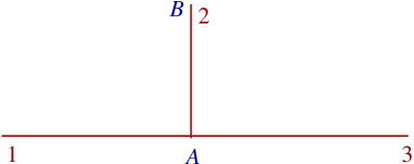
FIG. 1.: The stub system, showing two long wires labeled as 1 and 3, and a stub labeled as 2. The lower end of the stub where three wires meet and the upper end of the stub are denoted by $A$ and $B$ respectively.

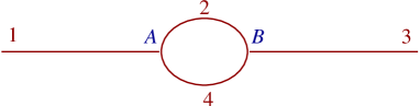
FIG. 2.: The ring system, showing two long wires labeled as 1 and 3, the two arms of the ring labeled as 2 and 4, and two three-wire junctions labeled as $A$ and $B$.

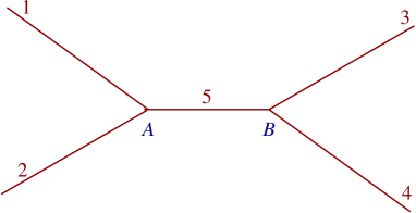
FIG. 3.: The four-wire system, showing four long wires labeled as 1, 2, 3 and 4, a connecting wire in the middle labeled as 5, and two three-wire junctions labeled as $A$ and $B$.

In Sec. II, we will first summarize the RG method developed in Ref. [21] for studying the flow of the $S$-matrix at a junction due to the interactions in the different wires connected to that junction. We will then describe our method for carrying out the RG analysis of the $S$-matrices at the various junctions of the different systems. In Sec. III, we will describe the procedure for computing the transmission probabilities (and conductances) of a system given the form of the $S$-matrices at all its junctions. It turns out that both the RG procedure and the route from the $S$-matrix to the conductances depend on the range of temperatures that one is considering. There is a length scale, called the thermal coherence length $L_{T}$, which governs the typical distance beyond which the phase of the electron wave function becomes uncorrelated with its initial phase. The regimes of high, intermediate and low temperatures are governed respectively by the condition that $L_{T}$ is much smaller than, comparable to or much larger than the length scale $L_{S}$ defined above for the three systems; correspondingly, we have complete incoherence, partial coherence and complete coherence for the phase. The intermediate temperature range is the most difficult one to study, both for using the RG method and for computing the conductances. Based on some earlier ideas [28, 29], we will describe a phenomenological way of introducing partial coherence which will lead to expressions for the transmission probabilities which interpolate smoothly between the coherent and incoherent expressions.

In Secs. IV-VI, we will apply the formalism outlined in the previous sections to the stub, ring and four-wire systems respectively. In each case, the transmission probabilities at intermediate and low temperatures (i.e., the partially and completely coherent regimes) will be found to depend sensitively on the phase $\eta=e^{i2k_{F}L_{S}}$; here $k_{F}$ is the wave number of the electrons which are assumed to come into or leave the QW system with a momentum which is equal to the Fermi momentum in the reservoirs. In particular, certain values of $\eta$ can lead to resonances and anti-resonances i.e., maxima and minima in the transmission probabilities. In the ring system, there is another important phase which governs the possibility of resonance, namely, $e^{ie\phi_{B}/\hbar c}$, where $\phi_{B}$ is the magnetic flux enclosed by the ring, and $e$ and $c$ are the electron charge and the speed of light respectively. In each system, we will see how the conductances vary with the temperature in a non-trivial way as a result of the interactions. This is the main point of our paper, namely, that interactions between the electrons lead to certain power-laws in the temperature and length dependences of the conductances of experimentally realizable quantum wire systems.

II Renormalization Group Method for Systems with Junctions

In this section, we will first present the RG procedure developed in Ref. [21] for studying how the effect of a single junction varies with the length scale. We will then describe how the RG method has to be modified when a system has more than one junction.

A junction is a point where $N$ semi-infinite wires meet. Let us denote the various wires by a label $i$, where $i=1,2,\cdots,N$. As we approach the junction, the incoming and outgoing one-electron wave functions on wire $i$ approach values which are denoted by $\psi_{Ii}$ and $\psi_{Oi}$ respectively; we can write these more simply as two $N$-dimensional columns $\psi_{I}$ and $\psi_{O}$. The outgoing wave functions are related to the incoming ones by a $N\times N$ scattering matrix,

$$\psi_{O}~{}=~{}S~{}\psi_{I}~{}.$$ (1)

Current conservation at the junction implies that $S$ must be unitary. (If we want the junction to be invariant under time reversal, $S$ must also be symmetric). The diagonal entries of $S$ are the reflection amplitudes $r_{ii}$, while the off-diagonal entries are the transmission amplitudes $t_{ij}$ to go from wire $j$ to wire $i$. We will assume that the entries of $S$ do not have any strong dependence on the energy of the electrons.

Let us now consider a simple model for interactions between the electrons, namely, a short-range density-density interaction of the form

$$H_{\rm int}~{}=~{}\frac{1}{2}~{}\int\int dxdy~{}\rho(x)~{}V(x-y)~{}\rho(y)~{},$$ (2)

where $V(x)$ is a real function of $x$, and the density $\rho(x)$ is given in terms of the second-quantized fermion field $\Psi(x)$ as $\rho=\Psi^{\dagger}\Psi$. [The assumption of a short-ranged interaction is often made in the context of the TLL description of systems of interacting fermions in one dimension.] We define a parameter $g_{2}$ which is related to the Fourier transform of $V(x)$ as $g_{2}={\tilde{V}}(0)-{\tilde{V}}(2k_{F})$. Different wires may have different values of this parameter which we will denote by $g_{2i}$. For later use, we define the dimensionless constants

$$\alpha_{i}~{}=~{}\frac{g_{2i}}{2\pi\hbar v_{F}}~{},$$ (3)

where we assume that the velocity

$$v_{F}~{}=~{}\frac{\hbar k_{F}}{m}$$ (4)

is the same on all wires. In this work, we will be interested in the case in which the interactions are weak and repulsive, i.e., the parameters $\alpha_{i}$ are all positive and small.

We are now ready to present the RG equation for the matrix $S$ which was derived in Ref. [21]. It will be useful to briefly discuss the derivation of the RG equation. A reflection from a junction, denoted by the amplitude $r_{ii}$ in wire $i$, leads to Friedel oscillations in the electron density in that wire. If $x$ denotes the distance of a point from the junction, the form of the oscillation at that point is given by the imaginary part of $r_{ii}e^{i2k_{F}x}/(2\pi x)$. As a result of the interactions, an electron traveling in that wire gets reflected from these oscillations. The amplitude of the reflection from the oscillations is proportional to $\alpha_{i}r_{ii}/2$ if the electron is reflected away from the junction, and to $\alpha_{i}r_{ii}^{*}/2$ if the electron is reflected towards the junction. These reflections renormalize the bare $S$-matrix which characterizes the junction at the microscopic length scale. The entries of $S$ therefore become functions of the length scale $L$; we define the logarithm of the length scale as $l={\rm ln}(L/d)$, where $d$ is a short-distance cutoff such as the average interparticle spacing. It is convenient to define a $N\times N$ diagonal matrix $M$ whose entries are given by

$$M_{ii}~{}=~{}\frac{1}{2}~{}\alpha_{i}r_{ii}~{}.$$ (5)

Then the RG equation for $S$ is found to be [21]

$$\frac{dS}{dl}~{}=~{}M~{}-~{}SM^{\dagger}S$$ (6)

to first order in the $\alpha_{i}$. (This equation is therefore perturbative in the interaction strength). One can verify from Eq. (6) that $S$ remains unitary under the RG flow; it also remains symmetric if it begins with a symmetric form. The fixed points of Eq. (6) are given by the condition $SM^{\dagger}=MS^{\dagger}$, i.e., $SM^{\dagger}$ must be Hermitian.

We can study the linear stability of a fixed point by deviating slightly from it, and seeing how the deviation grows to first order under the RG flow. Let us denote a fixed point by the matrix $S_{0}$ and a deviation by $\epsilon S_{1}$, where $\epsilon$ is a small real parameter and $S_{1}$ is a matrix; we require that the matrix $S=S_{0}+\epsilon S_{1}$ is unitary up to order $\epsilon$. (We can think of $S_{1}$ as defining the “direction” of the deviation). We substitute $S$ in Eq. (6) and then demand that $S_{1}$ should take such a form that the RG equation reduces to

$$\frac{d\epsilon}{dl}~{}=~{}\mu\epsilon~{},$$ (7)

where $\mu$ is a real number. We then call the direction $S_{1}$ stable, unstable and marginal (to first order) if $\mu<0,>0$ and $0$ respectively. All fixed points have at least one exactly marginal direction which corresponds to multiplying the matrix $S_{0}$ by a phase; clearly this leaves Eq. (6) invariant.

In this paper, we will be concerned with the RG flow of $S$-matrices which are 2, 3 and 4 dimensional. For convenience, we will assume certain symmetries in each of these cases. It is useful to discuss these symmetries here, and how they lead to some simplifications for the RG flows.

We first consider a two-wire system in which there is complete symmetry between the wires which we will label as 1 and 3. Namely, the interaction parameters are equal, $\alpha_{1}=\alpha_{3}=\alpha$, and the scattering matrix has the form

$$S_{2D}~{}=~{}\left(\begin{array}[]{cc}a&b\\ b&a\end{array}\right)~{}.$$ (10)

Unitarity implies that we can parametrize $a$ and $b$ as

$$a = -~{}\frac{i\lambda e^{i\theta}}{1~{}+~{}i\lambda}~{},$$ (11)

$$b = \frac{e^{i\theta}}{1~{}+~{}i\lambda}~{},$$ (12)

where $\lambda$ and $\theta$ are real. Eq. (6) then leads to the following differential equations

$$\frac{d\lambda}{dl} = \alpha~{}\lambda~{},$$ (13)

$$\frac{d\theta}{dl} = \frac{\alpha\lambda}{1~{}+~{}\lambda^{2}}~{}.$$ (14)

The reflection and transmission probabilities $|a|^{2}$ and $|b|^{2}$ only depend on $\lambda$. For $\alpha>0$, we see that there is an unstable fixed point at $\lambda=0$, and a stable fixed point at $\lambda=\infty$. If $\lambda$ is not zero initially (i.e., at the microscopic length scale $d$), then it flows to infinity at long distances. Hence $b$ goes to zero as

$$t~{}\sim~{}e^{-\alpha l}~{}\sim~{}L^{-\alpha}~{},$$ (15)

$a$ approaches 1, and the two wires effectively get cut off from each other. This is in agreement with the results obtained using bosonization [17].

Next, we will consider the $3\times 3$ case. Here we will assume that there is complete symmetry between two of the wires, say, 1 and 2, and that the $S$-matrix is real. Namely, $\alpha_{1}=\alpha_{2}$, and $S$ takes the form

$$S_{3D}~{}=~{}\left(\begin{array}[]{ccc}r^{\prime}&t^{\prime}&t\\ t^{\prime}&r^{\prime}&t\\ t&t&r\end{array}\right)~{},$$ (19)

where $r^{\prime}$, $t^{\prime}$ and $t$ are real parameters which, by unitarity, satisfy

$$t^{\prime} = 1~{}+~{}r^{\prime}~{},$$ (20)

$$r = -~{}1~{}-~{}2r^{\prime}~{},$$ (21)

$$t = \sqrt{(-2r^{\prime})~{}(1+r^{\prime})}~{},$$ (22)

and $-1\leq r^{\prime}\leq 0$. The RG equations in Eq. (6) can be written purely in terms of the parameter $r^{\prime}$ as

$$\frac{dr^{\prime}}{dl}~{}=~{}-~{}r^{\prime}~{}(1+r^{\prime})~{}[~{}\alpha_{1}r^{\prime}~{}+~{}\alpha_{3}(1+2r^{\prime})~{}]~{}.$$ (23)

If $\alpha_{1},\alpha_{3}>0$, we have stable fixed points at $r^{\prime}=0$ (where there is perfect transmission between wires 1 and 2, and wire 3 is cut off from the other two wires) and $-1$ (where all three wires are cut off from each other). There is also an unstable fixed point at

$$r^{\prime}~{}=~{}-~{}\frac{\alpha_{3}}{\alpha_{1}+2\alpha_{3}}~{}.$$ (24)

If $r^{\prime}$ starts with a value which is greater than (or less than) this, then it flows to the value 0 (or $-1$) at large distances. [We should point out that the fixed point in which wires 1 and 2 transmit perfectly into each other and wire 3 is cut off is stable only within the restricted space described by Eqs. (19-22). If we take a general unitary matrix $S_{3D}$, then this is not a completely stable fixed point. The only stable fixed point in the general case is the one in which all three wires are cut off from each other [21].]

Finally, let us consider the $4\times 4$ case. Here we will be interested in a situation in which there is complete symmetry between wires 1 and 2, and and between wires 3 and 4; further, we will take the values of $\alpha_{i}$ in all the wires to be equal to $\alpha$. The $S$-matrix takes the form

$$S_{4D}~{}=~{}\left(\begin{array}[]{cccc}a&b&c&c\\ b&a&c&c\\ c&c&a&b\\ c&c&b&a\\ \end{array}\right)~{},$$ (29)

where $a$, $b$ and $c$ are all complex. Unitarity implies that these parameters can be written in terms of three independent real variables. There does not seem to be a convenient parametrization in terms of which the RG equations take a simple form. We therefore have to study the RG equations in Eq. (6) numerically; the results will be described in Sec. VI. However, the fixed points of the RG equations and their linear stabilities can be found analytically. There are three kinds of fixed points.

(i) $|a|=1$, and $b=c=0$. This corresponds to all the wires being cut off from each other. This fixed point is stable in two directions, and is exactly marginal in one direction (corresponding to a phase rotation of $a$).

(ii) $|b|=1$, and $a=c=0$. This corresponds to perfect transmission between wires 1 and 2, and between wires 3 and 4, but no transmission between any other pair of wires. This fixed point is unstable in one direction (where it flows to the fixed point described in (i)), and marginal in two directions. One of these marginal directions turns out to be unstable at a higher order, and the RG flow eventually takes it to the third fixed point described below. The other marginal direction corresponds to a phase rotation of $b$.

(iii) $|a|=1/2$, $b=-a$, and $c=\pm a$. This is a special point which corresponds to the maximum possible transmission with complete symmetry between all the four wires. This fixed point is unstable in one direction (where it flows to the fixed point in (i)), stable in a second direction (where it flows in from the fixed point in (ii)), and exactly marginal in the third direction (corresponding to a simultaneous phase rotation of $a$, $b$ and $c$). The fact that (iii) is stable in one direction and unstable in another, means that an interesting cross-over can occur as a result of the RG flow. Namely, one can begin near (ii), approach (iii) for a while, and eventually go to (i). As a result, $|c|$ can first increase and then decrease as we go to long distances. This will be discussed in more detail in Sec. VI (see Fig. 15).

We see that the only completely stable fixed point is given by (i). As we approach this point at large distances, $b$ and $c$ go to zero as

$$b,~{}c~{}\sim~{}L^{-\alpha}~{},$$ (30)

while the ratio $b/c$ approaches a constant.

Let us now consider the three systems shown in Figs. 1-3. In all the systems, there are four length scales of interest. First, there is the microscopic length scale $d$ which will be assumed to be much smaller than all the other length scales. Then there is the length $L_{S}$ of the various sub-systems, such as the stub in Fig. 1, each arm of the ring in Fig. 2 and the fifth wire in Fig. 3. Next, we have the thermal coherence length $L_{T}$ defined as

$$L_{T}~{}=~{}\frac{\hbar v_{F}}{k_{B}T}~{},$$ (31)

where $T$ is the temperature. As mentioned before, we will be interested in three different regimes, namely, the ratio $L_{T}/L_{S}$ being much smaller than 1 (high temperature), comparable to 1 (intermediate temperature), and much larger than 1 (low temperature). Finally, we have the length $L_{W}$ of the long wires, namely, wires 1 and 3 in Figs. 1 and 2, and wires 1, 2, 3 and 4 in Fig. 3. We will assume that $L_{W}$ is much longer than both $L_{S}$ and $L_{T}$. The long wires will be assumed to be connected to some reservoirs beyond the distance $L_{W}$. However, we will not need to consider the reservoirs explicitly in this paper, and the length scale $L_{W}$ will not enter anywhere in our calculations.

The interpretation of $L_{T}$ is that it is the distance beyond which the phase of an electron wave packet becomes uncorrelated. This can be understood as follows. We recall that if the bias which drives the current through a QW system is infinitesimal, then the electrons coming into the QW from the reservoirs have an energy $E_{F}=\hbar^{2}k_{F}^{2}/(2m)$, where $E_{F}$ is the Fermi energy in the reservoirs. At a temperature $T$, the electron energy will typically be smeared out by an amount of the order of $k_{B}T$. The uncertainty in energy is therefore given by $k_{B}T=\Delta E=\hbar v_{F}\Delta k_{F}$, where we have used Eq. (4). Hence, $\Delta k_{F}=k_{B}T/(\hbar v_{F})=1/L_{T}$. If an electron with one particular wave number $k_{F}$ travels a distance $L$, the phase of its wave function changes by the amount $k_{F}L$. Hence, the phases of different electrons whose wave numbers vary by an amount $\Delta k_{F}$ will differ by about $\pi$ (and can therefore be considered to be uncorrelated) if they travel a distance of about $\pi L_{T}$. Hence $L_{T}$ (or $\pi L_{T}$) can be thought of as the phase relaxation length of a wave packet [30].

We can now discuss in broad terms the RG procedure that we will use for the various systems. In each case, we will begin at the microscopic length scale $d$ with certain values for the entries of the $3\times 3$ $S$-matrices at the various junctions. We will use Eq. (6) to evolve all the $S$-matrices. We will follow this evolution till we get to the length scale $L_{S}$ or $L_{T}$, whichever is shorter. Two possibilities arise at this stage.

(i) If $L_{T}$ is less than $L_{S}$, we will stop the RG flow at the length scale $L_{T}$, and then calculate the transmission probabilities as discussed in Sec. III.

(ii) If $L_{T}$ is larger than $L_{S}$, we will stop the RG flow of the $3\times 3$ matrices at the length scale $L_{S}$. Much beyond that length scale, the various systems shown in Figs. 1-3 look rather different since it no longer makes sense to consider the different junctions (and their $S$-matrices) separately. In particular, the stub and the ring systems look like two long wires joined at one point, while the four-wire system looks like four long wires joined at one point. Thus they all look like systems with only one junction as indicated in Fig. 4. This junction is described by an effective $S$-matrix which is $2\times 2$ for the stub and ring systems, and $4\times 4$ for the four-wire system. As we will discuss for the different systems in Secs. IV-VI, the effective $S$-matrix is obtained by appropriately combining the $3\times 3$ $S$-matrices at the various junctions at the length scale $L_{S}$; we can think of this process as “integrating out” the sub-systems of length $L_{S}$. Then we will continue the RG flow beyond the length scale $L_{S}$, but now with the effective $S$-matrices. This will continue till we reach the length scale $L_{T}$. At that point, we stop the RG flow and compute the transmission probabilities as shown in Sec. III.

[The reason for stopping the RG flow at $L_{T}$ in all cases is that the amplitudes of the various Friedel oscillations and the reflections from them (caused by interactions) and from the junctions are not phase coherent with each other beyond that length scale. Hence all these reflections will no longer contribute coherently to the renormalization of the scattering amplitudes described by the various $S$-matrices.]

FIG. 4.: Effective descriptions of the various systems at low temperature, $L_{T}>>L_{S}$. The stub and ring systems effectively reduce to a two-wire system with a junction as in (a), while the four-wire system reduces to a four-wire system with a junction as in (b).

To summarize, we will carry out the RG flow in one stage from the length scale $d$ up to the length scale $L_{T}$, if $L_{T}<L_{S}$. If $L_{T}>L_{S}$, we will study the RG flow in two stages; the first stage will be with one kind of $S$-matrix from $d$ to $L_{S}$, while the second stage will be with a different kind of $S$-matrix from $L_{S}$ to $L_{T}$. The two kinds of $S$-matrices will be connected to each other at the length scale $L_{S}$ as discussed in Secs. IV-VI. In all cases, when we finally stop the RG flow (after one stage or two), we will compute the transmission probabilities. The procedure for doing this will be discussed in the next section. [In reality, we expect a smooth cross-over from one stage of the RG procedure to the other at some length scale which is of the order of $L_{S}$. For the sake of computational simplicity, however, we are adopting an RG procedure which changes abruptly exactly at $L_{S}$. We should also note that the RG procedures that we will follow are really only valid for $L_{T}<<L_{S}$ and $L_{T}>>L_{S}$. However, we will assume for convenience that it is a reasonable approximation to use the same procedures all the way up to $L_{T}=L_{S}$.]

In all the numerical results presented in Secs. IV-VI, we will take the interaction parameter $\alpha=0.2$ on all the wires, and the ratio $L_{S}/d=10$. We will always begin the RG flow at the length scale $L_{T}=d$, i.e., $L_{T}/L_{S}=0.1$. The values of $r^{\prime}$ that we will quote in the different figures will be the values at $L_{T}/L_{S}=0.1$.

III Landauer-Büttiker Conductance

In this section, we will discuss how to calculate the conductances of the various systems in the three different regimes of temperature. As mentioned already, we assume that in each of the systems, the long wires are eventually connected to reservoirs through some contacts. For a single channel of spinless fermions, there is a resistance of $e^{2}/h$ at the contacts [30]. [Although the contacts can themselves scatter the fermions [16], we will ignore such effects here. We are also assuming that the QWs are free of impurities. So the only sources of scattering in our systems are the junctions.]

We take the fermions in all the reservoirs to have the same Fermi energy $E_{F}$, and the net current on all the wires to be zero in the absence of any applied voltage on the leads. Now suppose that the voltage in reservoir $i$ is changed by a small amount $V_{i}$; here $i=1,3$ for the stub and ring systems, and $i=1,\cdots,4$ for the four-wire system. For $|V_{i}|$ much smaller than all the other energy scales in the problem, such as $E_{F}$ and $k_{B}T$, the net current flowing into wire $i$ (from reservoir $i$) will satisfy the linear relationship [30, 31]

$$I_{i}~{}=~{}\frac{e^{2}}{h}~{}\sum_{j}~{}T_{ij}V_{j}~{},$$ (32)

where the $T_{ij}$ (for $i\neq j$) define the various transmission probabilities, and $T_{ii}+1$ denotes the reflection probability on wire $i$. The $T_{ij}$ satisfy certain sum rules. Current conservation implies that

$$\sum_{i}~{}T_{ij}~{}=~{}0$$ (33)

for each value of $j$. The condition that each of the currents must be zero if all the $V_{i}$ are equal to each other implies that

$$\sum_{j}~{}T_{ij}~{}=~{}0$$ (34)

for each value of $i$. This is equivalent to saying that changing all the $V_{i}$ by the same amount does not change any of the currents. Thus, if there are $N$ wires, only $N-1$ of the voltages are independent variables as far as the currents are concerned.

We can compute any of the conductances of the system if we know the values of all the $T_{ij}$ in Eq. (32). One way to define a conductance is as follows [30, 31]. We consider two of the long wires, say, $i$ and $j$; we call these the current probes, and the currents at these two wires satisfy $I_{i}=-I_{j}$. On all the other wires, we impose the voltage probe condition $I_{m}=0$; this imposes $N-2$ conditions on the voltages. These conditions imply that there is only one independent variable left amongst all the voltages; we can take this variable to be $V_{k}-V_{l}$, where $k\neq l$ (in general, $k,l$ may or may not be the same as $i,j$). We can now define a conductance of the form

$$G_{ij,kl}~{}=~{}\frac{I_{i}}{V_{k}~{}-~{}V_{l}}~{},$$ (35)

In Secs. IV and V, we will consider systems which have only two long wires labeled 1 and 3 (see Figs. 1 and 2). Eqs. (33-34) then imply the relations

$$T_{13}~{}=~{}T_{31}~{}=~{}-~{}T_{11}~{}=~{}-~{}T_{33}~{},$$ (36)

and there is only one conductance to consider, namely,

$$G_{13,31}~{}=~{}\frac{e^{2}}{h}~{}T_{13}~{}.$$ (37)

In Sec. VI, we will consider a system with four long wires labeled 1, 2, 3 and 4, with complete symmetry between wires 1 and 2 on one hand, and between 3 and 4 on the other (see Fig. 3). In this case, we have the relations

$$T_{ij}~{}=~{}T_{ji}~{},$$ (41)

$$T_{11}~{}=~{}T_{22}~{}=~{}T_{33}~{}=~{}T_{44}~{},$$

$$T_{12}~{}=~{}T_{34}~{},$$

$$T_{13}~{}=~{}T_{14}~{}=~{}T_{23}~{}=~{}T_{24}~{},$$

$${\rm and}\quad T_{11}~{}+~{}T_{12}~{}+~{}2~{}T_{13}~{}~{}=~{}0~{}.$$ (42)

There are many different conductances one can consider in this system; the important ones are as follows. We can take wires 1 and 2 to be the current probes, and wires 3 and 4 to be the voltage probes. We then obtain

$$G_{12,21}~{}=~{}\frac{e^{2}}{h}~{}(~{}T_{12}~{}+~{}T_{13}~{})~{}.$$ (43)

Alternatively, we can take wires 1 and 3 to be the current probes, and wires 2 and 4 to be the voltage probes. We then find

$$G_{13,31}~{}=~{}\frac{4e^{2}}{h}~{}\frac{T_{13}~{}(T_{13}~{}+~{}T_{12})}{3T_{13}~{}+~{}T_{12}}~{},$$ (44)

$$G_{13,24}~{}=~{}\frac{4e^{2}}{h}~{}\frac{T_{13}~{}(T_{13}~{}+~{}T_{12})}{T_{13}~{}-~{}T_{12}}~{}.$$ (45)

We now have the problem of determining the values of $T_{ij}$ in our systems. If $L_{T}>L_{S}$, we will see in Secs. IV-VI that one can think of each of the systems as effectively having only one junction. In that case, $T_{ij}$ is related to the entries of the $S$-matrix at that junction as follows,

$$T_{ij}~{} = ~{}|t_{ij}|^{2}\quad{\rm for}\quad i\neq j~{},$$ (46)

$${\rm and}\quad T_{ii}~{} = ~{}|r_{ii}|^{2}~{}-~{}1~{}.$$ (47)

(Eqs. (33-34) then follow from the unitarity of the $S$-matrix). On the other hand, if $L_{T}<L_{S}$, then we have to consider all the junctions in the system, and the calculation of $T_{ij}$ involves combining the effects of several $S$-matrices in some way.

All the three systems of interest to us have two junctions. [Note that the stub also has two junctions, i.e., a three-wire junction at the lower end $A$, and a one-wire junction at the upper end $B$ where we will take the $S$-matrix to be equal to $-1$ which corresponds to the hard wall boundary condition.] An electron which enters through one of the long wires has the possibility of bouncing back and forth many times between the two junctions. After several bounces, the electron can emerge from the same long wire or from a different long wire. From Figs. 1-3, we can see that two waves which emerge from the system after $n_{1}$ and $n_{2}$ bounces will have a difference in path lengths which is equal to $2|n_{1}-n_{2}|L_{S}$. Now we see that there are two regimes of temperature which will give different answers for the probabilities $T_{ij}$. If the thermal length $L_{T}$ (which is the phase relaxation length as argued earlier) is much smaller than $L_{S}$, then the two waves will be phase incoherent if $n_{1}\neq n_{2}$. In this case, the contributions of the two waves to $T_{ij}$ must be added incoherently. On the other hand, if $L_{T}$ is much larger than $2|n_{1}-n_{2}|L_{S}$, then the contributions of the two waves will add up coherently. In between these extremes is an intermediate regime in which $L_{T}$ is comparable to $L_{S}$; in that case, we have only partial coherence, and the two waves becomes more and more incoherent as $|n_{1}-n_{2}|$ increases.

It is useful to have an expression for the $T_{ij}$ which can interpolate all the way from the coherent regime (low temperature) to the incoherent regime (high temperature). To obtain such an interpolating formula, we use the idea of partial coherence caused by phase randomization by a voltage probe which was introduced in Refs. [28, 29]. We will first summarize this idea, and then describe how it can be extended to our problem.

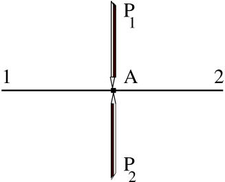
FIG. 5.: A wire with two voltage probes $P_{1}$ and $P_{2}$ at a point labeled $A$. The two probes cause phase randomization of right and left moving waves respectively.

Consider Fig. 5 in which there is a wire with two ends labeled as 1 and 2. At some point labeled $A$ in the middle of the wire, there are two wires $P_{1}$ and $P_{2}$ which are voltage probes, i.e., the net outgoing currents at each of these wires is zero. The four-wire junction at $A$ is governed by an $S$-matrix of the form

$$S~{}=~{}\left(\begin{array}[]{cccc}0&\sqrt{1-p}&0&-\sqrt{p}\\ \sqrt{1-p}&0&-\sqrt{p}&0\\ \sqrt{p}&0&\sqrt{1-p}&0\\ 0&\sqrt{p}&0&\sqrt{1-p}\end{array}\right)~{},$$ (52)

where the columns and rows carry the indices 1, 2, $P_{1}$ and $P_{2}$ in that order, and $p$ is a real parameter which lies in the range $0\leq p\leq 1$. (If $p=0$, the voltage probes have no effect, and phase randomization does not occur). A wave traveling right from end 1 can go partially out into $P_{1}$ and partially on to end 2; the part which goes out into $P_{1}$ can re-enter the wire and go on to 2. We now impose the phase randomization condition that the wave which goes out into $P_{1}$ can re-enter the wire with an arbitrary phase change of $\phi_{1}$, but it must have the same magnitude; this is necessary to ensure the zero current condition since $P_{1}$ is a voltage probe. Upon solving a problem in which there is an incoming wave of unit amplitude at end 1, and no incoming wave at end 2, we find that there is complete transmission of the wave across the point $A$. To be explicit, we take the incoming and outgoing waves at $A$ to be of the forms

$$\psi_{I}~{}=~{}\left(\begin{array}[]{c}1\\ 0\\ e^{i\phi_{1}}\psi\\ 0\end{array}\right)\quad{\rm and}\quad\psi_{O}~{}=~{}\left(\begin{array}[]{c}0\\ t\\ \psi\\ 0\end{array}\right)$$ (61)

respectively. We then use the scattering matrix in Eq. (52) to relate $\psi_{I}$ and $\psi_{O}$. On eliminating $\psi$, we find that the transmission amplitude across $A$ is given by

$$t~{}=~{}-~{}e^{i\phi_{1}}~{}\frac{1~{}-~{}\sqrt{1-p}~{}e^{-i\phi_{1}}}{1~{}-~{}\sqrt{1-p}~{}e^{i\phi_{1}}}~{},$$ (62)

so that $|t|=1$. When we calculate any physical quantity (such as a transmission or reflection probability), we will integrate over $\phi_{1}$ from 0 to $2\pi$. The following identity will prove to be useful,

$$\int_{0}^{2\pi}~{}\frac{d\phi_{1}}{2\pi}~{}t^{n}~{}=~{}(1-p)^{|n|/2}$$ (63)

for any integer $n$. As shown below, the integration over $\phi_{1}$ reduces the coherence of a wave moving to the right from 1 to 2. Similarly, we can introduce a phase change of $\phi_{2}$ for a wave which leaves and re-enters the wire at the probe $P_{2}$; integrating over $\phi_{2}$ reduces the coherence of a wave moving to the left from 2 to 1. For both right and left moving waves, the degree of coherence depends on the value of the parameter $p$ as we will now see.

We consider two waves which travel $n_{1}$ and $n_{2}$ times respectively through the point $A$ from left to right. Let us suppose that their amplitudes are $a_{1}$ and $a_{2}$ respectively in the absence of phase randomization, i.e., for $p=0$. In the presence of phase randomization, their amplitudes will be $a_{1}t^{n_{1}}$ and $a_{2}t^{n_{2}}$ respectively, where $t$ is given in Eq. (62). If these two waves contribute to a transmission probability $T$, the cross-term coming from their interference will be given by $a_{1}^{*}a_{2}t^{n_{2}-n_{1}}+a_{2}^{*}a_{1}t^{n_{1}-n_{2}}$. We now integrate this expression over the variable $\phi_{1}$. Using Eq. (63), we find that

$$\int_{0}^{2\pi}~{}\frac{d\phi_{1}}{2\pi}~{}[~{}a_{1}^{*}a_{2}~{}t^{n_{2}-n_{1}}~{}+~{}a_{2}^{*}a_{1}~{}t^{n_{1}-n_{2}}~{}]$$ (64)

$$=~{}(~{}a_{1}^{*}a_{2}~{}+~{}a_{2}^{*}a_{1}~{})~{}(1-p)^{|n_{1}-n_{2}|/2}~{}.$$ (65)

We thus see that the phase randomization has the effect of multiplying the interference of two terms by a factor which interpolates between 1 (i.e., complete phase coherence between the two waves) for $p=0$ and 0 (i.e., no phase coherence) for $p=1$. Further, the interpolating factor depends exponentially on $|n_{1}-n_{2}|$ which is proportional to the difference between the path lengths of the two waves.

Now we have to implement this idea in the systems of interest to us. We do this by generalizing the idea of phase randomization at a single point to phase randomization at a continuum of points. Let us assume that the density of such points in a wire is given by $\mu/L_{T}$, where $\mu$ is some dimensionless number (which is independent of any temperature or length scale), and that the parameter $p$ is the same at each of those points. This assumption for the density is motivated by our identification of $L_{T}$ as the phase relaxation length; the smaller the value of $L_{T}$, the more frequently phase relaxation should occur as an electron travels along the wire. Thus the number of phase relaxation points in an interval of length $L$ is equal to $\mu L/L_{T}$. Following arguments similar to the one described above, one can show that the interference of two waves which pass through that length interval $n_{1}$ and $n_{2}$ times will get multiplied by the factor $(1-p)^{|n_{1}-n_{2}|\mu L/(2L_{T})}$. If we write $(1-p)^{\mu/2}=e^{-\nu}$, where $\nu$ is a positive dimensionless number, we see that the interference between two waves whose path lengths differ by $\Delta L=|n_{1}-n_{2}|L$ will carry a factor of

$$F~{}=~{}\exp~{}[~{}-~{}\nu~{}\frac{\Delta L}{L_{T}}~{}]~{}.$$ (66)

The high temperature limit ($L_{T}\rightarrow 0$) corresponds to the incoherent case in which we ignore the interference between paths with any finite length difference; namely, we simply add up the probabilities contributed by different paths.

In our calculations of the transmission probabilities described in Secs. IV-VI, we will require an interpolating factor as in Eq. (66) only for the case $L_{T}\leq L_{S}$. It is only in that regime that our systems have more than one junction which allows for a number of different paths between any pair of long wires. For $L_{T}>L_{S}$, each of our systems effectively simplify to a system which has only one junction and, therefore, only one possible path between any pair of long wires. Hence there will be no need to consider any interference terms for $L_{T}>L_{S}$. In order to make our expressions for the transmission probabilities match as we approach $L_{T}=L_{S}$ from above and below, we will use an interpolating factor $F$ which is 1 at $L_{T}=L_{S}$. We will therefore use a formula which is motivated by the expression in Eq. (66) (with $\nu$ set equal to 1), but which is somewhat modified so that it is goes to 1 as $L_{T}$ approaches $L_{S}$ from below. We will use the following prescription,

$$F~{}=~{}\exp~{}[~{}\frac{\Delta L}{L_{S}}~{}-~{}\frac{\Delta L}{L_{T}}~{}]\quad{\rm for}\quad L_{T}\leq L_{S}~{},$$ (67)

for the factor multiplying the interference of two paths differing in length by $\Delta L$.

IV The Stub System

We will now use the ideas developed in the previous two sections to study the transmission probability of the stub system shown in Fig. 1. The $3\times 3$ scattering matrix, called $S_{3D}$, which governs the junction labeled $A$ will be assumed to be of the form given in Eq. (19-22), with complete symmetry between the two long wires labeled 1 and 3. At the other end of the stub labeled $B$, we will assume a hard wall boundary condition, i.e., perfect reflection with a phase change of $-1$.

We first consider the RG flow of the transmission probabilities $T_{ij}$. There is only one independent quantity to consider in this system, namely, $T_{13}$; all the others are related to it by Eq. (36). As outlined in Sec. II, we start from the length scale $d$ and initially use Eq. (23) to see how the various entries of $S_{3D}$ flow as functions of the length. If $L_{T}<L_{S}$, we follow this flow up to the length scale $L_{T}$ and then stop there. At that point, we compute $T_{13}$ as explained below.

If $L_{T}>L_{S}$, we first use Eq. (23) to follow the flow up to the length scale $L_{S}$. At that point, we switch over to a $2\times 2$ scattering matrix $S_{2D}$ which can be obtained from the matrix $S_{3D}$ that we get at that length scale from the RG calculation. The entries of $S_{2D}(L_{S})$ and $S_{3D}(L_{S})$ can be shown to be related as follows,

$$(S_{2D})_{11} = (S_{2D})_{33}~{}=~{}r^{\prime}~{}-~{}\frac{t^{2}\eta}{1~{}+~{}r\eta}~{},$$ (68)

$$(S_{2D})_{13} = (S_{2D})_{31}~{}=~{}t^{\prime}~{}-~{}\frac{t^{2}\eta}{1~{}+~{}r\eta}~{}.$$ (69)

where

$$\eta~{}=~{}e^{i2k_{F}L_{S}}~{}.$$ (70)

Eq. (69) will be derived in the next paragraph. [The phase factor $\eta$ appears because the electrons are assumed to have a momentum of $k_{F}$ in all regions; hence the wave functions have factors of $\exp(ik_{F}x)$.] Having obtained $S_{2D}$ at the length scale $L_{S}$, we then continue with the RG flow of that matrix following Eq. (14). This flow is stopped when we reach the length scale $L_{T}$. At that point, we compute $T_{13}$ as explained below.

Eq. (69) can be derived in one of two ways. The first way is to assume an incoming wave with unit amplitude on wire 1 and no incoming wave on wire 3, and then use the scattering matrix $S_{3D}$ at junction $A$ and the sign change at $B$. The second way, which is more instructive for us and is also easier, is to sum over all the paths that an electron can take. For instance, if we consider the different paths which go through the stub, we see that they are characterized by an integer $n=0,1,\cdots$ which is the number of times a path goes up and down the stub. The length of a path which goes from a point just to the left of $A$ to itself after going up and down the stub $n$ times is given by $2nL_{S}$. Summing over all such paths leads to the expression

$$(S_{2D})_{11} = r^{\prime}-t\eta t+t\eta r\eta t-t\eta r\eta r\eta t+\cdots$$ (71)

$$= r^{\prime}~{}-~{}\frac{t^{2}\eta}{1~{}+~{}r\eta}~{},$$ (72)

which is the first equation in Eq. (69). Similarly, we can derive the second equation in Eq. (69) by summing over all the paths which go from a point just to the left of $A$ to a point just to the right of $A$

Let us now calculate the transmission probability $T_{13}$. If $L_{T}\leq L_{S}$, we have to use $S_{3D}$ to compute an expression for $T_{13}$ with an interpolating factor $F$ as in Eq. (67). This is easy to do since we have already found the sum over all the paths as in Eq. (72). According to the phase randomization idea discussed in Sec. III, the interference between two paths characterized by integers $n_{1}$ and $n_{2}$ must be multiplied by a factor $F=f^{|n_{1}-n_{2}|}$, where

$$f~{}=~{}\exp~{}[~{}2~{}(~{}1~{}-~{}\frac{L_{S}}{L_{T}}~{})~{}]~{}.$$ (73)

This follows from the prescription Eq. (67) since the difference in path lengths is given by $\Delta L=2|n_{1}-n_{2}|L_{S}$. On summing up all the terms with the appropriate factors of $f$, we find that

$$T_{13} = t^{\prime 2}~{}+~{}\frac{t^{2}}{2}$$ (75)

$$-~{}t^{2}~{}(~{}t^{\prime}~{}+~{}\frac{r^{\prime}}{2}~{})~{}[~{}\frac{\eta f}{1+r\eta f}+\frac{\eta^{*}f}{1+r\eta^{*}f}~{}]~{},$$

where we have used some of the relations in Eq. (22). Eq. (75) is the desired interpolating expression for $T_{12}$. If we set $f=0$ (as we must do for $L_{T}<<L_{S}$), we get the incoherent expression

$$T_{13}~{}=~{}t^{\prime 2}~{}+~{}\frac{t^{2}}{2}~{}=~{}1~{}+~{}r^{\prime}~{},$$ (76)

which is independent of $\eta$. On the other hand, if we set $f=1$ (as we must do at $L_{T}=L_{S}$), we get the coherent expression

$$T_{13}~{}=~{}|~{}t^{\prime}~{}-~{}\frac{t^{2}\eta}{1~{}+~{}r\eta}~{}|^{2}$$ (77)

which is just the square of the modulus of $(S_{2D})_{13}$ given in Eq. (69). Eq. (75) interpolates between the coherent and incoherent expressions depending on the value of $f$.

There is a way of directly obtaining the incoherent expression in Eq. (76) without summing over paths. We will present this derivation here; as discussed in the next section, a similar derivation will work for the ring system where it is difficult to classify the different paths in a convenient way and therefore to sum over them. The idea is to add probabilities (intensities) rather than amplitudes. Consider a situation with the following kinds of waves: a wave of unit intensity which comes into the system from wire 1, a wave of intensity $i_{r}$ which is reflected back to wire 1, a wave of intensity $i_{t}$ which is transmitted to wire 3, a wave of intensity $i_{u}$ which travels up along the stub 2, and a wave of intensity $i_{d}$ down along the stub. [Note that the last four waves are actually made up of sums of several waves obtained after repeated travels up and down the stub; however, we will not need to explicitly sum over all those paths in this way of doing the calculation. The summation over paths will be implicit because we are assuming that $i_{r}$, $i_{t}$ and $i_{u}$ and $i_{d}$ denote the total intensities of those four kinds of waves.] Now we use the matrix $S_{3D}$ at junction $A$. This gives the following relations between these intensities,

$$i_{r} = r^{\prime 2}~{}+~{}t^{2}i_{d}~{},$$ (78)

$$i_{t} = t^{\prime 2}~{}+~{}t^{2}i_{d}~{},$$ (79)

$$i_{u} = t^{2}~{}+~{}r^{2}i_{d}~{}.$$ (80)

Similarly, the total reflection at the end $B$ implies that $i_{u}=i_{d}$. Putting these relations together, we obtain

$$i_{t}~{}=~{}1~{}+~{}r^{\prime}~{},$$ (81)

which agrees with the expression in Eq. (76).

When $L_{T}$ becomes equal to $L_{S}$, $T_{12}(L_{S})$ is equal to $|(S_{2D})_{12}|^{2}$ where $(S_{2D})_{12}$ is given in Eq. (69). [Our formalism is designed to ensure that we get the same value of $T_{13}$ at $L_{T}=L_{S}$ whether we approach that point from the high temperature or the low temperature side.] Using the parametrization in Eq. (12) and the RG equations in Eq. (14), we see that $\lambda$ at a length scale $L_{T}>L_{S}$ is related to its value at the length scale $L_{S}$ as follows,

$$\lambda(L_{T})~{}=~{}\Bigl{(}~{}\frac{L_{T}}{L_{S}}~{}\Bigr{)}^{\alpha}~{}\lambda(L_{S})~{}.$$ (82)

Then $T_{13}(L_{T})$ is given by $1/(1+\lambda^{2}(L_{T}))$.

In the coherent regime given by $L_{T}>L_{S}$, we observe that $T_{13}$ is equal to 1 if $\eta=-1$ and 0 if $\eta=1$; this follows on using Eqs. (22) and (77). We will call these resonances and anti-resonances respectively; they arise due to interference between the different paths. For these two special values of $\eta$, $T_{13}$ remains stuck at 1 and 0 and does not flow under RG. For any other value of $\eta$, $T_{13}$ starts at a value which is less than 1; it then flows towards zero till the RG evolution stops at the length scale $L_{T}$. Note that by changing the electron momentum $k_{F}$ (this can be done by changing the gate voltage), we can vary the value of $\eta$ and therefore of the matrix elements in Eq. (69); we can therefore, in principle, tune the system to resonance. [This is in contrast to a single wire system with an impurity where one can change the matrix elements of $S_{2D}$ only by varying the strength of the impurity potential which may not be easy to do experimentally.]

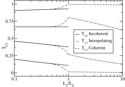
FIG. 6.: $T_{13}$ for the stub system as a function of $L_{T}/L_{S}$ for $\alpha=0.2$, $L_{S}/d=10$, $\eta=e^{i\pi/2}$, and different values of $r^{\prime}$. The four sets of curves are for $r^{\prime}=-0.10,-0.33,-0.54$ and $-0.80$ from top to bottom.

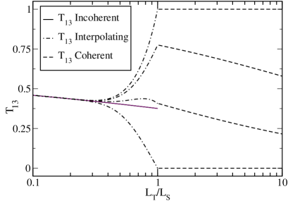
FIG. 7.: $T_{13}$ as a function of $L_{T}/L_{S}$ for $\alpha=0.2$, $L_{S}/d=10$, $r^{\prime}=-0.54$, and different values of $\eta$. The four sets of curves are for $\eta=-1,e^{i0.8\pi},e^{i0.6\pi}$ and 1 from top to bottom.

In Figs. 6-7, we show $T_{13}$ as a function of $L_{T}/L_{S}$ for various values of $r^{\prime}$ and $\eta$, with $\alpha=0.2$ on all the three wires, and $L_{S}/d=10$. In Fig. 6, we have considered four different values of $r^{\prime}$. Of these values, the first one is greater than the unstable fixed point value of $-1/3$ given in Eq. (24), the second is equal to $-1/3$, and the last two are less than $-1/3$. In the incoherent regime, we see that $T_{13}$ increases in the first case, does not change in the second case, and decreases in the last two cases. In Fig. 7, we show $T_{13}$ as a function of $L_{T}/L_{S}$ for four different values of $\eta$. In the coherent regime, we see that $T_{13}$ remains stuck at 1 and 0 for $\eta=-1$ and 1 respectively, while it decreases for the other two cases. It is clear that modifying $\eta$ (by changing the gate voltage) can lead to large changes in $T_{13}$ in the coherent regime.

V The Ring System

We now turn to the ring system shown in Fig. 2. We will assume that both the junctions $A$ and $B$ are described by the same $3\times 3$ scattering matrix $S_{3D}$ given in Eqs. (19-22), with complete symmetry between the two arms of the ring labeled 2 and 4.

The RG evolution of the transmission probabilities $T_{ij}$ is studied in the same way as for the stub system. (Once again, there is only one independent quantity to consider here, namely, $T_{13}$; the others are related to it by Eq. (36)). We start from the length scale $d$ and initially use Eq. (23) to see how the various entries of the two matrices $S_{3D}$ flow as functions of the length. If $L_{T}<L_{S}$, we follow this flow up to the length scale $L_{T}$ and then stop there. At that point, we compute $T_{13}$ as explained below.

If $L_{T}>L_{S}$, we first use Eq. (23) to follow the flow up to the length scale $L_{S}$. At that point, we switch over to a $2\times 2$ scattering matrix $S_{2D}$ which can be obtained from the matrix $S_{3D}$ that we get at that length scale from the RG calculation. For the ring system, the off-diagonal matrix elements of $S_{2D}(L_{S})$ are related to the parameter $r^{\prime}$ appearing in $S_{3D}(L_{S})$ as follows [8].

$$(S_{2D})_{13}~{}=~{}(S_{2D})_{31}$$ (83)

$$=~{}\frac{2\cos(\Phi/2)~{}\eta^{1/2}~{}(1~{}-~{}\eta)~{}(-2r^{\prime})~{}(1~{}+~{}r^{\prime})}{[1~{}+~{}(1+2r^{\prime})\eta]^{2}~{}-~{}2(1~{}+~{}r^{\prime})^{2}~{}(1~{}+~{}\cos\Phi)~{}\eta}~{},$$ (84)

(85)

where $\eta=e^{i2k_{F}L_{S}}$, and $\Phi$ is a dimensionless number which is related to the magnetic flux $\phi_{B}$ enclosed by the ring through the expression

$$\Phi~{}=~{}\frac{e\phi_{B}}{\hbar c}~{}.$$ (86)

Eq. (85) will be derived in the Appendix. Having obtained $S_{2D}$ at the length scale $L_{S}$, we continue with the RG flow following Eq. (14). The flow is stopped when we reach the length scale $L_{T}$. At that point, we compute $T_{13}$ as explained below.

As shown in the Appendix, Eq. (85) can be obtained by assuming an incoming wave with unit amplitude on wire 1 and no incoming wave on wire 3, and then using the scattering matrices at junctions $A$ and $B$ [8]. One might think of deriving Eq. (85) by summing over all paths which go from wire 1 to wire 3, just as we did for the stub system. However, it seems very hard to enumerate the set of paths for the ring system in a convenient way. This is because there are two arms, and a path can go into either one of the two arms every time it encounters one of the two junctions.

This difficulty in summing over paths also makes it hard to find a simple interpolating formula for the conductance in the regime $L_{T}<L_{S}$. To see this more clearly, we first note that in the stub system, two paths which have equal lengths must necessarily be identical to each other. Any point which phase randomizes waves moving in one particular direction will therefore occur the same number of times in the two paths. Hence, the interference between the two paths will not come with any powers of either the phase factor $\eta$ or the phase randomization factor $f$. If there are two paths of unequal lengths $2n_{1}L_{S}$ and $2n_{2}L_{S}$ in the stub system, then any point which phase randomizes waves moving in a particular direction point will occur $n_{1}$ times in one path and $n_{2}$ times in the other path. Therefore the interference between the two paths will come with a factor of $\eta^{n_{1}-n_{2}}f^{|n_{1}-n_{2}|}$. Thus, the power of $\eta$ and the power of $f$ are always related to each other in a simple way. (This is why a factor of $f$ always accompanies a factor of $\eta$ or $\eta^{*}$ in Eq. (75)). The situation is quite different in the ring system. Here the powers of $\eta$ and $f$ are not necessarily related to each other in any simple way. For instance, consider a path which enters the system through wire 1, goes into the arm 2 and leaves through wire 3, and a second path which enters through wire 1, goes into the arm 4 and leaves through wire 3. These two paths have the same length $L_{S}$; the interference between the two will therefore not carry any powers of $\eta$. However, a phase randomization point which lies on one path will not lie on the other path. Hence, the phase randomizations will not cancel between the two paths, and the interference between the two paths will carry a factor of $f$. Thus, there is no general relation between the power of $\eta$ and the power of $f$. This makes is difficult to find an interpolating expression for $T_{13}$.

Even though we do not have an interpolating expression for the ring system, we can obtain an incoherent expression for $T_{13}$ by following a procedure similar to the one we used for the stub system. The idea again is to add probabilities rather than amplitudes. Consider a situation with the following kinds of waves: a wave of unit intensity which comes into the system from wire 1, a wave of intensity $i_{r}$ which is reflected back to wire 1, a wave of intensity $i_{t}$ which is transmitted to wire 3, waves of intensity $i_{2r}$ and $i_{2l}$ which travel respectively from junction $A$ to junction $B$ and vice versa along wire 2, and waves of intensity $i_{4r}$ and $i_{4l}$ which travel respectively from junction $A$ to junction $B$ and vice versa along wire 4. [Note as before that the last six waves are actually made up of sums of several waves obtained after repeated bounces from the two junctions. We do not need to explicitly sum over all these paths because we are assuming that $i_{r},i_{t},\cdots$ denote the total intensities of these six kinds of waves.] Now we use the matrices at junctions $A$ and $B$. This gives the following relations between the various intensities,

$$i_{r} = r^{2}~{}+~{}t^{2}~{}(~{}i_{2l}~{}+~{}i_{4l}~{})~{},$$ (87)

$$i_{t} = t^{2}~{}(~{}i_{2r}~{}+~{}i_{4r}~{})~{},$$ (88)

$$i_{2r} = t^{2}~{}+~{}r^{\prime 2}i_{2l}~{}+~{}t^{\prime 2}i_{4l}~{},$$ (89)

$$i_{4r} = t^{2}~{}+~{}r^{\prime 2}i_{4l}~{}+~{}t^{\prime 2}i_{2l}~{},$$ (90)

$$i_{2l} = r^{\prime 2}i_{2r}~{}+~{}t^{\prime 2}i_{4r}~{},$$ (91)

$$i_{4l} = r^{\prime 2}i_{4r}~{}+~{}t^{\prime 2}i_{2r}~{}.$$ (92)

Solving these equations and using some of the relations in Eq. (22), we find the incoherent expression for $T_{13}$ (valid for $L_{T}<<L_{S}$) to be

$$i_{t}~{}=~{}-~{}\frac{2r^{\prime}~{}(1~{}+~{}r^{\prime})}{1~{}+~{}r^{\prime}~{}+~{}r^{\prime 2}}~{}.$$ (93)

which is independent of both $\eta$ and $\Phi$.

At the point $L_{T}=L_{S}$, $T_{13}(L_{S})$ is given by $|(S_{2D})_{13}|^{2}$ where $(S_{2D})_{13}$ is given in Eq. (85). We can again use the parametrization in Eq. (12) and the RG equation in Eq. (14) to we obtain $T_{13}(L_{T})=1/(1+\lambda^{2}(L_{T}))$, where $\lambda(L_{T})$ is given in Eq. (82).

In Fig. 8, we show $T_{13}$ as a function of $L_{T}/L_{S}$ for various values $\eta$, with $\alpha=0.2$ on all the wires, and $L_{S}/d=10$.

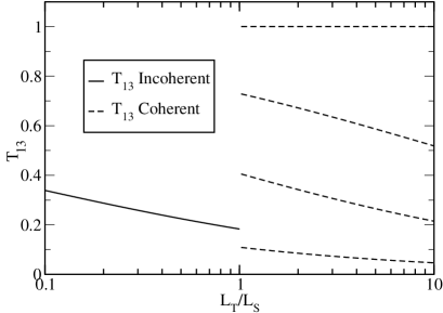
FIG. 8.: $T_{13}$ for the ring system as a function of $L_{T}/L_{S}$ for $\alpha=0.2$, $L_{S}/d=10$, $r^{\prime}=-0.18$, $\Phi=0$, and different values of $\eta$. The four coherent curves are for $\eta=1,e^{i0.08\pi},e^{i0.16\pi}$ and $e^{i0.4\pi}$ from top to bottom. The incoherent curve is the same for all $\eta$.

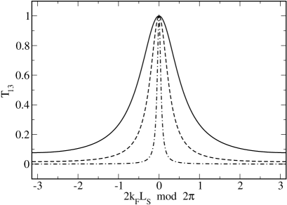
FIG. 9.: $T_{13}$ as a function of $2k_{F}L_{S}$ for $\alpha=0.2$, $L_{S}/d=10$, $r^{\prime}=-0.19$, $\Phi=0$, and different values of $L_{T}/L_{S}$. The three sets of curves are for $L_{T}/L_{S}=1,50$ and $10^{5}$ from top to bottom.

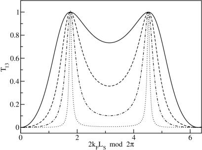
FIG. 10.: $T_{13}$ as a function of $2k_{F}L_{S}$ for $\alpha=0.2$, $L_{S}/d=10$, $\Phi=0.5\pi$, and different values of $L_{T}/L_{S}$. The four sets of curves are for $L_{T}/L_{S}=1,50,3000,$ and $10^{6}$ from top to bottom. Note that there is a transmission zero at $2k_{F}L_{S}=0$ mod $2\pi$.

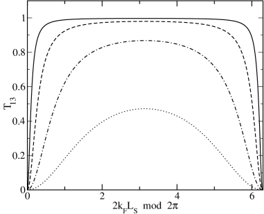
FIG. 11.: $T_{13}$ as a function of $2k_{F}L_{S}$ for $\alpha=0.2$, $L_{S}/d=10$, $\Phi=0$, and different values of $L_{T}/L_{S}$. The four sets of curves are for $L_{T}/L_{S}=1,150,20000$ and $10^{6}$ from top to bottom. Note that there is a transmission zero at $2k_{F}L_{S}=0$ mod $2\pi$.

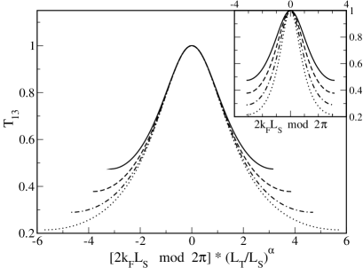
FIG. 12.: $T_{13}$ as a function of the scaled variable $[2k_{F}L_{S}$ mod $2\pi]~{}(L_{T}/L_{S})^{\alpha}$ for $\alpha=0.2$, $L_{S}/d=10$, $r^{\prime}=-0.32$, $\Phi=0$, and different values of $L_{T}/L_{S}$. The four sets of curves are for $L_{T}/L_{S}=1,2.7,7.4$ and $20$ from top to bottom. The inset shows the same plots without scaling, i.e., $T_{13}$ as a function of $2k_{F}L_{S}$.

In the coherent regime given by $L_{T}>L_{S}$, we can find the conditions under which there are resonances and anti-resonances in the transmission through the ring, i.e., $T_{13}=1$ and 0 respectively. (Some of these conditions have been discussed in Ref. [8]). We find that $T_{13}=1$ for the following values of $\eta,e^{i\Phi}$ and $r^{\prime}$.

(i) $\eta=e^{i\Phi}=1$, and $r^{\prime}$ can take any value. Note that for these values of $\eta$ and $e^{i\Phi}$, there are eigenstates of the electron which are confined to the ring.

(ii) $\eta=e^{\pm i\Phi}$, and $r^{\prime}=0$. For this relation between $\eta$ and $e^{i\Phi}$, there are eigenstates of the electron on the ring. Further, $r^{\prime}=0$ implies $t=0$ which means that these eigenstates cannot escape from the ring to the long wires.

(iii) $e^{i\Phi}=1$, $r^{\prime}=-1/2$, and $\eta$ can take any value. Note that $r^{\prime}=-1/2$ implies $r=0$ which means that a wave which is coming in on wire 1 (3) suffers no reflection at junction $A$ ($B$).

[We note that both the numerator and denominator of Eq. (85) vanish under conditions (i) and (ii); hence one has to take the limit appropriately to see that $T_{13}=1$.]

Similarly, we find that $T_{13}=0$ for the following values of $\eta$, $e^{i\Phi}$ and $r^{\prime}$.

(i) $\eta=1$, and $e^{i\Phi}$ and $r^{\prime}$ can take any values except 1 and -1 respectively.

(ii) $r^{\prime}=0$, and $\eta$ and $e^{i\Phi}$ can take any values except $\eta=e^{\pm i\Phi}$. Note that $r^{\prime}=0$ implies that $t=0$ which means that there is no transmission between the long wires and the ring.

(iii) $r^{\prime}=-1$, and $\eta$ can take any value except 1, while $e^{i\Phi}$ can take any value. Once again, $r^{\prime}=-1$ implies that $t=0$ which means that there is no transmission between the long wires and the ring.

(iv) $e^{i\Phi}=-1$, and $(\eta,r^{\prime})$ can take any values except $(1,-1)$ and $(-1,0)$.

As in the stub system, if $T_{13}$ begins with the value 1 or 0 at $L_{T}/L_{S}=1$, it remains stuck there and does not flow under RG as we go to larger length scales. For any other starting value of $T_{13}$, it flows towards zero till the RG evolution stops at the length scale $L_{T}$. It is interesting to consider the shape of the resonance line which is a plot of $T_{13}$ versus the momentum $k_{F}$ (or, equivalently, $\eta$) at very low temperatures. As discussed in the following paragraph, one finds that the line shape becomes narrower with decreasing temperature, with the width at half maximum scaling with temperature as $T^{\alpha}$. Figs. 9-10 show this feature qualitatively for the resonances of types (i) and (ii) described above. In Fig. 10, we see pairs of resonances because $T_{13}$ has maxima at $2k_{F}L_{S}$ equal to $\Phi$ and $-\Phi$ mod $2\pi$. Fig. 11 shows the resonance of type (iii). Here $T_{13}$ is close to 1 for a wide range of $k_{F}$ (or $\eta$) at $L_{T}/L_{S}=1$; this is consistent with the resonance condition given in (iii) above. We also observe anti-resonances ($T_{13}=0$) in Figs. 10 and 11 at $2k_{F}L_{S}=0$ mod $2\pi$.

Let us now discuss the resonance line shape in more detail. Exactly at a resonance, occuring at, say, $k_{F}=k_{F0}$, $T_{13}$ is equal to 1, and it remains stuck at that value no matter how large $L_{T}$ is. We can now ask: what is the shape of the resonance line slightly away from $k_{F}=k_{F0}$ ? If one deviates from $k_{F0}$ by a small amount $\Delta k=|k_{F}-k_{F0}|$ which is fixed, one finds that the transmission $T_{13}$ differs from 1 by an amount of order $(\Delta k)^{2}$. (An example of this is discussed below). Comparing this with the form in Eq. (12), we see that $\lambda\sim\Delta k$ at the length scale $L_{S}$. Eq. (14) then implies that $\lambda$ will grow as $\Delta k(L_{T}/L_{S})^{\alpha}$ at low temperature; hence $T_{13}$ will approach zero as $1/\lambda^{2}\sim T^{2\alpha}$ at very low temperature, if $\Delta k$ is held fixed. On the other hand, the width of the resonance line at half the maximum possible value of $T_{13}$ is given by the condition that $\Delta k(L_{T}/L_{S})^{\alpha}\sim 1$, which implies that $\Delta k\sim T^{\alpha}$. Thus the resonance line becomes narrower with decreasing temperature, with a width $\Delta k$ which vanishes as $T^{\alpha}$. To summarize, $T_{13}$ depends on the variables $\Delta k$ and $T$ through the combination $x=\Delta k/T^{\alpha}$, and $T_{13}(x)\sim 1/x^{2}$ as $x\rightarrow\infty$. (This agrees with the expression given in Ref. [13] for small values of $\alpha$). As a specific example, let us consider the resonance of type (i). We set $e^{i\Phi}=1$ and take the limit $k_{F}\rightarrow k_{F0}=\pi n/L_{S}$ in Eq. (85). We find that at the length scale $L_{S}$,

$$T_{13}~{}=~{}1~{}-~{}\frac{(1+2r^{\prime})^{2}}{16r^{\prime 2}~{}(1+r^{\prime})^{2}}~{}(2\Delta kL_{S})^{2}$$ (94)

up to order $(\Delta k)^{2}$. Eq. (14) then implies that at the length scale $L_{T}$,

$$T_{13}~{}=~{}\Bigl{[}~{}1~{}+~{}\frac{(1+2r^{\prime})^{2}}{16r^{\prime 2}~{}(1+r^{\prime})^{2}}~{}(2\Delta kL_{S})^{2}(\frac{L_{T}}{L_{S}})^{2\alpha}~{}\Bigr{]}^{-1}~{}.$$ (95)

Thus, if $r^{\prime}$ is held fixed and $T_{13}$ is plotted against $\Delta k(L_{T}/L_{S})^{\alpha}$, we should get the same curve for different values of $L_{T}/L_{S}$, provided that the quadratic approximation in Eq. (94) holds good. In Fig. 12, we show $T_{13}$ as a function of $2\Delta kL_{S}(L_{T}/L_{S})^{\alpha}$ for four different values of $L_{T}/L_{S}$. We see that the curves agree well with each other down to about $T_{13}=0.7$. For comparison, we have shown the same plots without scaling in the inset; we see that they begin disagreeing below $T_{13}=0.95$. (We find similar resonance line shapes in the stub and four-wire systems, although we have not shown those plots in this paper).

VI The Four-wire System

Finally, let us consider the four-wire system shown in Fig. 3. We will assume that both the junctions $A$ and $B$ are described by the same $3\times 3$ scattering matrix $S_{3D}$ given in Eqs. (19-22), with complete symmetry between the wires 1 and 2 on one side and the wires 3 and 4 on the other side. The transmission probabilities enjoy the symmetries described in Eq. (42).

We first consider the RG flow of the transmission probabilities $T_{ij}$. Due to the symmetries of the system, and the relations in Eqs. (33-34), we see that there are only two independent quantities to consider, namely, $T_{12}$ and $T_{13}$. Following the formalism in Sec. II, we start from the length scale $d$ and initially use Eq. (23) to see how the various entries of $S_{3D}$ flow as functions of the length. If $L_{T}<L_{S}$, we follow this flow up to the length scale $L_{T}$, and then compute $T_{12}$ and $T_{13}$.

If $L_{T}>L_{S}$, we first use Eq. (23) to follow the flow up to the length scale $L_{S}$. At that point, we switch over to a $4\times 4$ scattering matrix $S_{4D}$ which can be obtained from the matrix $S_{3D}$ that we get at that length scale from the RG calculation. The entries of $S_{4D}(L_{S})$ and $S_{3D}(L_{S})$ can be shown to be related as follows,

$$(S_{4D})_{11} = r^{\prime}~{}+~{}\frac{t^{2}r\eta}{1~{}-~{}r^{2}\eta}~{},$$ (96)

$$(S_{4D})_{12} = t^{\prime}~{}+~{}\frac{t^{2}r\eta}{1~{}-~{}r^{2}\eta}~{},$$ (97)

$$(S_{4D})_{13} = \frac{t^{2}\eta^{1/2}}{1~{}-~{}r^{2}\eta}~{}.$$ (98)

where $\eta=e^{i2k_{F}L_{S}}$. (Eq. (98) will be derived in the next paragraph). Having obtained $S_{4D}$ at the length scale $L_{S}$, we then continue with the RG flow of that matrix using Eq. (6). This flow is stopped when we reach the length scale $L_{T}$, where we compute $T_{12}$ and $T_{13}$.

As in the stub system, Eq. (98) can be derived in one of two ways. The first way is to assume an incoming wave with unit amplitude on wire 1 and no incoming waves on wires 2, 3 and 4, and then use the scattering matrices $S_{3D}$ at junctions $A$ and $B$. The second way is to sum over all the paths that an electron can take. As in the stub system, the different paths going between any two of the long wires $i$ and $j$ are characterized by an integer $n=0,1,\cdots$ which is the number of times a path goes right and left on the central wire labeled 5. For instance, the sum over paths which go from a point on wire 1 lying very close to the junction $A$ to itself gives the series

$$(S_{4D})_{11} = r^{\prime}~{}+~{}t\eta^{1/2}r\eta^{1/2}t$$ (100)

$$+~{}t\eta^{1/2}r\eta^{1/2}r\eta^{1/2}r\eta^{1/2}t~{}+~{}\cdots~{},$$

which agrees with the first equation in Eq. (98). Similarly, we can derive the other expressions in Eq. (98).

Let us now calculate the transmission probabilities $T_{12}$ and $T_{13}$. If $L_{T}\leq L_{S}$, we have to use $S_{3D}$ to compute expressions for $T_{ij}$ with an interpolating factor $f$ as in Eq. (73). This is as easy to do here as in the stub system since we know how to explicitly sum over all the paths. The interference between the contributions of two paths characterized by integers $n_{1}$ and $n_{2}$ must be multiplied by a factor $f^{|n_{1}-n_{2}|}$, where $f$ is given in Eq. (73). On summing up all the terms with the appropriate factors of $f$, we find that

$$T_{12} = t^{\prime 2}~{}+~{}\frac{t^{2}r^{2}}{2(1+r^{2})}$$ (102)

$$+~{}t^{2}\Bigl{(}t^{\prime}r+\frac{r^{4}}{2(1+r^{2})}\Bigr{)}\Bigl{(}\frac{\eta f}{1-r^{2}\eta f}+\frac{\eta^{*}f}{1-r^{2}\eta^{*}f}\Bigr{)},$$

$$T_{13} = \frac{t^{2}}{2(1+r^{2})}+\frac{t^{2}r^{2}}{2(1+r^{2})}\Bigl{(}\frac{\eta f}{1-r^{2}\eta f}+\frac{\eta^{*}f}{1-r^{2}\eta^{*}f}\Bigr{)}.$$ (103)

These are the desired interpolating expressions for $T_{12}$ and $T_{13}$. If we set $f=0$ (as we must do for $L_{T}<<L_{S}$), we get the incoherent expressions

$$T_{12} = t^{\prime 2}~{}+~{}\frac{t^{2}r^{2}}{2(1+r^{2})}~{}=~{}\frac{(1+r^{\prime})(2+5r^{\prime}+4r^{\prime 2})}{2(1+2r^{\prime}+2r^{\prime 2})}~{},$$ (105)

$$T_{13} = \frac{t^{2}}{2(1+r^{2})}~{}=~{}-~{}\frac{r^{\prime}(1+r^{\prime})}{2(1+2r^{\prime}+2r^{\prime 2})}~{},$$ (106)

which are independent of $\eta$. On the other hand, if we set $f=1$ (as we must do at $L_{T}=L_{S}$), we get the coherent expressions which are given by the square of the modulus of the entries $(S_{4D})_{12}$ and $(S_{4D})_{13}$ in Eq. (98).

As in the stub system, there is a way of directly obtaining the incoherent expression in Eq. (106) without summing over paths, by adding probabilities rather than amplitudes. We consider a situation with the following kinds of waves: a wave of unit intensity which comes into the system from wire 1, waves of intensity $i_{2}$, $i_{3}$ and $i_{4}$ which go into wires 2, 3 and 4, and waves of intensity $i_{r}$ and $i_{l}$ which travel right and left respectively on wire 5. We then use the matrices $S_{3D}$ at junctions $A$ and $B$ to write down the relations between all these intensities, and then solve for $i_{2}$ and $i_{3}$. This reproduces the results in Eq. (106).

FIG. 13.: $T_{13}$ for the four-wire system as a function of $L_{T}/L_{S}$ for $\alpha=0.2$, $L_{S}/d=10$, and $\eta=1$. The four sets of curves (incoherent and interpolating) are for $r^{\prime}=-0.43,-0.28,-0.17$ and $-0.07$ from top to bottom. The coherent curve remains stuck at $1/4$ for all values of $r^{\prime}$ since $\eta=1$.

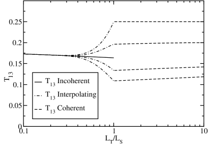
FIG. 14.: $T_{13}$ as a function of $L_{T}/L_{S}$ for $\alpha=0.2$, $L_{S}/d=10$, and $r^{\prime}=-0.28$. The four sets of curves (interpolating and coherent) are for $\eta=1,e^{i0.3\pi},e^{i0.6\pi}$ and $e^{i0.9\pi}$ from top to bottom. The incoherent curve is independent of $\eta$.

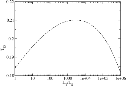
FIG. 15.: $T_{13}$ as a function of $L_{T}/L_{S}$ for $\alpha=0.2$, $L_{S}/d=10$, $r^{\prime}=-0.33$ and $\eta=e^{i0.52\pi}$. $T_{13}$ first increases and then decreases at very low temperatures.

If $L_{T}>L_{S}$, $T_{12}$ and $T_{13}$ are equal to $|(S_{4D})_{12}|^{2}$ and $|(S_{4D})_{13}|^{2}$, where $(S_{4D})_{12}$ and $(S_{4D})_{13}$ are given in Eq. (98). In this regime, the RG flow has to be carried out numerically for the reasons explained after Eq. (29). In general, we find that at long distances, $b$ and $c$ flow to zero as indicated in Eq. (30); hence $T_{12}$ and $T_{13}$ go to zero as $L^{-2\alpha}$.

In the coherent regime given by $L_{T}>L_{S}$, we observe that $T_{12}$ and $T_{13}$ are both equal to $1/4$ if either $\eta=1$ or $r^{\prime}=-1/2$. We may call these resonances since the maximum possible value of $T_{13}$ which is allowed by the form of the matrix in Eq. (29) is $1/4$. If $\eta=1$, $T_{13}$ remains stuck at $1/4$ and does not flow under RG. This can be seen in Fig. 13 where we show $T_{13}$ as a function of $L_{T}/L_{S}$ for various values of $r^{\prime}$. For any other value of $\eta$, $T_{13}$ flows till the RG evolution stops at the length scale $L_{T}$. (As discussed below, $T_{13}$ can sometimes increase before eventually decreasing towards zero at very low temperatures). As in the stub system, we can vary the value of $\eta$ and therefore tune the system to resonance by changing the electron momentum $k_{F}$.

In Fig. 14, we show $T_{13}$ as a function of $L_{T}/L_{S}$ for various values of $\eta$. In Fig. 15, we show the cross-over behavior of $T_{13}$ mentioned in Sec. II. In the coherent regime, for certain ranges of values of $r^{\prime}$ and $\eta$, $T_{13}$ first increases and then decreases at very low temperatures.

VII Discussion

In this work, we have derived the RG equations and the transmission probabilities (and conductances) for three systems of experimental interest. The RG flows and the consequent power-laws in the temperature and length dependences of the conductances are purely a result of the interactions in the wires; there is no RG flow if the interaction parameters $\alpha_{i}$ are all zero. A peculiarity of our RG formalism is that it has two stages which work in the regimes of high and low temperature respectively. We abruptly switch between the two stages when we cross the point $L_{T}/L_{S}=1$. It would be useful to develop an interpolating formalism for the RG flow which can vary smoothly across the intermediate range of temperature. In our way of deriving the RG equations, this may require an analysis of the way in which Friedel oscillations from two junctions interfere with each other.

Our results should be applicable to the systems mentioned earlier such as multi-arm quantum wires [1, 2], various kinds of carbon nanotubes [3, 4], and systems with other kinds of geometry [5, 6, 7]. While some of the early experiments focussed on electronic transport in the presence of an external magnetic field and the effects of geometry, measuring the various conductances at different temperatures (and, if possible, different wire lengths) should reveal the interaction induced power-laws discussed in our work. Note that a spread in the phase (as discussed after Eq. (31) in Sec. II) and phase randomization (as discussed in Sec. III) are the only effects of thermal fluctuations that we have considered in this work. We have ignored other effects of finite temperature, such as momentum relaxation by inelastic scattering, and corrections to the Landauer-Büttiker conductances due to thermal broadening of the Fermi-Dirac distribution near the Fermi energy. An application of our work to experiments would require one to disentangle these other features before the effects of interactions can become visible. Typically, the temperature at which these experiments are done is about $0.1-1^{o}$ K, while the Fermi energy is about $10^{o}$ K which is much larger [6]; hence the thermal broadening effect is expected to be small.

One limitation of our work is that we have assumed linear relations between the incoming and outgoing fermion fields. In principle, other interesting things can happen at a junction, particularly if we consider the case of spinful fermions and if some of the wires are superconducting rather than metallic. For instance, there may be Andreev reflection in which an electron striking the junction from one wire is reflected back as a hole while two electrons are transmitted into some of the other wires [5, 19]. It would be interesting to study these phenomena using the techniques developed in this paper.

ACKNOWLEDGMENTS

D.S. acknowledges financial support from a Homi Bhabha Fellowship and the Council of Scientific and Industrial Research, India through Grant No. 03(0911)/00/EMR-II.

APPENDIX

We will derive Eq. (85) here. We consider a situation with the following kinds of waves: an incoming wave on wire 1 whose amplitude is unity just to the left of junction $A$, an outgoing wave on wire 1 whose amplitude is $\psi_{1,{\rm out}}$ just to the left of junction $A$, an outgoing wave on wire 3 whose amplitude is $\psi_{3,{\rm out}}$ just to the right of junction $B$, waves on wires 2 and 4 which are incoming at junction $A$ and have amplitudes $\psi_{2,{\rm in}}^{A}$ and $\psi_{4,{\rm in}}^{A}$ just to the right of $A$, waves on wires 2 and 4 which are outgoing at junction $A$ and have amplitudes $\psi_{2,{\rm out}}^{A}$ and $\psi_{4,{\rm out}}^{A}$ just to the right of $A$, waves on wires 2 and 4 which are incoming at junction $B$ and have amplitudes $\psi_{2,{\rm in}}^{B}$ and $\psi_{4,{\rm in}}^{B}$ just to the left of $B$, and waves on wires 2 and 4 which are outgoing at junction $B$ and have amplitudes $\psi_{2,{\rm out}}^{B}$ and $\psi_{4,{\rm out}}^{B}$ just to the left of $B$. Our aim is to find an expression for the transmitted amplitude $\psi_{3,{\rm out}}$.

The Schrödinger equation relates many of the amplitudes introduced above to each other. This is because of the following features: a wave which travels a distance $x$ picks up a phase of $e^{ik_{F}x}$ (we are assuming that all the particles have momentum $k_{F}$), a wave which travels anticlockwise around the ring from junction $A$ to junction $B$ or vice versa picks up a phase of $e^{i\Phi/2}$, and a wave which travels clockwise around the ring from junction $A$ to junction $B$ or vice versa picks up a phase of $e^{-i\Phi/2}$. This gives us the following relations:

$$\psi_{2,{\rm in}}^{B} = e^{ik_{F}L_{S}-i\Phi/2}~{}\psi_{2,{\rm out}}^{A}~{},$$ (107)

$$\psi_{2,{\rm in}}^{A} = e^{ik_{F}L_{S}+i\Phi/2}~{}\psi_{2,{\rm out}}^{B}~{},$$ (108)

$$\psi_{4,{\rm in}}^{B} = e^{ik_{F}L_{S}+i\Phi/2}~{}\psi_{4,{\rm out}}^{A}~{},$$ (109)

$$\psi_{4,{\rm in}}^{A} = e^{ik_{F}L_{S}-i\Phi/2}~{}\psi_{4,{\rm out}}^{B}~{}.$$ (110)

Now we use the form of the scattering matrices in Eq. (19) at the two junctions. At junction $A$, we have

$$\psi_{1,{\rm out}} = r~{}+~{}t~{}(~{}\psi_{2,{\rm in}}^{A}~{}+~{}\psi_{4,{\rm in}}^{A}~{})~{},$$ (111)

$$\psi_{2,{\rm out}}^{A} = t~{}+~{}r^{\prime}\psi_{2,{\rm in}}^{A}~{}+~{}t^{\prime}\psi_{4,{\rm in}}^{A}~{},$$ (112)

$$\psi_{4,{\rm out}}^{A} = t~{}+~{}r^{\prime}\psi_{4,{\rm in}}^{A}~{}+~{}t^{\prime}\psi_{2,{\rm in}}^{A}~{}.$$ (113)

At junction $B$, we have

$$\psi_{3,{\rm out}} = t~{}(~{}\psi_{2,{\rm in}}^{B}~{}+~{}\psi_{4,{\rm in}}^{B}~{})~{},$$ (114)

$$\psi_{2,{\rm out}}^{B} = r^{\prime}\psi_{2,{\rm in}}^{B}~{}+~{}t^{\prime}\psi_{4,{\rm in}}^{B}~{},$$ (115)

$$\psi_{4,{\rm out}}^{B} = r^{\prime}\psi_{4,{\rm in}}^{B}~{}+~{}t^{\prime}\psi_{2,{\rm in}}^{B}~{}.$$ (116)

Using Eqs. (110-116), we obtain the expression for $(S_{2D})_{31}=\psi_{3,{\rm out}}$ given in Eq. (85).

REFERENCES

- [1] G. Timp, R. E. Behringer, E. H. Westerwick, and J. E. Cunningham, in Quantum Coherence in Mesoscopic Systems, edited by B. Kramer (Plenum Press, 1991) pages 113-151 and references therein; C. B. J. Ford, S. Washburn, M. Büttiker, C. M. Knoedler, and J. M. Hong, Phys. Rev. Lett. 62, 2724 (1989).
- [2] K. L. Shepard, M. L. Roukes, and B. P. Van der Gaag, Phys. Rev. Lett. 68, 2660 (1992).
- [3] C. Papadopoulos, A. Rakitin, J. Li, A. S. Vedeneev, and J. M. Xu, Phys. Rev. Lett. 85, 3476 (2000).
- [4] J. Kim, K. Kang, J.-O. Lee, K.-H. Yoo, J.-R. Kim, J. W. Park, H. M. So, and J.-J. Kim, J. Phys. Soc. Jpn. 70, 1464 (2001).
- [5] V. T. Petrashov, V. N. Antonov, P. Delsing, and R. Claeson, Phys. Rev. Lett. 70 (1993) 347.
- [6] M. Casse, Z. D. Kvon, G. M. Gusev, E. B. Olshanetskii, L. V. Litvin, A. V. Plotnikov, D. K. Maude, and J. C. Portal, Phys. Rev. B 62, 2624 (2000).
- [7] P. Debray, O. E. Raichev, P. Vasilopoulos, M. Rahman, R. Perrin, and W. C. Mitchell, Phys. Rev. B 61, 10950 (2000); R. Akis, P. Vasilopoulos, and P. Debray, ibid. 56, 9594 (1997); R. Akis, P. Vasilopoulos, and P. Debray, ibid. 52, 2805 (1995).
- [8] M. Büttiker, Y. Imry, and M. Ya. Azbel, Phys. Rev. A 30, 1982 (1984).
- [9] T. P. Pareek and A. M. Jayannavar, Phys. Rev. B 54, 6376 (1996); T. P. Pareek, P. Singha Deo, and A. M. Jayannavar, ibid. 52, 14657 (1995); P. Singha Deo and A. M. Jayannavar, ibid. 50, 11629 (1994).
- [10] Y. Shi and H. Chen, Phys. Rev. B 60, 10949 (1999).
- [11] P. Singha Deo and M. V. Moskalets, Phys. Rev. B 61, 10559 (2000); M. V. Moskalets and P. Singha Deo, ibid. 62, 6920 (2000).
- [12] T.-S. Kim, S. Y. Cho, C. K. Kim, and C.-M. Ryu, Phys. Rev. B 65, 245307 (2002).
- [13] C. L. Kane and M. P. A. Fisher, Phys. Rev. B 46, 15233 (1992).
- [14] I. Safi and H. J. Schulz, Phys. Rev. B 52, 17040 (1995); D. L. Maslov and M. Stone, ibid 52, 5539 (1995); V. V. Ponomarenko, ibid. 52, 8666 (1995).
- [15] D. L. Maslov, Phys. Rev. B, 52, 14386 (1995); A. Furusaki and N. Nagaosa, ibid 54, 5239 (1996); I. Safi and H. J. Schulz, ibid 59, 3040 (1999).
- [16] S. Lal, S. Rao, and D. Sen, Phys. Rev. Lett. 87, 026801 (2001), Phys. Rev. B 65, 195304 (2002), and cond-mat/0104402.
- [17] A. O. Gogolin, A. A. Nersesyan, and A. M. Tsvelik, Bosonization and Strongly Correlated Systems (Cambridge University Press, Cambridge, 1998); S. Rao and D. Sen, in Field Theories in Condensed Matter Physics, edited by S. Rao (Hindustan Book Agency, New Delhi, 2001).
- [18] S. Tarucha, T. Honda, and T. Saku, Sol. St. Comm. 94, 413 (1995); A. Yacoby, H. L. Stormer, N. S. Wingreen, L. N. Pfeiffer, K. W. Baldwin, and K. W. West, Phys. Rev. Lett. 77, 4612 (1996); C. -T. Liang, M. Pepper,, M. Y. Simmons, C. G. Smith, and D. A. Ritchie, Phys. Rev. B 61, 9952 (2000); B. E. Kane, G. R. Facer, A. S. Dzurak, N. E. Lumpkin, R. G. Clark, L. N. Pfeiffer, and K. W. West, App. Phys. Lett. 72, 3506 (1998); D. J. Reilly, G. R. Facer, A. S. Dzurak, B. E. Kane, R. G. Clark, P. J. Stiles, J. L. O’Brien, N. E. Lumpkin, L. N. Pfeiffer, and K. W. West, Phys. Rev. B 63, 121311 (2001).
- [19] C. Nayak, M. P. A. Fisher, A. W. W. Ludwig, and H. H. Lin, Phys. Rev. B 59, 15694 (1999).
- [20] A. Komnik and R. Egger, Phys. Rev. Lett. 80, 2881 (1998), and Eur. Phys. J. B 19, 271 (2001).
- [21] S. Lal, S. Rao, and D. Sen, Phys. Rev. B 66, 165327 (2002).
- [22] S. Chen, B. Trauzettel, and R. Egger, Phys. Rev. Lett. 89, 226404 (2002).
- [23] J.-L. Zhu, X. Chen, and Y. Kawazoe, Phys. Rev. B 55, 16300 (1997).
- [24] E. Ben-Jacob, F. Guinea, Z. Hermon, and A. Shnirman, Phys. Rev. B 57, 6612 (1998).
- [25] P. Durganandini and S. Rao, Phys. Rev. B 61, 4739 (2000); P. Durganandini and S. Rao, ibid. 59, 13122 (1999).
- [26] M. D. Kim, S. Y. Cho, C. K. Kim, and K. Nahm, Phys. Rev. B 66, 193308 (2002).
- [27] D. Yue, L. I. Glazman, and K. A. Matveev, Phys. Rev. B 49, 1966 (1994).
- [28] M. Büttiker, Phys. Rev. B 33, 3020 (1986); IBM J. Res. Dev. 32, 63 (1988).
- [29] M. J. McLennan, Y. Lee, and S. Datta, Phys. Rev. B 43, 13846 (1991).
- [30] M. Büttiker, Y. Imry, and R. Landauer, Phys. Rev. B 31, 6207 (1985); S. Datta, Electronic transport in mesoscopic systems (Cambridge University Press, Cambridge, 1995); Transport phenomenon in mesoscopic systems, edited by H. Fukuyama and T. Ando (Springer Verlag, Berlin, 1992); Y. Imry, Introduction to Mesoscopic Physics (Oxford University Press, New York, 1997).
- [31] M. Büttiker, Phys. Rev. Lett. 57, 1761 (1986); IBM J. Res. Dev. 32, 317 (1988).