Universal temperature corrections to Fermi liquid theory in an interacting electron system

Abstract

We calculate analytically the effective mass and the quasiparticle renormalization factor in an electron liquid with long-range Coulomb interactions between electrons in two and three dimensions in the leading order density expansion. We concentrate on the temperature dependence of the effective mass in the limit $T/T_{\rm F}\ll r_{\rm s}\ll 1$ and show that the leading temperature correction is linear in two dimensions and proportional to $T^{2}\ln\left(1/T\right)$ in three dimensions (positive in both cases). We explicitly calculate the coefficients, which are shown to be universal density independent parameters of the order of unity (in the high-density limit). The singular temperature corrections are due to the singularity in the dynamic dielectric function at $\omega\sim v_{\rm F}q$ and $q\ll 2p_{\rm F}$. In two dimensions, we predict a non-monotonic effective mass temperature dependence and find that the maximum occurs at a temperature $T^{*}\sim T_{\rm F}r_{\rm s}\ln^{-1}\left({1/r_{\rm s}}\right)$. We also study the quasiparticle renormalization factor in both three and two dimensions.

I Introduction

The basic postulate of Fermi liquid theory is the existence of a one-to-one correspondence between the states in a free Fermi gas and an interacting quantum system. This allows one to use the non-interacting language in describing quantum liquids. In particular, one can regard the interacting Fermi system as a gas of elementary quasiparticles. In this approach, the number of parameters describing the state of the system is less than within the exact description. Thus, an elementary excitation is not a stationary state but a wave packet of stationary states which spreads with time. This leads to a finite life-time of elementary excitations $\tau_{\bf p}$ away from the Fermi surface. However, if the inverse life-time is smaller than the excitation energy $\tau_{\bf p}\xi_{\bf p}\gg 1$, one can regard the excitations as stable particles. The effective mass $m^{*}$ of these particles is renormalized by the electron-electron interactions and can be quite different from the non-interacting bare electron mass (the band mass, $m$). The concept of the electron effective mass has been a subject of investigation for over fifty years. Surprisingly, the question of the effective mass temperature dependence had never been addressed until very recently.Chubukov and Maslov ; Chubukov and Maslov (2003); Das Sarma et al. This can be partially explained by the fact that most of the work was performed back in the fifties and sixties, when only the three-dimensional case was of interest. In typical three-dimensional systems, the Fermi energy is very high compared to the temperatures relevant to experiments (i.e., in simple metals: $T_{\rm F}\sim 10^{4}\,$K) and thus any temperature corrections are negligible. The Fermi energy in realistic semiconductor-based two-dimensional systems (e.g. Si MOS structures, GaAs heterostructures and quantum wells) may be as low as $1K$, which makes the issue of the temperature dependence of Fermi liquid parameters extremely important. In this paper, we obtain analytical results for the quasiparticle effective mass and the quasiparticle renormalization factor for two-dimensional and three-dimensional electron systems interacting via the realistic long-range Coulomb potential. Our results employ the standard perturbation theory expansion in the dynamically screened interaction and are exact in the high-density limit. We restrict ourselves entirely to the case of an ideal clean (i.e., no impurity disorder) and homogeneous electron system with a parabolic non-interacting energy dispersion.

Before describing the main results and the structure of our paper, let us briefly discuss previous studies in the subject. The first work explicitly calculating the effective mass is due to Gell-Mann,Gell-Mann (1957) who derived a zero temperature correction to the effective mass due to the Coulomb interaction in the high-density limit in three dimensions. GalitskiiGalitskii (1958) has developed a general scheme of calculating perturbative corrections to the one-particle spectrum of an interacting Fermi-system. Within this scheme, he derived corrections to the quasiparticle effective mass and lifetime for the cases of both a short-ranged interaction and the long-ranged Coulomb interaction. These studies were again constrained to zero temperature. ChaplikChaplik (1971) and later Giulianni and QuinnGiuliani and Quinn (1982) have addressed the issue of the quasiparticle lifetime temperature dependence having found in two dimensions a non-analytic contribution to this quantity $E_{\rm F}\tau_{\bf p}^{-1}\propto{\rm max}\left\{\xi_{\bf p}^{2},T^{2}\right\}\ln\left[{\rm max}\left\{\xi_{\bf p},T\right\}\right]$. This result assures that the quasiparticles are well-defined excitations as long as $T\ll T_{\rm F}$. Very recently, Chubukov and MaslovChubukov and Maslov (2003, ) revisited the problem of non-analytic corrections to the Fermi-liquid theory for the case of a short-ranged interaction. In particular, they showed that the leading temperature correction to the effective mass is linear, similar to the results for the Coulomb interaction case, which had been reported in a short numerical paper earlier.Das Sarma et al.

In this paper, we present detailed purely analytic calculations of the effective mass renormalization by the Coulomb interaction. We work within first order perturbation theory in the screened interaction, i.e. within the random-phase approximation (RPA). We analytically derive the leading temperature corrections to the effective mass in the low temperature $T/T_{\rm F}\ll r_{\rm s}$ and high density $r_{\rm s}\ll 1$ limits. In two dimensions, the leading correction is positive and linear in temperature with the subleading term being of the order of $T^{2}\ln{T}$ and negative. The linear term coefficient is found to be a density independent universal number. In two dimensions, we predict a non-monotonic effective mass temperature dependence. The point of maximum of the curve $m^{*}(T)$ is calculated explicitly and is shown to drift toward higher temperatures as $r_{\rm s}$ increases.

For the sake of completeness, we also calculate $m^{*}(T)$ for the case of a three-dimensional electron liquid. At high densities $r_{\rm s}\ll 1$, the leading contribution is of the order of $T^{2}\ln{\left(1/T\right)}$ and positive. As $r_{\rm s}$ increases, the correction changes its sign and $m^{*}(T)$ monotonically decreases from its zero temperature value.

In addition to the quasiparticle effective mass $m^{*}$, another important many body Fermi-liquid parameter is the quasiparticle renormalization factor (the $Z$-factor), which is a measure of the quasiparticle spectral weight. In particular, the $Z$-factor defines the size of the effective Fermi surface discontinuity in an interacting system, and is precisely the size of the discontinuity in the momentum distribution function $n(p)$. For the non-interacting Fermi gas, $n(p)=\theta\left(p_{\rm F}-p\right)$, and the discontinuity is precisely unity whereas for an interacting system this discontinuity is $Z<1$. Note that $Z\neq 0$ implies the validity of Fermi liquid theory. To the best of our knowledge, there has been no consistent microscopic analytic derivation of the interaction corrections to the quasiparticle $Z$-factor even in three dimensions and zero temperature. To fill this gap we calculate analytically the $Z$-factor. The technical part of this calculation is found to be more complicated than the effective mass calculation. To get the correct result, one is required to use the exact forms of the polarizability to ensure the convergence of the final result.

Our paper is structured as follows: In Sec. II, we give a general introduction and derive the basic formulae for the analytically continued self energy in first order perturbation theory in the screened interaction in three and two dimensions. In Sec. II.3, we briefly discuss the structures of the interaction propagator and the polarization operator in two and three dimensions. In Sec. III, we study the temperature dependence of the effective mass and also derive the asymptotic formula for the quasiparticle $Z$-factor in a three dimensional electron liquid. In Sec. IV we study the two-dimensional case and find that the leading temperature correction to the effective mass is linear and positive with the subleading term being of the order of $T^{2}\ln{T}$ and negative. Hence, the effective mass temperature dependence is non-monotonic. We explicitly derive the temperature $T^{*}$ at which the maximum of $m^{*}(T)$ occurs. We show that the non-analytic contribution to the effective mass is due to the singularity of the polarization operator at $\omega\sim v_{\rm F}q$ and $q\ll 1$. We also discuss the asymptotic behavior of the quasiparticle renormalization factor in two dimensions and show that within the RPA approximation the correction is indeed finite and negative. We emphasize that this result is due to a subtle cancellation of the logarithmic singularities in the $\left({\partial\Sigma\over\partial\varepsilon}\right)$-derivative. These kinds of singularities persist in higher orders of perturbation theory.

II General formulae

In this section, we give basic formulae which will be used for actual calculations. We consider a spin degeneracy factor of $2$ throughout the paper. We denote the quasiparticle effective mass (bare mass) as $m^{*}$ ($m$). We use the following small parameters: $\alpha^{(3D)}=e^{2}/{(\pi\hbar v_{\rm F})}$ and $\alpha^{(2D)}=e^{2}/{(\hbar v_{\rm F})}$ in three and two dimensions respectively. These true parameters of the asymptotic expansion are connected with the usual $r_{\rm s}$-parameter as follows: $r_{\rm s}^{(3D)}=\pi\left(9\pi/4\right)^{1/3}\alpha^{(3D)}$ and $r_{\rm s}^{(2D)}=\sqrt{2}\alpha^{(2D)}$. In what follows we will use units $\hbar=k_{\rm B}=1$.

II.1 Renormalized spectrum

The exact Green function for a system of interacting fermions can be expressed in terms of the self-energy $\Sigma(\varepsilon,{\bf p})$ as follows

$$G^{-1}(\varepsilon,{\bf p})=\varepsilon-E_{0}({\bf p})+\mu-\Sigma(\varepsilon,{\bf p}),$$ (1)

where $E_{0}({\bf p})=p^{2}/2m$ is the spectrum of non-interacting fermions and $\mu\equiv E_{\rm F}$ is the bare chemical potential. The Green function can be rewritten as

$$G(\varepsilon,{\bf p})={Z\over\varepsilon-E({\bf p})+i\gamma(\varepsilon,{\bf p})},$$ (2)

where $E({\bf p})$ is the renormalized spectrum of excitations, $\gamma(\varepsilon,{\bf p})$ is the quasi-particle decay rate, and $Z$ is the residue of the Green function, which determines the jump in the Fermi distribution at $p=p_{\rm F}$. In what follows, we mostly will be interested in the renormalized single-particle spectrum, which is connected with the real part of the self-energy as follows:

$$E(p)=E_{0}(p)+{\rm Re\,}\Sigma(\varepsilon,\xi_{\bf p})\Biggr{|}_{\varepsilon=\xi_{\bf p}},$$ (3)

where we write the self-energy as a function of a small excitation energy $\xi_{\bf p}$:

$$\xi^{(0)}_{\bf p}={p^{2}\over 2m}-\mu\approx{p_{\rm F}\over m}\left(p-p_{\rm F}\right),$$

$$\xi_{\bf p}=E(p)-\mu^{*}\approx{p_{\rm F}\over m^{*}}\left(p-p_{\rm F}\right).$$

The shift of the chemical potential of quasiparticles is determined by the following equation

$$\mu^{*}-\mu=\Sigma(0,0;\mu^{*}).$$ (4)

From the above equations, it follows:

$$\xi_{\bf p}=\xi^{(0)}_{\bf p}+{\rm Re}\left[\Sigma\left(\varepsilon=\xi_{\bf p},\xi_{\bf p}\right)-\Sigma\left(0,0\right)\right].$$ (5)

Solving the linear equation, we obtain the following formula for the renormalized effective mass:

$${m^{*}(T)\over m}=\frac{1}{Z}\left[1+{\partial\over\partial\xi_{\bf p}}\operatorname{Re}\Sigma(\varepsilon,\xi_{\bf p})\right]^{-1}\Biggr{|}_{\varepsilon,\xi_{\bf p}=0},$$ (6)

with

$$Z=\left[1-{\partial\over\partial\varepsilon}\operatorname{Re}\Sigma(\varepsilon,\xi_{\bf p})\right]^{-1}\Biggr{|}_{\varepsilon,\xi_{\bf p}=0}.$$ (7)

In the perturbative regime, the effective mass reads:

$${m^{*}(T)\over m}=1-\left[{\partial\over\partial\varepsilon}+{\partial\over\partial\xi_{\bf p}}\right]\operatorname{Re}\Sigma(\varepsilon,\xi_{\bf p})\Biggr{|}_{\varepsilon,\xi_{\bf p}=0},$$ (8)

II.2 Self-energy in the RPA approximation.

In first order perturbation theory in interaction, the Matsubara self-energy can be written as (see Fig. 1a):Abrikosov et al. (1963)

$$\Sigma(\varepsilon_{n},{\bf p})=-T\sum\limits_{\omega_{m}}{\cal G}(\varepsilon_{n}-\omega_{m},{\bf p-q}){\cal D}(\omega_{m},{\bf q}),$$ (9)

where $\varepsilon_{n}=\pi(2n+1)T$ is the fermion Matsubara frequency, $\omega_{m}=2\pi mT$ is the boson Matsubara frequency, and $T$ is the temperature. The function ${\cal D}({\bf q},\omega_{m})$ denotes the coupling to a collective mode (phonon, plasmon, electron-hole excitation, etc.), i.e., an effective interaction.

For analytical calculations, it is more convenient to use the self-energy as a function of the real frequency $\varepsilon$ rather than the Matsubara frequency $\varepsilon_{n}$. It is knownMahan (1990) that in some cases (e.g., when calculating the ground state energy in the RPA) it is more convenient to do the Matsubara summations first to avoid divergences arising form the plasmon pole. However, when calculating the effective mass or the quasiparticle renormalization factor one can do the analytical continuation first and obtain finite results. In the calculation of the effective mass in the high-density limit, the plasmon singularity does not show up in the calculations at all.Abrikosov et al. (1963) The calculation of the $Z$-factor is more complicated but the correct result can be obtained by keeping the exact $q$-dependence in the polarizability (see Sec. III.2). Using the standard procedure of the analytical continuation, one can obtain the following expression for the analytically continued self-energy function:Abrikosov et al. (1963)

$$\Sigma_{R}\left(\varepsilon,\xi_{\bf p}\right)=-\int{d^{d}{\bf q}\over(2\pi)^{d}}\int\limits_{-\infty}^{+\infty}{d\omega\over 2\pi}$$

$$\times\Biggl{\{}\operatorname{Im}G_{R}\left(\omega+\varepsilon,{\bf p}-{\bf q}\right)D_{R}\left(-\omega,{\bf q}\right)\tanh\left[{\omega+\varepsilon\over 2T}\right]$$

$$~{}~{}~{}+G_{R}\left(\omega+\varepsilon,{\bf p}-{\bf q}\right)\operatorname{Im}D_{R}\left(\omega,{\bf q}\right)\coth\left[{\omega\over 2T}\right]\Biggr{\}},$$ (10)

where functions labeled with index R are retarded functions, i.e., functions analytical in the upper half-planes of the complex frequency and $d$ stands for the dimensionality of space.

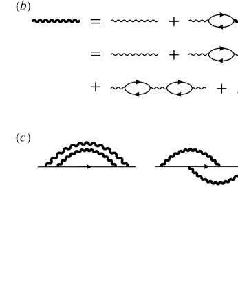
Figure 1: (a) The self-energy diagram relevant in the high-density limit with the thick wiggly line being the dynamically screened Coulomb interaction and the thin wiggly line the bare Coulomb interaction. The solid lines correspond to the electron Green functions; (b) The dynamically screened Coulomb interaction infinite series in the bare interaction through the bubble diagrams. A bubble corresponds to the noninteracting (“Lindhard”) polarizability. (c) Examples of higher order diagrams which are negligible in the high density limit but are important at lower densities.

Within leading order perturbation theory, one can use the bare electron Green function in Eq. (II.2), which can be written as

$$G_{R}^{(0)}\left(\varepsilon,{\bf p}\right)=\left[\varepsilon-\xi^{(0)}_{\bf p}+i0\right]^{-1}.$$

If the effective interaction is isotropic (which indeed is the case in the jellium model we wish to study), the integral(s) over the directions of ${\bf q}$ can be evaluated and we obtain the following expressions for the real part of the retarded self-energy function:

$$\operatorname{Re}\Sigma_{R}\left(\varepsilon,\xi_{\bf p}\right)=\Sigma_{1}\left(\varepsilon,\xi_{p}\right)+\Sigma_{2}\left(\varepsilon,\xi_{p}\right),$$ (11)

where in three dimensions:

$$\Sigma_{1}^{(3D)}\left(\varepsilon,\xi_{p}\right)=\frac{1}{8\pi^{2}v_{\rm F}}\fint\limits_{-\infty}^{+\infty}d\omega\int\limits_{q_{1}(\Omega)}^{q_{2}(\Omega)}\!\!\!dqq\operatorname{Re}D_{R}\left(\omega,q\right)\tanh\left[\frac{\omega+\varepsilon}{2T}\right]$$ (12)

and

$$\Sigma_{2}^{(3D)}\left(\varepsilon,\xi_{p}\right)= \!\!\!\!\!\!-\frac{1}{8\pi^{3}v_{\rm F}}\fint\limits_{-\infty}^{+\infty}d\omega\int\limits_{0}^{\infty}dqq\ln\left|\frac{\Omega-q^{2}/{2m}+v_{\rm F}q}{\Omega-q^{2}/{2m}-v_{\rm F}q}\right|$$ (13)

$$\!\!\!\!\!\!\times\operatorname{Im}D_{R}\left(\omega,q\right)\coth\left[\frac{\omega}{2T}\right],$$

and in two dimensions

$$\Sigma_{1}^{(2D)}\left(\varepsilon,\xi_{p}\right)= \!\!\!\!\frac{1}{4\pi^{2}v_{\rm F}}\fint\limits_{-\infty}^{+\infty}d\omega\int\limits_{q_{1}(\Omega)}^{q_{2}(\Omega)}\frac{dq}{\sqrt{1-\left(\frac{\Omega-q^{2}/{2m}}{v_{\rm F}q}\right)^{2}}}$$ (14)

$$\!\!\!\!\times\operatorname{Re}D_{R}\left(\omega,q\right)\tanh\left[\frac{\omega+\varepsilon}{2T}\right]$$

and

$$\Sigma_{2}^{(2D)}\left(\varepsilon,\xi_{p}\right)=-\frac{1}{4\pi^{2}v_{\rm F}}\fint\limits_{-\infty}^{+\infty}d\omega\left[\int\limits_{0}^{q_{1}(\Omega)}+\int\limits_{q_{2}(\Omega)}^{\infty}\right]$$

$$\times\frac{dq}{\sqrt{\left(\frac{\Omega-q^{2}/{2m}}{v_{\rm F}q}\right)^{2}-1}}\operatorname{Im}D_{R}\left(\omega,q\right)\coth\left[\frac{\omega}{2T}\right].$$ (15)

In Eqs. (12), (13), (14), and (II.2), we introduced the following notations for the sake of brevity:

$$\Omega=\omega+\varepsilon-\xi_{p}$$

and $q_{2}\left(\Omega\right)\geq q_{1}\left(\Omega\right)\geq 0$ which are the solutions of the equation $\left|\Omega-q^{2}/{2m}\right|=v_{\rm F}q$.

II.3 Effective interaction and the polarization operator.

The appropriate propagator in the case of an electron liquid with long-range Coulombic forces between electrons is given by the sum of the ladder of bubble diagrams and has the typical RPA form (see Fig. 1b):

$$D(\omega,q)={V(q)\over 1+V(q)\Pi(\omega,q)},$$ (16)

where $V(q)$ is the bare Coulomb interaction [$V(q)=4\pi e^{2}/q^{2}$ in three dimensions and $V(q)=2\pi e^{2}/q$ in two dimensions] and $\Pi(\omega,q)$ is the polarizability bubble:

$$\Pi\left(\omega,{\bf q}\right)=2\int{d\varepsilon\,d^{d}{\bf p}\over\left(2\pi\right)^{(1+d)}}G^{(0)}\left(\varepsilon,{\bf p}\right)G^{(0)}\left({\varepsilon+\omega},{\bf p+q}\right).$$ (17)

At zero temperature, the polarizability was calculated by LindhardLindhard (1954) and SternStern (1967) in three and two dimensions respectively. We will need the exact expressions, which can be conveniently written in terms of the dimensionless parameters $u=\omega/\left(v_{\rm F}q\right)$ and $x=q/(2p_{\rm F})$. In three dimensions it reads

$$\operatorname{Re}\Pi^{(3D)}\left(u,x\right)=\frac{\nu^{(3D)}}{2}\Biggl{\{} \!\!\!\!\!\!1+{1\over 4x}\left[1-\left(x+u\right)^{2}\right]\ln\left|\frac{1+x+u}{1-x-u}\right|$$ (18)

$$\!\!\!\!\!\!\!\!\!\!\!+{1\over 4x}\left[1-\left(x-u\right)^{2}\right]\ln\left|\frac{1+x-u}{1-x+u}\right|\Biggr{\}}$$

and the imaginary part for $u>0$ [$\operatorname{Im}\Pi\left(u,x\right)=-\operatorname{Im}\Pi\left(-u,x\right)$]:

$$\operatorname{Im}\Pi^{(3D)}\left(u,x\right)=-\frac{\pi\nu^{(3D)}}{2}\Biggl{\{}u\,\,\theta\left(\left|1-x\right|-u\right)$$

$$+\frac{1}{x}\left[1-\left(x-u\right)^{2}\right]\theta\left(\left|1+x\right|-u\right)\theta\left(u-\left|1-x\right|\right)\Biggr{\}},$$ (19)

where $\nu^{(3D)}=mp/\pi^{2}$ is the density of states at the Fermi surface.

In two dimensions the polarizability has the following explicit form:

$$\operatorname{Re}\Pi^{(2D)}\left(u,x\right)=\nu^{(2D)}\operatorname{Re}\Biggl{\{}1-{{\rm sgn\,}\left(x+u\right)\over 2x}\sqrt{\left(x+u\right)^{2}-1}$$

$$\!\!\!\!-{{\rm sgn\,}\left(x-u\right)\over 2x}\sqrt{\left(x-u\right)^{2}-1}\Biggr{\}}$$ (20)

and the imaginary part for any $u$:

$$\!\!\operatorname{Im}\Pi^{(2D)}\!\left(u,x\right)=\!\!\frac{\nu^{(2D)}}{2x}\operatorname{Re}\Biggl{\{}\!\!\!\sqrt{1-\left(x+u\right)^{2}}-\!\!\sqrt{1-\left(x-u\right)^{2}}\Biggr{\}},$$ (21)

with $\nu^{(2D)}=m/\pi$ being the two-dimensional density of states at the Fermi line.

Let us emphasize that both three dimensional and two dimensional polarizabilities are non-analytic functions at $\left|u\pm x\right|=1$. Usually this singularity is associated with Friedel oscillations and Kohn-Luttinger effect,Kohn and Luttinger (1965) i.e. with the famous Kohn anomaly at $q=2p_{\rm F}$ and $\omega\to 0$. In the case of a dense Coulomb liquid, the typical momenta are small $x=q/(2p_{\rm F})\ll 1$, but $u=\omega/(v_{\rm F}q)$ can be of the order of unity or even larger. As we shall see, exactly this domain of parameters (i.e., small momentum transfers) is responsible for non-analytic contributions to the effective mass temperature dependence and the quasiparticle $Z$-factor. The usual Kohn singularity ($x=1$) in the static polarizability also gives rise to a non-analytic temperature dependence but this effect is parametrically smaller than the dynamic screening effects in the limit $r_{\rm s}\ll 1$.

The issue of the temperature dependence of the polarization operator was recently reconsidered in great details by Chubukov and MaslovChubukov and Maslov (2003) (see also Refs. [Stern, 1980] and [Das Sarma, 1986]) who found that in the vicinity of the Kohn singularity the polarizability has a linear $T$ correction, which is important in the case of a short range interaction case. In the case of the long-range Coulombic forces, the $q$-dependence of the propagator (16) becomes crucial and in the high-density limit the results are determined by the region $x=q/(2p_{\rm F})\sim r_{\rm s}\ll 1$ in two dimensions ($x\sim\sqrt{r_{\rm s}}$ in three dimensions). Hence, in the leading order in $r_{\rm s}$, only the region $x\ll 1$ is important. In this region, the leading temperature correction to the polarizability is of the order of $T^{2}$ in any dimensionality. As we shall see below, the leading order temperature corrections to the effective mass and the $Z$-factor are parametrically larger than $T^{2}$. Therefore, in the high-density limit, the temperature corrections to the polarization bubble give negligible contributions to the quasiparticle spectrum and in the case $T/E_{\rm F}\ll r_{\rm s}\ll 1$, one can use the zero temperature results for the polarizability [see Eqs. (18), (II.3), (II.3), and (21)] in the calculations of the effective mass and the $Z$-factor.

II.4 Collective modes

The usual practice is to expand the polarizability functions in $x\ll 1$; in which case the polarizability becomes the function of just one variable $u=\omega/(v_{\rm F}q)$. The limit $u\ll 1$ corresponds to the electron-hole branch of excitations. The corresponding retarded electron-hole propagator is (in three dimensions)

$$D_{\rm eh}^{(3D)}(\omega,q)=4\pi e^{2}\left[q^{2}+\varkappa_{3}^{2}-i{\pi\over 2}\varkappa_{3}^{2}\left({\omega\over v_{\rm F}q}\right)\right]^{-1},$$ (22)

where $\varkappa_{3}=2p_{F}\sqrt{\alpha^{(2D)}}$ is the inverse screening length.

In two dimensions the electron-hole propagator reads

$$D_{\rm eh}^{(2D)}(\omega,q)=2\pi e^{2}\left[q+\varkappa_{2}-i\varkappa_{2}\left({\omega\over v_{\rm F}q}\right)\right]^{-1},$$ (23)

where $\varkappa_{2}=2p_{F}\alpha^{(2D)}$ is the inverse screening length in two dimensions.

The opposite limit $u\gg 1$ corresponds to the plasmon branch. The spectrum of plasma waves is determined by the equation

$$1+V(q)\Pi(\omega,q)=0.$$

In three dimensions the spectrum has the following well-known form $\omega_{\rm pl}^{(3D)}(q)=\sqrt{\omega_{0}^{2}+{3\over 5}v_{\rm F}^{2}q^{2}}$, with $\omega_{0}=4\pi e^{2}n/m$. In two dimensions, the plasmons are gapless $\omega_{\rm pl}^{(2D)}(q)=\sqrt{aq+bq^{2}}$ with $a=2e^{2}E_{\rm F}$ and $b={3E_{\rm F}/(2m)}$.

Within the first approximation in the interaction, the imaginary part of the polarization operator at $\omega\gg v_{\rm F}q$ is zero. This is exactly the source of the well-known plasmon singularity in self-energy calculations. However, higher order diagrams deliver non-zero contributions to the imaginary part. Taking into account this fact, we can write down the following expression for the retarded plasmon propagator:

$$D_{\rm pl}(\omega,q)={1\over 2}V(q)\omega\Big{[} \!\!\!\!\!{1\over\omega-\omega_{\rm pl}(q)+i0}$$ (24)

$$\!\!\!\!\!+{1\over\omega+\omega_{\rm pl}(q)+i0}\Big{]}\theta\left(q_{\rm m}-q\right),$$

where $q_{\rm m}$ is the wave-vector at which the strong Landau damping commences.

We shall see that the leading temperature correction to the effective mass both in two and three dimensions comes mostly from the region of $u\sim 1$, which is neither plasmon nor electron-hole region. In actual calculations, we do not separate the screened Coulomb propagator into the electron-hole and plasmon branches. Moreover, for the calculation of the renormalization factor one is required to keep the exact polarizability function (without expanding on $x\to 0$).

III Three-dimensional case

In this section we present analytic calculations of the effective mass and the quasiparticle $Z$-factor in a three-dimensional dense electron liquid. Throughout this section, $\nu=mp/\pi^{2}$ is the three-dimensional density of states and $\alpha=e^{2}/\left(\pi\hbar v_{\rm F}\right)$ is the appropriate expansion parameter. The main results are Eqs. (29) and (34) given below.

III.1 Effective mass

In the high density limit, the correction to the effective mass is determined by the on-shell equation (8), which means that we can put $\varepsilon=\xi_{p}$ and study the self-energy as a function of just one variable [see Eqs. (18)]. On the shell, we have the following expression:

$${\partial\over\partial\xi}\operatorname{Re}\Sigma\left(\epsilon=\xi,\xi\right)\Biggr{|}_{\xi=0}= \frac{1}{8\pi^{2}v_{\rm F}}\fint\limits_{-\infty}^{+\infty}{d\omega\over 2T}{1\over\cosh^{2}\left[{\omega\over 2T}\right]}$$ (25)

$$\times\int\limits_{q_{1}[\omega-E_{0}(q)]}^{q_{2}[\omega-E_{0}(q)]}\!\!\!dqq\operatorname{Re}D\left(\omega,q\right).$$

It is convenient to separate the static and dynamic propagators:

$$D(\omega,q)=D_{\rm st}(q)+D_{\rm dyn}(\omega,q)\equiv D(0,q)+\left[D(\omega,q)-D(0,q)\right].$$ (26)

The static propagator has the form:

$$D_{\rm st}(x)={\alpha\over\nu}\,{1\over x^{2}+\alpha}.$$ (27)

At low temperatures, frequencies $\omega$ in the integral (25) are of the order of temperature or even lower. We consider the following asymptotic regime of ultra-low temperatures:

$$\delta=\omega/(4E_{\rm F})\sim T/E_{\rm F}\ll\alpha\ll 1.$$

In this limit, the real part of the dynamic propagator has following form [see Eq. (18), (II.3)]:

$$\operatorname{Re}D_{\rm dyn}(\delta,x)= \!\!\!\!\!\!\!-{\alpha\over\nu}\,\left({\pi\alpha\delta\over 2}\right)^{2}\left(x^{2}+\alpha\right)^{-1}$$ (28)

$$\!\!\!\!\!\!\!\times\left[x^{2}\left(x^{2}+\alpha\right)^{2}+\left({\pi\alpha\delta\over 2}\right)^{2}\right]^{-1}.$$

Using Eq. (25) and propagators (27) and (28), one can calculate corrections to the effective mass (expanding on the small parameter $\delta\sim T/E_{\rm F}$) and see that the static contribution, indeed, solely determines the renormalization of the effective mass at zero temperature. However, it gives temperature corrections of the order of $T^{2}$ only. The dynamic part gives zero contribution to the zero temperature effective mass, but gives parametrically larger temperature dependent correction. The final result reads:

$${m^{*}\left(T\right)-m\over m}=-{\alpha\over 2}\ln{1\over\alpha}+{\pi^{2}\over 96}\left(T\over E_{\rm F}\right)^{2}\ln{E_{\rm F}\over T}.$$ (29)

The first term indeed coincides with the old result of Gell-Mann. The non-analytic temperature correction given in the second term of Eq. (29) is a new result. Let us emphasize that the leading correction is positive only in the high-density limit. In Ref. [Das Sarma et al., ], it was shown that the leading $T^{2}\ln{T}$ correction changes sign at lower densities ($\alpha^{(3D)}\sim 1$). The density dependence comes from large momentum transfers $q$, in particular from the vicinity of the $2p_{\rm F}$-anomaly, which becomes increasingly important at lower densities.

III.2 $Z$-factor

Unlike in the effective mass calculation of the preceding section, the quasiparticle $Z$-factor can not be calculated within the on-shell method, and therefore the problem is more complicated. In particular, one has to consider both contributions to the self-energy given in (12) and (13). The first contribution at zero temperature reads:

$${\partial\over\partial\varepsilon}\Sigma_{1}\left(\varepsilon,\xi=0\right)\Biggr{|}_{\varepsilon=0}={\nu\over 2}\int\limits_{0}^{\infty}dxx\fint\limits_{-\infty}^{\infty}du\operatorname{Re}D\left(u,x\right)$$

$$\times{\partial\over\partial u}\left[\theta\left(1-\left|u-x\right|\right){\rm sgn\,}u\right].$$ (30)

In the three-dimensional case, the integral over $u$ reduces to a $\delta$-function integration and we have:

$${\partial\over\partial\varepsilon}\Sigma_{1}\left(\varepsilon,\xi=0\right)\Biggr{|}_{\varepsilon=0}\!\!\!\!\!\!=\nu\int\limits_{0}^{1}dxx\Biggl{[} \!\!\!\!\!D\left(0,x\right)-{1\over 2}\operatorname{Re}D\left(1+x,x\right)$$ (31)

$$\!\!\!\!\!\!\!\!\!-{1\over 2}\operatorname{Re}D\left(1-x,x\right)\Biggr{]}.$$

From Eq. (13), we derive the second contribution:

$${\partial\over\partial\varepsilon}\Sigma_{2}\left(\varepsilon,\xi=0\right)\Biggr{|}_{\varepsilon=0}\!\!\!\!\!\!= \!\!\!\!\!\!{\nu\over\pi}\int\limits_{0}^{\infty}dx\,x\,\int\limits_{0}^{\infty}\operatorname{Im}D\left(u,x\right)$$ (32)

$$\!\!\!\!\!\!\times\left[{1\over 1-\left(u-x\right)^{2}}+{1\over 1-\left(u+x\right)^{2}}\right].$$

Using Eqs. (18), (II.3), and (24), one can evaluate integrals (31) and (32) and obtain

$${\partial\over\partial\varepsilon}\Sigma\left(\varepsilon,\xi=0\right)\Biggr{|}_{\varepsilon=0}\!\!\!\!\!\!=-{\alpha\over\pi}\int\limits_{0}^{\infty}{du\over 1+u^{2}}\ln\left[{1\over 1-u\,{\rm atan}\,{1\over u}}\right].$$ (33)

Evaluating the remaining integral numerically, we derive the final result for the quasiparticle renormalization factor:

$$Z=1-1.067\alpha.$$ (34)

This asymptotic result is in a very good agreement with numerical simulations.Mahan (1990)

IV Two-dimensional case

In this section we present analytic calculations of the effective mass and quasiparticle $Z$-factor in a two-dimensional dense electron liquid. Throughout this section, $\nu=m/\pi$ is the two dimensional density of states and $\alpha=e^{2}/\left(\hbar v_{\rm F}\right)\ll 1$ is the appropriate expansion parameter. The main results are Eqs. (40), (41), and (46) given below.

IV.1 Effective mass

The calculation of the effective mass in two dimensions is analogous to the calculation in three dimensions (see Sec. III.2). The only difference is the square root function, which appears in all two-dimensional expressions [see, e.g., Eqs. (14) and  (II.2)]. This square root singularity is identical to the singularity in the Stern’s polarizability function given in Eqs. (II.3) and (21). The combination of these two singularities leads to a stronger temperature dependence (linear as we shall see) as compared to the three-dimensional case. From Eqs. (8) and  (14), we get the following on-shell expression for the two-dimensional electron effective mass:

$${m^{*}-m\over m}=-{\nu\over 2\pi}\fint\limits_{-\infty}^{\infty}{d\omega\over 2T}{1\over\cosh^{2}{\omega\over 2T}}I(\omega),$$ (35)

where we have introduced the following integral:

$$I(\omega)=\int\limits_{x_{1}(\omega)}^{x_{2}(\omega)}dx{x\operatorname{Re}D\left(\omega,x\right)\over\sqrt{\left[x^{2}-x_{1}^{2}(\omega)\right]\left[x_{2}^{2}(\omega)-x^{2}\right]}},$$ (36)

where $x=q/\left(2p_{\rm F}\right)$ and $x_{1,2}$ are the solutions of the equation $\left|{\omega\over 4E_{\rm F}x}-x\right|=1$. In the limit of low temperatures: $x_{1}\approx\left|\delta\right|=\left|\omega\right|/(4E_{\rm F})$ and $x_{2}\approx 1$.

Again we re-write the propagator as a sum of static and dynamic terms (26). The two-dimensional static propagator has the form

$$D_{\rm st}(x)={\alpha\over\nu}{1\over x+\alpha}.$$ (37)

The real part of the dynamic propagator in the limit $|\omega|\sim T\ll E_{\rm F}$ reads:

$$\operatorname{Re}D_{\rm dyn}(\delta,x)= \!\!\!\!\!\!\!-{\alpha\over\nu}\,\left(\alpha\operatorname{Im}\Pi\right)^{2}\left(x+\alpha\right)^{-1}$$ (39)

$$\!\!\!\!\!\!\!\times\left[\left(x+\alpha\right)^{2}+\left(\alpha\operatorname{Im}\Pi\right)^{2}\right]^{-1},$$

where $\operatorname{Im}\Pi$ is defined by Eq. (21).

Expanding in the small parameter $\delta$, we obtain the contribution to the integral (36) due to the static propagator

$$I_{\rm st}(\delta)={\alpha\over\nu}\left[\ln{1\over\alpha}-{\delta^{2}\over 2\alpha^{2}}\ln{1\over\left|\delta\right|}\right]$$

and the “dynamic part”

$$I_{\rm dyn}(\delta)={\alpha\over\nu}\left[-{\pi\over 2}{\left|\delta\right|\over\alpha}+{3\delta^{2}\over\alpha^{2}}\ln{1\over\left|\delta\right|}\right].$$

Evaluating the elementary integral, we obtain the final result for the temperature dependent effective mass in the second leading order in temperature:

$${m^{*}\left(T\right)-m\over m}=-{\alpha\over\pi}\ln{1\over\alpha}+{\ln{2}\over 4}\left(T\over E_{\rm F}\right)-{5\pi\over 48\alpha}\left(T\over E_{\rm F}\right)^{2}\ln{E_{\rm F}\over T}.$$ (40)

Let us emphasize that Eq. (40) is valid in the low temperature and high-density limit: $T/E_{\rm F}\ll\alpha\ll 1$ and only for subthermal particles: $\varepsilon\ll T$. We see that the leading term is linear in temperature and the coefficient is a universal density independent number. This universal behavior is true only in the high density limit. There are other linear-$T$ contributions, such as the one due to the temperature dependence of the polarizability in the vicinity of the Kohn singularity (considered in the paper of Chubukov and Maslov Chubukov and Maslov (2003) for short-range interactions). In the case of the long-range Coulomb interaction, the Kohn anomaly leads to a linear-$T$ term proportional to the Coulomb expansion parameter $\alpha$. Similar $\alpha$-dependence of the linear slope was discovered in RPA numerical calculations in Ref. [Das Sarma et al., ]. In the high-density limit, this density dependent linear-$T$ term is asymptotically smaller than the main universal contribution [the second term in Eq. (40)] and therefore not shown in Eq. (40).

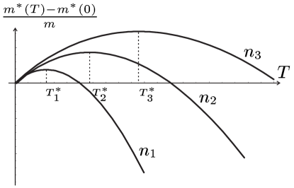
Figure 2: Asymptotic effective mass temperature dependence [see Eq. (40)] for three different densities $n_{1}>n_{2}>n_{3}$. The slope of the curves is universal at high densities [$\sqrt{n}/(me^{2})\gg 1$].

From Eq. (40), we see that the effective mass temperature dependence is non-monotonic. A maximum occurs at a temperature $T^{*}$, which within the logarithmic accuracy has the form:

$${T^{*}\over E_{\rm F}}={6\ln{2}\over 5\pi}\,{\alpha\over\ln{1\over\alpha}}\approx 0.26\,{\alpha\over\ln{1\over\alpha}}\ll\alpha.$$ (41)

This result is formally within the limits of applicability of our theory. We see that the point of maximum of the curve $m^{*}(T)$ drifts toward higher temperatures as the density decreases. This tendency is preserved at lower densities as well (within the RPA approach). Such a maximum in $m^{*}(T)$ and a density dependent $T^{*}$ were also discovered in our recent numerical calculation.Das Sarma et al.

IV.2 $Z$-factor

The analytical calculation of the $Z$-factor in two dimensions is technically a very demanding problem. The mixture of two singularities, the Kohn singularity in the polarizability and the identical square root singularity in Eqs. (14) and (II.2) arising from the two-dimensional phase space, leads to a complicated structure of the integrals in Eqs. (14) and (II.2), each being a truly divergent quantity. The logarithmic divergence gets cancelled (at least within the RPA), but to see this cancellation one is required to keep the exact $x$ and $u$ dependences in the Stern’s polarizability function. Moreover, the technical method used in the three-dimensional calculation of the $Z$-factor [see Sec. III.2, Eq. (III.2)] is not applicable here because of the square-root singularity.

Let us now study the two-dimensional $Z$-factor in more details. The quasiparticle renormalization factor is determined by the energy derivative of the self-energy. The latter can be written as a sum of two terms [see Eqs. (14) and (II.2)]:

$${\partial\over\partial\varepsilon}\Sigma_{1}\left(\varepsilon,\xi=0\right)\Biggr{|}_{\varepsilon\to 0}\!\!\!\!= \!\!\!\!-{\nu\over 2\pi}\int\limits_{0}^{\infty}dxx\int\limits_{0}^{\infty}du\left[{\partial\over\partial u}\operatorname{Re}D\left(u,x\right)\right]$$ (42)

$$\!\!\!\!\!\!\!\!\!\!\!\!\times\left[{\theta\left(1-\left|u-x\right|\right)\over\sqrt{1-\left(u-x\right)^{2}}}+{\theta\left(1-\left|u+x\right|\right)\over\sqrt{1-\left(u+x\right)^{2}}}\right]$$

and

$${\partial\over\partial\varepsilon}\Sigma_{2}\left(\varepsilon,\xi=0\right)\Biggr{|}_{\varepsilon\to 0}={\nu\over 2\pi}\int\limits_{0}^{\infty}dxx\int\limits_{0}^{\infty}du\left[{\partial\over\partial u}\operatorname{Im}D\left(u,x\right)\right]$$

$$\times\left[{\theta\left(\left|u-x\right|-1\right)\over\sqrt{\left(u-x\right)^{2}-1}}-{\theta\left(\left|u+x\right|-1\right)\over\sqrt{\left(u+x\right)^{2}-1}}\right].$$ (43)

The frequency dependence (hence, the $u$-dependence) of the propagator $D(u,x)$ is due to the polarizability $\Pi(u,x)$, which contains exactly the same square root functions as the ones in Eqs. (42) and (IV.2). This leads to a logarithmic divergence of each of the above integrals at $u=1\pm x$. The “singular” contributions have the following forms:

$${\partial\over\partial\varepsilon}\Sigma_{1}^{\rm(sing)}\left(\varepsilon,\xi=0\right)\Biggr{|}_{\varepsilon\to 0}={1\over\pi}\int\limits_{0}^{\infty}dxx\int\limits_{0}^{1+x}du{\left[\operatorname{Re}D\left(u,x\right)\right]^{2}\over\sqrt{1-\left(u-x\right)^{2}}}$$

$$\times{\partial\operatorname{Im}\Pi\over\partial u}\operatorname{Im}\Pi\,\left[x+{\alpha\over\nu}\operatorname{Re}\Pi\right]$$ (44)

and

$${\partial\over\partial\varepsilon}\Sigma_{2}^{\rm(sing)}\left(\varepsilon,\xi=0\right)\Biggr{|}_{\varepsilon\to 0}={1\over\pi}\int\limits_{0}^{\infty}dxx\int\limits_{1-x}^{0}du{\left[\operatorname{Re}D\left(u,x\right)\right]^{2}\over\sqrt{\left(u+x\right)^{2}-1}}$$

$$\times{\partial\operatorname{Re}\Pi\over\partial u}\operatorname{Im}\Pi\,\left[x+{\alpha\over\nu}\operatorname{Re}\Pi\right].$$ (45)

Each of these quantities is logarithmically divergent $\left({\partial\Sigma_{1,2}\over\partial\varepsilon}\right)\sim\pm\alpha\ln{\varepsilon}\to\infty$. We emphasize that in two dimensions the real and imaginary parts of the polarizability have almost identical analytic structures, in contrast to the three dimensional case in which the imaginary and real parts are basically independent functions with quite different properties. Using Eqs. (IV.2) and (IV.2), one can check that this “symmetry” of the two-dimensional polarizability leads to an exact cancellation of the logarithmic divergence and to a finite result.

Let us emphasize that this kind of dangerous singularities appear in any order of the perturbation theory in interaction (see, e.g., Fig. 1c). It is not a priori obvious how (and if) the singularity, which is cut-off only by temperature or energy $\varepsilon$, is cancelled in higher order diagrams. We do not have a general argument for why the divergence must cancel in each order, but we do know that they cancel to this order. It is essential to clarify this point to assure that the quasiparticle $Z$-factor does not vanish logarithmically $Z^{-1}(\varepsilon)\sim\ln{\varepsilon}$ and to make certain that the usual Landau Fermi liquid theory is preserved in two dimensions. This issue is currently being studied by us. We believe that the Fermi liquid theory is preserved but it needs to be demonstrated explicitly.

Within the RPA, the zero temperature $Z$-factor can be proven to be finite.Jalabert and Das Sarma (1989) One can formally define the quasiparticle $Z$-factor at finite temperatures via relation (7). Studying the leading temperature correction to the energy derivative of the self-energy is quite similar to the case of the on-shell derivative case. The leading term can be shown to be linear and negative:Burkard et al. (2000)

$$Z(\alpha,T)\approx 1-\left({1\over 2}+{1\over\pi}\right)\alpha-c\,\left({T\over E_{\rm F}}\right),$$ (46)

where $c$ is a constant of the order of unity.

V Conclusion

In this work we have developed the analytic leading order theory for the temperature dependent quasiparticle effective mass, $m^{*}(T)$, and the quasiparticle renormalization factor for two- and three-dimensional interacting electron systems. Our results are asymptotically exact in the low temperature high-density limits for the case of the realistic long-range Coulomb interaction, and thus we are complementary to the recent analytical work of Ref. [Chubukov and Maslov, 2003], which considers a short-range repulsive interaction. It is interesting to note that $m^{*}(T)$ has an unexpected linear-$T$ correction (rather than $T^{2}$) both in our theory and in the theory of Chubukov and Maslov; but in our case the correction is positive opposite to the short range case. This immediately leads to the conclusion that the leading correction to $C_{V}/T$ (where $C_{V}$ is the specific heat) is not universal — our long range interaction produces a positive linear-$T$ term in the leading order in contrast to the negative sign obtained in Ref. [Chubukov and Maslov, 2003]. This unexpected linear-$T$ term appears due to the non-analyticity of the polarizability function. This non-analyticity has potentially important consequences for quantum critical phenomena as discussed recently in Ref. [Chubukov et al., ].

Our analytic results are also in agreement with recent numerical studies of the temperature dependent effective mass,Das Sarma et al. which employed the random-phase approximation at lower densities. It was shown that the linear-$T$ correction persists at lower densities as well (at least within the RPA) and the qualitative behavior of the effective mass remains the same with the only difference being the density dependent slope of the $m^{*}(T)$ curve at $T\to 0$ and $r_{\rm s}>1$ (for high densities, it was shown to be density independent in agreement with the analytical results reported in the present paper). As the RPA is believed to be qualitatively reliable at lower densities as well, we expect our results to be quite general and qualitatively applicable to realistic two-dimensional electron systems. We also should point out that although the temperature dependent effective mass renormalization has only been calculated numerically very recently,Das Sarma et al. there is a vast literature of numerical studies of zero temperature many-body effects in the three-dimensional and two-dimensional interacting electron systems. We cite in this context only two rather comprehensive references: Ref. [Hedin and Lundqvist, ] for three-dimensional systems and Ref. [Jalabert and Das Sarma, 1989] for two-dimensional systems.

We have proved that the quasiparticle $Z$-factor in two dimensions is finite at least within the random-phase approximation. However, we would like to emphasize that each order in perturbation theory does contain a dangerous logarithmic singularity in this quantity. It is known that in two dimensions higher order diagrams may contain important effects (see, e.g., Ref. [Chubukov, 1993], in which it was shown that the static Kohn-Luttinger effectKohn and Luttinger (1965) in two dimensions is “hidden” in third order perturbation theory only). It is therefore essential to prove that the cancellation of the logarithmic singularity (which would otherwise lead to a logarithmically vanishing $Z$-factor and to a marginal Fermi liquidLittlewood and Varma (1992)) takes place in higher orders. This important question will be considered elsewhere.

- (1) A. V. Chubukov and D. L. Maslov, eprint cond-mat/0304381.
- Chubukov and Maslov (2003) A. V. Chubukov and D. L. Maslov, Phys. Rev. B 68, 155113 (2003).
- (3) S. Das Sarma, V. M. Galitski, and Y. Zhang, eprint cond-mat/03033632.
- Gell-Mann (1957) M. Gell-Mann, Phys. Rev. B 106, 369 (1957).
- Galitskii (1958) V. M. Galitskii, Sov. Phys. - JETP 7, 104 (1958).
- Chaplik (1971) A. V. Chaplik, Sov. Phys. - JETP 33, 997 (1971).
- Giuliani and Quinn (1982) G. F. Giuliani and J. J. Quinn, Phys. Rev. B 26, 4421 (1982).
- Abrikosov et al. (1963) A. A. Abrikosov, L. P. Gor’kov, and I. E. Dzyaloshinski, Methods of quantum field theory in statistical physics (Dover Publications, New York, 1963).
- Mahan (1990) G. D. Mahan, Many-Particle Physics (Plenum Press, New York and London, 1990).
- Lindhard (1954) J. Lindhard, K. Dan. Vidensk. Selsk. Mat. Fys. Medd. 28, 8 (1954).
- Stern (1967) F. Stern, Phys. Rev. Lett. 18, 546 (1967).
- Kohn and Luttinger (1965) W. Kohn and J. H. Luttinger, Phys. Rev. Lett. 15, 524 (1965).
- Stern (1980) F. Stern, Phys. Rev. Lett. 44, 1469 (1980).
- Das Sarma (1986) S. Das Sarma, Phys. Rev. B 33, 5401 (1986).
- Jalabert and Das Sarma (1989) R. Jalabert and S. Das Sarma, Phys. Rev. B 40, 9723 (1989).
- Burkard et al. (2000) G. Burkard, D. Loss, and E. V. Sukhorukov, Phys. Rev. B 61 (2000).
- (17) A. V. Chubukov, C. Pépin, and J. Rech, eprint cond-mat/0311420.
- (18) L. Hedin and S. Lundqvist, in Solid State Physics, edited by H. Ehrenreich, F. Seitz, and D. Turnbull (Academic, New York, 1969), Vol. 23, p. 135; L. Hedin, Phys. Rev. 139, A796 (1965).
- Chubukov (1993) A. V. Chubukov, Phys. Rev. B 48, 1097 (1993).
- Littlewood and Varma (1992) P. B. Littlewood and C. M. Varma, Phys. Rev. B 46, 405 (1992).